Water Resources Evaluation and Sustainability Considering Climate Change and Future Anthropic Demands in the Arequipa Region of Southern Peru

Abstract

Climate change and increases in human activities are threatening water availability in the Arequipa Region (southern Peru). However, to date, there has not been a comprehensive inventory of surface water data or an investigation of current surface water conditions or forecasted future conditions resulting from increased anthropic demand or stresses from climate change. This study evaluates surface water resources management including storage, diversions, and conveyance in the Arequipa Region, while creating a tool for the evaluation of future scenarios in the five main watersheds of this arid region of southern Peru. State-of-the art, open-source modeling software was used. Water uses for each watershed were evaluated against predicted reservoir inflows and streamflows for different periods. In addition to the above, 12 climate change models and different shared socioeconomic pathways (SSP) were ensembled for the five watersheds. A semi-distributed approach and an innovative simulation splitting approach was used for each watershed, which allowed for different starting dates for the simulations using all available data obtained from different sources (government and private). Results indicate that the region is expected to have increased flows during the wet season and no significant changes during the dry season. Reservoir inflows are expected to increase up to 42 and 216% for the lowest and highest SSP evaluated, respectively. Similarly, the model projected streamflow increases up to 295 and 704%, respectively. Regarding yearly water availability and considering current and future demands for the watersheds under study, water deficits are not expected in the future if current reservoir storage can be maintained, though it is expected that reservoirs won’t be able to store predicted higher flows, so important volumes of water could be lost during the wet season to the ocean by natural drainage. Given the uncertainty of climate change projections, if future water sustainability is desired, storage and irrigation efficiencies should be improved and reservoir sedimentation should be evaluated.

1. Introduction

Peru is a country highly threatened by climate change as a result of its geography, inequalities, and natural resource-dependent economy [1,2], with the main effects being floods, droughts, landslides, and glacial melting; the severity of these effects is expected to be amplified by El Niño Southern Oscillation (ENSO) [3,4]. Studies have been focused on different Peruvian watersheds to evaluate what would be the possible local effects of global warming. However, there is not a single answer for climate change effects on the entire Peruvian territory since results vary by location, final objective, and climate change models being used. For example, the Santa, Mantaro, and Rimac rivers were assessed and a reduction in peak flows was calculated for those three important Peruvian rivers [5]. Moreover, some rivers in the Amazonian regions of Peru are expected to increase their streamflow [6], while the Lake Titicaca basin will have more intense, frequent, and prolonged droughts [7]. However, the complex human development dynamics make it harder to predict future water availability under unpredictable climatic changes [8]. While climate change analysis is usually focused on evaluating precipitation and temperature trends (e.g., [9]), authors around the world are now including human activities when predicting water resources availability (e.g., [10,11,12]).

Considering the above, no significant research has been performed in terms of water resources sustainability involving both climate change and human activities in the Arequipa Region of southern Peru (the focus of this study), besides a few studies in which hydrological models were applied, but without a focus on future climate and water demands. Mendoza et al. [13], for example, used a Soil and Water Assessment Tool (SWAT) model in the Tambo watershed (excluding the drainage area for Pasto Grande, the watershed’s main reservoir), while Coloma [14] applied a combination of hydrologic and hydraulic modeling, focusing on the lowest stream gage in that same watershed, using Hydrologic Engineering Center-Hydrologic Modeling System (HEC-HMS) and HEC’s River Analysis System (HEC-RAS) models to analyze return periods. Similarly, the United States Agency for International Development (USAID) [15] applied a Water Evaluation and Planning System (WEAP) model to the Quilca watershed, including most of the individual water uses and “naturalizing” all of the reservoirs in the area. Also, in the Quilca watershed, Wei et al. [16] developed a SWAT model to assess the connection between intensive irrigation and groundwater return flows to an adjacent river in the Majes district, concluding that most of the applied irrigated water is lost through percolation, while Daneshvar et al. [17] applied a SWAT model in the El Frayle reservoir (Quilca watershed) using the streamflow naturalization approach. However, while water consumption in the Arequipa Region continues to increase, the combined effects of both climate change and human activities on water resources availability is currently unknown. Furthermore, water governance in the Region is deficient and not well known, and while several government and private entities collect hydrological information, such information is spaced and hard to analyze, while the diversions, storage, and transportation of water in the Region are unclear, resulting in a weakness for sustainable water management.

This study was designed to (1) characterize for the first time the future flows and reservoir operations in the five main watersheds of the Arequipa Region; and (2) evaluate surface water resources sustainability in the Region considering both climate change and human activities. Our study differs from what has been carried out before in the Region since it starts with a detailed description of how surface water is managed in each watershed (with the purpose of building the appropriate models), followed by accurate watershed delineation based on available data, model setup and calibration, and ending with climate change scenarios for multiple models and SSPs, in addition to water consumption projections for each study site, all to evaluate sustainability of surface water resources. The analysis was performed for each of the five watersheds and it evaluates changes based on all of the observed available data, and future climate and use projections for each drainage area. Furthermore, yearly water availability and water deficits were evaluated. Special, atypical emphasis was placed on the reservoir network as it regulates the Region’s flows throughout the year. Finally, considering the novelty of this investigation, this manuscript was written in more detail than the average modeling publication, with the intention of having it as a guide for other Peruvian scientists and organizations to replicate the analysis in other watersheds within the country.

2. Study Area and Methods

The extension of the watersheds of interest and the political boundaries of the Arequipa Region are illustrated in Figure 1, all beginning in the Andes Mountains and draining into the Pacific Ocean to the southwest. Geographic, climatic, and population characteristics for each watershed are listed in

Table 1. Selected geographic, climatic, and population characteristics for each watershed under study (Source: [19,20,21,22,23,24,25,26,27,28]).

Watershed	Area (km2)	River Length (Km)	Annual Precipitation (mm)	T Max (°C)	T Min (°C)	Relative Humidity (%)	Wind Speed (m/s)	Simulated Reservoirs	Simulated Water Diversions	Population
Tambo	13,022	297	335.35	18.2	0.4	59.5	2.2	1	1	81,291
Quilca	13,530	275	315.5	27.6	−7.3	59.8	3.3	4	0	1,149,002
Camana	17,049	413	360.9	27.5	−6.9	60.1	9.5	4	2	170,998
Ocoña	15,998	283	397	25	−3.3	60	3.5	0	0	58,387
Yauca	4312	183	350	19	5	60.3	3.7	0	0	27,530

. The climate in those watersheds varies with altitude, with annual precipitation ranging from 0 mm near the coast to 800 mm in the high Andes. The wet season is concentrated during summer months (December through March) [18]. Figure 1 also shows the location of climatic and fluviometric stations, reservoirs, infrastructure flow gages, and water diversions that were used to build the hydrological models. Different activities are carried out for the socioeconomic development of the population that live in those watersheds, allowing the generation of income through agriculture, fishery, commerce, mining, and tourism.

Due to the nature and complexity of this study, the methods described include the hydrological analysis of the five main watersheds within the Arequipa Region of southern Peru, though small portions of other administrative Departments (Moquegua, Puno, Cusco, Apurimac, and Ayacucho) were also considered since they were included within the watersheds’ limits (see Figure 1). All of the tools applied were open source, which allows further collaboration and replicability among any interested party [29]; important since an analysis such as this has never been performed in Peru and it is highly needed in many regions of the country.

Based on available information and communications with local government and private water management entities, each watershed was characterized in terms of where and when water was diverted, stored, and transported (within and between watersheds), all to ensure proper model development. The chosen model was Precipitation-Runoff Modeling System (PRMS), developed by the United States Geological Survey (USGS) (see details in [30]). PRMS was selected since: (1) it has an open source code, making the analysis easier to be replicated in Peru; (2) it is continuously being updated; (3) It has a variety of modules for computing different variables and distributing precipitation and temperatures; (4) it allows the activation/deactivation of Hydrologic Response Units (HRU) of the simulations; (5) it can be easily scripted, which improves its customization; (6) it can simulate all kinds of model complexity; and (7) it can be easily integrated with more advanced codes such as the US Geological Survey modular finite-difference flow model (MODFLOW).

Finally, to facilitate an easy replication of this study in other areas of Peru, a complete and detailed explanation of the procedures used to develop the hydrological models is found in Supplemental Information (SI) 1.

3. Results and Discussion

Considering the nature of this investigation, results and their discussion are displayed combining both water management characteristics and hydrological modeling. A discussion of important results is included in each Section, for clarity and better comprehension of the reader. Additionally, even though some paragraphs herein might correspond to Methods, they were included in this Section since they were a result from the investigation (procedures applied after performing literature review, data gathering, and surface water management characterization).

3.1. Data Gathering and Management

After a remarkable effort, obtained hydroclimatological information needed to run the models was gathered from government and private organizations and organized in a hydroshare folder [31], to make it available to the general public. For hydraulic infrastructure, the main datasets collected were reservoir volumes, precipitation, minimum and maximum temperature, and evaporation rates. Reservoirs were considered in three out of five watersheds (three reservoirs in the Camana, five in the Quilca, and one in the Tambo watersheds). For the Quilca watershed, the Uzuña reservoir was not included for three main reasons: (1) the storage volume is negligible; (2) it was built in the year 2015; and (3) it is disconnected from the main water supply and hydroelectric energy generation systems. Similarly, diversions were considered in two out of five watersheds, with two main diversions in the Camana and Quilca watersheds; both of them start in the Camana watershed, meaning that there is a big dependence of the Quilca watershed on Camana. The first diversion allows water to come from two upstream reservoirs (Pañe and Bamputañe reservoirs) to the top of the Quilca watershed, while the second one was built for diverting flows from the middle of the Camana basin to Quilca; its function is to supply water for the Majes irrigation district, which is located at the edge of the Camana and Quilca watersheds. Details about the reservoirs can be found in

Table 2. Construction year and storage for the reservoirs considered in the Tambo, Quilca, and Camana watersheds [32,33].

Reservoir	Watershed	Year of Construction	Effective Storage (Hm3)	Dead Storage (Hm3)
Pasto Grande	Tambo	1998	161.28	38.72
El Pañe	Camana	1962–1964	99.60	41.3
Bamputañe	Camana	2009	40	1.12
Dique los Españoles	Camana	1992	9.09	2.84
Condoroma	Camana	1981–1985	259	16
Pillones	Quilca	2006	78.50	3.24
Challhuanca	Quilca	2010	25	0.4
El Frayle	Quilca	1956–1958	127.24	8.0
Aguada Blanca	Quilca	1968–1972	30.43	5.32

and a plane view of all of the data gathered is illustrated in Figure 1 (Section 2).

The datasets were available starting from the year 1981, but the simulations had different periods based on available stream and reservoir data. All of them had an ending date of 31 December 2016. The Yauca and Ocoña watersheds did not change their starting periods since they only contain streams. The Camana and Quilca watersheds, however, started as soon as 1 January 2006, which is the first date available in the datasets provided by Arequipa’s Electricity Generating Enterprise (EGASA). Priority was given to the EGASA (private) datasets instead of the Majes Autonomus Authority (AUTODEMA, government) ones, since the latter had incomplete records, which included missing values, different measurements, and missing variables such as spillways for some reservoirs.

Reservoir Characterization

Since the study area is hydrologically unknown, it is important to explain some important details for each reservoir:

-

There is only one reservoir (Pasto Grande) in the Tambo watershed, which has two outlets. The first outlet is a channel that diverts the water to the Moquegua watershed, which is located outside of the basins of interest. The second outlet diverts the water to the Tambo watershed, which receives the spillway flows and an annual volume of 8.2 Hm³ between September and December [33].

-

There are four reservoirs in the Camana watershed, with three of them regulating water supply for the upper Quilca watershed through the “Pañe-Colca” channel, while one regulates water to be diverted downstream to the middle Quilca watershed for irrigation purposes (Majes Irrigation District).

○

The Pañe reservoir has natural inflows and two regulated outflows. The first outflow drifts the water toward the “Pañe-Colca” channel, while the second one diverts the spillway to the Camana watershed through the natural stream network.

○

The Bamputañe reservoir has natural inflows and contributes all its flows to the “Pañe-Colca” channel.

○

The Dique reservoir has three main inflows: (1) the first one is through the “Pañe-Colca” channel, which brings the water from the Pañe and Bamputañe outflows; (2) the second one corresponds to a water intake in the “Antasalla” channel, and (3) the third one has natural inflows coming from the upstream rivers of the Camana watershed. Moreover, it has two outlets, one that diverts the water to the “Zamacola” channel (continuation of the “Pañe-Colca” channel that diverts the water towards the Quilca watershed), and one that routes the spillways to the Camana watershed through what would be the natural routing without infrastructure.

○

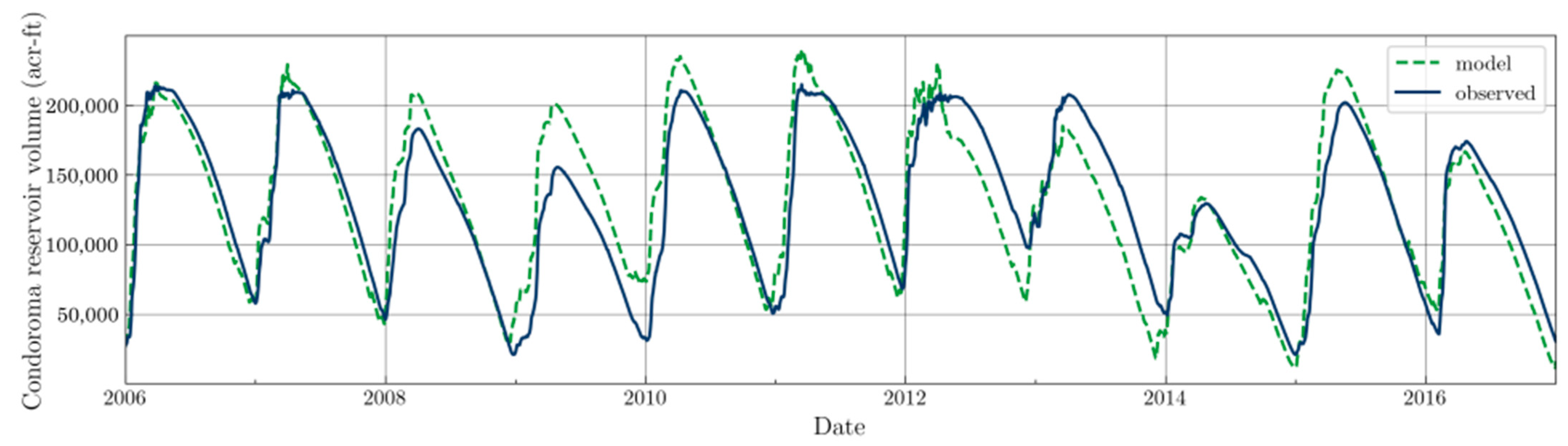
The Condorma reservoir is the biggest reservoir concerning storage in the Camana watershed. It has a natural inflow which is the contribution of its natural drainage area, the spillways from the Pañe reservoir, and the spillways of the Dique reservoir. There is only one outflow for scheduled releases and spillways, and routes the outflow for where it would be the natural routing without infrastructure.

-

For the Quilca watershed, there are also four reservoirs, which have a similar distribution compared to the Camana watershed; three reservoirs are located upstream, while the one downstream gathers the flows of the other three.

○

The Challhuanca reservoir has one natural inflow and only one outflow from where spillway and regulated flows are routed.

○

The Pillones reservoir has two inflows and one outflow. The outflow is through its dam and the inflows come from a tunnel diversion that benefits from the flows coming through the “Zamacola” channel and natural drainage from its basin and the Sumbay one.

○

The “El Frayle” reservoir is similar to the Challhuanca setup, but with a bigger drainage area.

○

The “Aguada Blanca” reservoir receives the outflows from its drainage area, the residual flows left downstream of the Pillones tunnel, and the three aforementioned reservoirs. Regarding its outflows, it has one for regulated outflow and spillway through its dam, and one inner tunnel that diverts flows to a hydroelectric plant (Charcani V), which is located not so far downstream of it.

○

Regarding the Quilca watershed, there is a diversion not so far downstream where the “Zamacola” channel diverts into the Quilca basin, which diverts water into the “Pillones” reservoir. The problem with this diversion is that the remaining downstream flows are not measured and, as a result, the “Aguada Blanca” reservoir calibration will be affected since there is an unmeasured regulated flow (see Figure 2).

For model buildup, the most complicated setup for the reservoirs was the one that connects the “El Pañe”, “Bamputañe”, “Dique los Españoles”, and “Pillones” reservoirs (Camana and Quilca watersheds), mainly due to the fact that there are channels in-between and different inflows and outflows from them. Figure 2 shows a detailed distribution and flow directions for these reservoirs, not only highlighting where data inflows and outflows are located, but also the ones without records. There are many not-mentioned unregulated diversions throughout the extension of the “Pañe-Colca” channel that affected the inflow modeling for the Condoroma reservoir. The same happens for the “Dique los Españoles” reservoir, which has inflows coming from the “Antasalla” and the “Pañe-Colca” channels. In the case of the “Antasalla” channel, all of the inflows coming through this channel and the remaining flows of its upstream river are unknown, which affects the mass balance for the “Dique los Españoles” reservoir and the inflows going into the “Condoroma” reservoir. Regarding the “Pañe-Colca” channel diversion into the “Dique los Españoles” reservoir, there is water being derived into the reservoir by the “Jancolacaya” water intake, which only measures the flows continuing through the channel and not what is going into the reservoir. Luckily, this problem can be taken as a local problem for the “Dique los Españoles” reservoir since flows are measured downstream of the “Pañe-Colca” channel when it changes its name to “Zamacola” channel, which is the channel that takes the water into the Quilca watershed. The effect of all of these unknowns in the inflow volumes for the “Condoroma” reservoir could be negligible since it has the highest storage capacity from its watershed.

3.2. Hydrologic Modeling

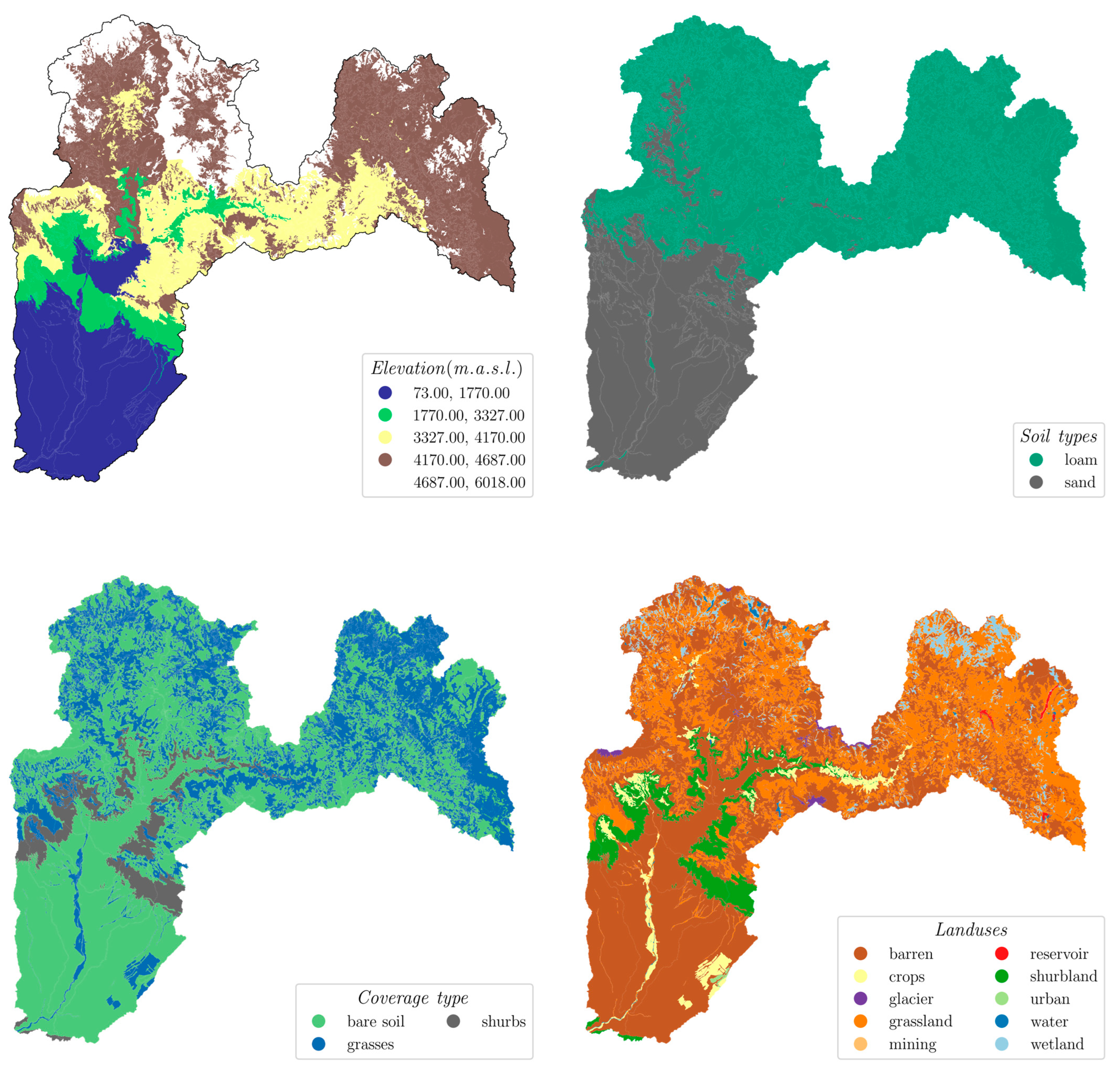
3.2.1. Watershed Delineation and Land Use and Soil Classification

The watershed and land-use delineation required processing of data, so this task is presented in Results, rather than in Methods. The main variables required for the model were elevation, soil type, coverage type, and land use for each HRU, which were defined from the land use data geometries. Soil type was not considered for delineating the HRUs since the datasets found had numerous uncertainties and there were no related comprehensive studies. An example of the distribution of some input variables for simulating one of the watersheds is illustrated in Figure 3.

The delineation of basins and subbasins considered drainage points, where stream gages, diversions, or reservoirs were present. Most of the watersheds had missing areas in the lowest parts of the basins since there are no gages in those places except for the Camana and Ocoña watersheds, which have main cities surrounded by agriculture in those areas. There were at least nine subbasins in each watershed (Figure 4), where the basins with “Cuenca” or “basin” as a prefix in the legend are subbasins found in the National Water Authority (ANA) repositories.

It is important to mention that the way the Quilca watershed was modeled included two drainage points since downstream sub-basins without stream gage data available were not considered in the simulation, being the Pitay watershed the smallest (green-colored watershed in Figure 4). Moreover, the number of HRUs varied among watersheds and the amount has a direct relationship with the running time of each simulation, where Camana required longest run time (see

Table 3. Number of subbasins, HRUs, percentage of area covered by the delineation compared with ANA delineations, and areas for the five watersheds.

	Yauca	Ocoña	Camana	Quilca	Tambo
ANA area (km2)	4.32 × 103	1.60 × 104	1.73 × 104	1.35 × 104	1.30 × 104
Percentage of the area covered by the delineation (%)	94	99	99	77	98
N° HRUs	58	80	5315	2703	70
N° Subbasins	9	11	15	19	12

).

3.2.2. Model Set-Up

For all five watersheds, simulations were performed based on available data (model file descriptions are provided in SI 2, which includes instructions for model files). For the case of watersheds with reservoirs, a multi-basin approach was performed, while for watersheds without them, only one simulation was needed. The number of subbasins per simulation varied from one (when there was just a stream gage) to multiple subbasins. In the case of reservoirs, there were at least two subbasins, from which one corresponded to the reservoir geometry by itself. This approach has the advantage of reduced running times during calibration, as HRUs of subbasins can be inactivated if needed.

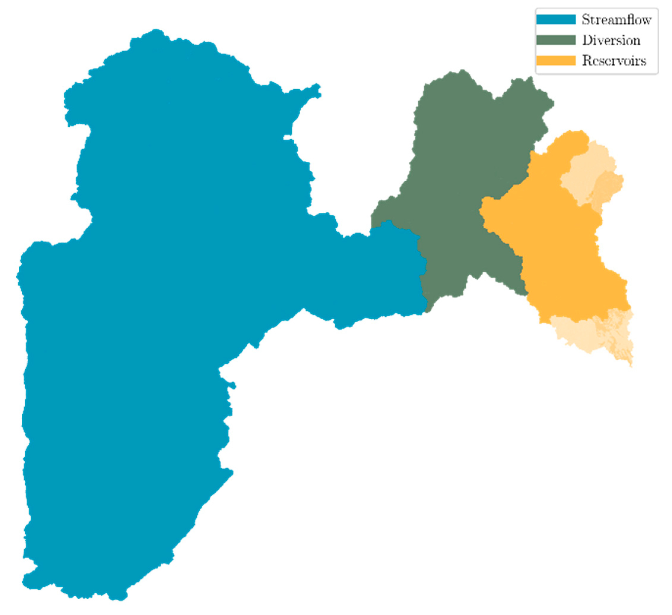
• When analyzing the simulation setup, it is important to differentiate between drainage areas dominated by streamflows, diversions, and reservoirs (see Figure 5). In the case of drainage areas with reservoirs, a simulation was needed for each, though PRMS allows the simulation of up to four reservoirs at once. One subbasin was needed for each diversion since water transfers were implemented to the entire subbasin and taken out of the resulting subbasin outflow. For the case of streamflow, all could be simulated at once and there was no need to split the simulation based on the number of stream gages, as illustrated in Figure 5.

2.

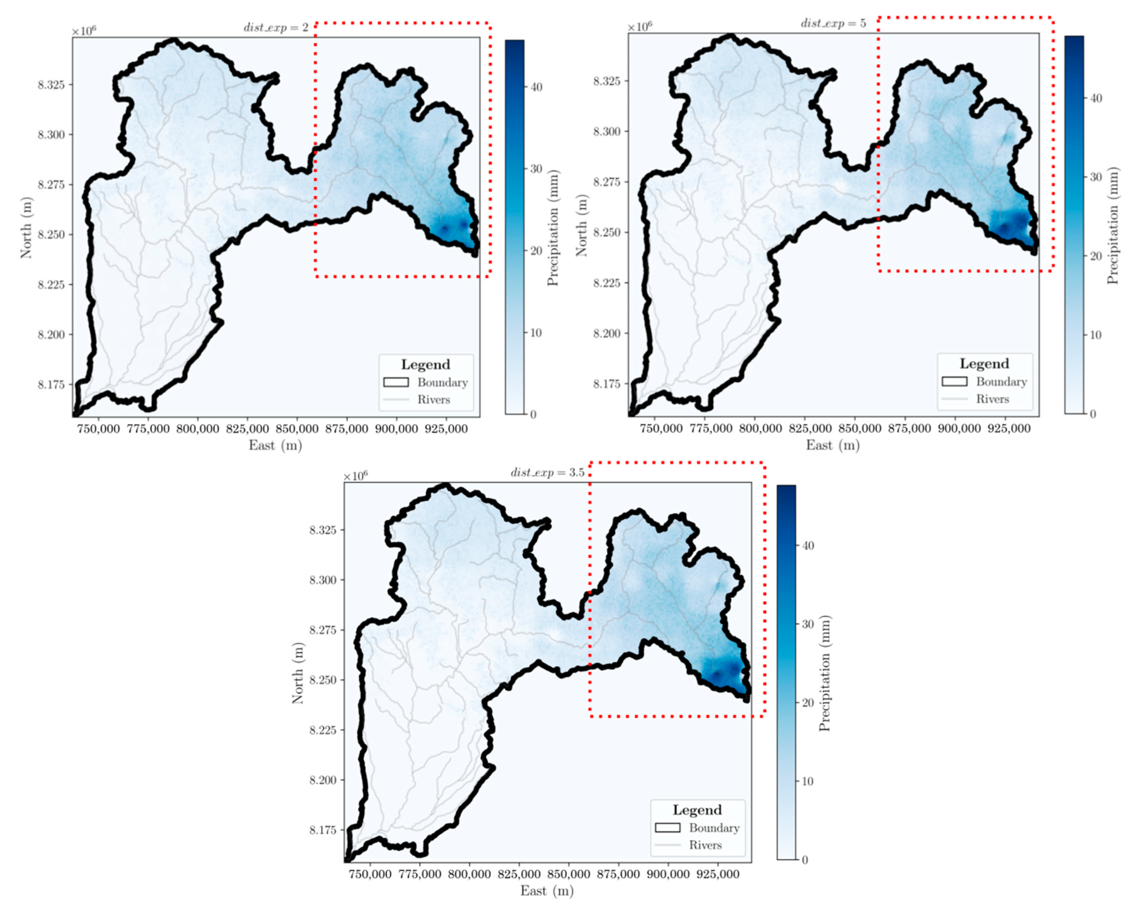
To speed up the simulations, climate files for each one of the five watersheds were created. Three main variables are dominant in the inverse distance-elevation weighting (IDE) method of PRMS, from which two main variables were adjusted. The first variable (“dist_exp”) is the most important since it provides more weight in the spatial distribution for a certain weather station, while the second one (“prcp_wght_dist”) is a ratio to adjust more weight to distance or elevation, from which 75% percent of weight was given to distance and 25% to elevation. The problem with elevation was the drastic changes in the characteristic topography of the Peruvian Andes, which caused a lot of “noise” in the distribution. To test the first variable, a gridded HRU approach was applied to smooth the distribution of the climate variables. The gridded approach allows seeing a proper distribution of the climate variables compared to the semi-distributed one that is used for the models. The “dist_exp” variable is highly sensitive (i.e., the higher its value, the more influence the weather stations will have in nearby cells). Many values were tested for this parameter and a value of 3.5 was chosen since it smooths the distributions best (see Figure 6). The same values were applied to the five watersheds and Climate by HRU (CBH) files were created.

Considering surface outflows (and not reservoir calibration), in the Camana watershed the only area with a different simulation starting date than listed above was the Bamputañe reservoir, which was built in 2009. Therefore, there are three years in which the Bamputañe reservoir would be providing flows to the Condoroma reservoir but are not included in the simulation, which is estimated to be negligible since the storage in the latter is significantly higher. In the case of the Quilca watershed, the starting period of the Aguada Blanca reservoir (located downstream of the other three reservoirs) is affected by the construction year of the upstream-located reservoirs Pillones (in 2007) and Challhuanca (in 2009), but this does not affect the downstream gages from it since there were data available for its outflows since 2006. The Tambo watershed was the one that had the longest simulation period, while the Yauca watershed had only three years of data (gathered by an irrigation association), so the distribution of the data was poor. Furthermore, the Ocoña watershed also had a bad overage for the simulated periods.

Before mentioning the calibration results, it is relevant to define which data were most important for certain watersheds, based on our literature search and information gathering. For instance, since the Yauca watershed has only one stream gage, this gage is extremely relevant for this watershed. The situation is different for the other watersheds; it depends on whether there are reservoirs present or just stream gages. In the case of streamflows, the flows vary depending on the season (dry or wet), so both seasons are analyzed, defining a dry period from May to November, and a wet period from December to April. In the case of reservoirs’ surface outflows, only scheduled releases were evaluated. Additional relevant information for the Ocoña, Camana, Quilca, and Tambo watersheds is described below:

-

The Ocoña watershed has only two stream gages. The Ocoña stream gage is more important since it is located in the lowest elevation, representing a larger portion of the watershed. The Salamanca stream gage contributes around 11 and 4.5% for the dry and wet seasons, respectively.

-

For the Camana watershed, the Pañe, Bamputañe, and Dique reservoirs only contribute their spillway flows to the Camana watershed, which is negligible for a given year since it only happens sometimes during the wet season. Condoroma outflows, on the other hand, are highly tied to streamflow measurements in Tuti; Condoroma outflows are 74 and 22% of the Tuti flow for the dry and wet seasons, respectively. Since the Tuti stream gage diverts a big portion of its flows to the Quilca watershed, it contributes more water to the Huatipa station during the wet season (50%) than during the dry one (2%). Additionally, there is a flow loss of around 29% from the Huatipa to the Hacienda Pampata stream gages during the dry season, which could due to a shortage of data in the Hacienda Pampata time series. Huatipa, on the other hand, contributes 73% of Hacienda Pampata flows during the wet season.

-

In the Quilca watershed, some external inputs come altogether through the Zamacola channel. The Pañe, Bamputañe, and Dique los Españoles reservoirs contribute 41%, 18%, and 10.35%, respectively. It is important to acknowledge that there are unknown flows from some intakes along the Pañe-Colca channel. The Zamacola channel contributes to the Sumbay stream gage with 82% and 69% for dry and wet seasons, respectively. Moving downstream to the Aguada Blanca reservoir, 53%, 6%, 12%, and 23% of the regular discharges from the reservoir are contributed by the Sumbay, Challhuanca, Pillones, and Frayle diversion/reservoirs, respectively. The last two stream gages in this watershed are the Tingo Grande and Puente del Diablo; it is hard to compare the flows downstream on Puente del Diablo with the Aguada Blanca releases since there are some water uses associated with this stream. There is a flow loss of 30% during the dry season, while for the wet season a one-to-one relationship was found. Meanwhile, for the Tingo Grande flow recording station, there is a contribution of 2% and 8% for the dry and wet seasons, respectively.

-

For the Tambo watershed, 1% and 3% are contributed for the dry and wet seasons, respectively, between the Pasto Grande reservoir and the Santa Rosa stream gage.

From the calculated relationships, it can be seen that: (1) for the Ocoña watershed, the Salamanca stream gage does not have an important contribution and the main gage is the Ocoña station; (2) for the Camana watershed, the three upstream reservoirs are only contributing spillway flows to the Condoroma reservoir, and it is mainly used to supply flows for the Tuti diversion. Moreover, a big gap between the Tuti and Huatipa stations was detected, from where the Condoroma reservoir and the Tuti diversion characterize the overall diversion/reservoir infrastructure of the regulated part of this watershed, and the Huatipa and Hacienda Pampata stations represent the unregulated part of the watershed, being the Huatipa station the most important since it catches the flows of the drainage areas that supply most of the water; and (3) for the Quilca watershed, the Pañe reservoir from the Camana watershed supplies most of the water through the Zamacola channel. Similarly, this channel supplies most of the water to the Aguada Blanca reservoir compared to the other three reservoirs that this watershed has (El Frayle, Pillones, and Challhuanca). The Aguada Blanca reservoir is the most important one (in terms of surface outflows) since it regulates the Arequipa city water supply. Moreover, the Puente del Diablo station is located downstream from this reservoir and almost at the southernmost point of the city. For this station, the most important contribution is given by the Aguada Blanca reservoir outflows.

3.2.3. Model Calibration

The main runoff-related variable adjusted was “carea_max” (see SI 3), which specifies the percentage of the HRU that produces runoff. The other main variables represent the region between the soil zone and groundwater, which were the most complex. The soil zone included a capillary reservoir (amount of water held in soil moisture), gravity (mobile in the soil zone), and preferential flow (PFR) storage (not included). Hence, after getting familiar with each watershed and how water is managed on them, a conceptual map (see Figure 7) for these storages was prepared to guide the calibration.

The sensitivity analysis varied depending on the target observation and subbasin. Evaporation rates were not analyzed for sensitivity since one variable was available to adjust. Moreover, a critical factor for the sensitivity results was the boundaries applied to each sensitivity analysis. Overall, the model output was most sensitive groundwater parameters. Figure 8 shows an example of a sensitivity analysis where the metric to be evaluated was the total sensitivity index, with the model output being most sensitive to “gwflow_coef” and “gwstor_min” (the first parameter adjusts the baseflow rates and the second one adjusts the minimum groundwater storage to be preserved in the subbasin).

The time series for each observed dataset was calibrated. Figure 9, Figure 10 and Figure 11 represent examples of calibrated time series for evaporation, reservoir volumes, and streamflow, respectively. Reservoir volumes and streamflows are in English units since it is the default model output for PRMS, as previously mentioned. Moreover, evaporation calibrations got Nash–Sutcliffe Efficiency (NSE) greater than one and very low Root Mean Squared Error (RMSE) since the calibration was performed based on monthly means and there was only a need to adjust one evaporation parameter for each month. A complete view of all calibrated datasets for reservoir evaporation, reservoir volumes, and streamflows are shown in SI 4, SI 5, and SI 6, respectively.

RMSE in the calibrations has many magnitudes and it changes between simulations depending on the minimum and maximum observed records. This statistic was helpful to reduce errors when NSE could not be improved. Starting dates of simulations, the percentage of data available, and the calibration statistics can be seen in

Table 4. Calibration statistics, simulation starting dates, and the percentage of data available for calibration for each subbasin.

Watershed	Subbasin Simulation	Starting Date (d/m/y)	Data Available from Starting Date to End Date (%)	NSE	RMSE
Yauca	Yauca	1 January 2014	51	0.56	9.43 m3/s
Ocoña	Ocoña	1 January 2001	29	0.73	57.88 m3/s
Ocoña	Salamanca	1 January 2001	59	0.35	2.02 m3/s
Camana	Pañe (reservoir)	1 January 2006	100	0.8	12.27 hm3
Camana	Bamputañe (reservoir)	1 February 2010	100	0.73	6.32 hm3
Camana	Dique los Españoles (reservoir)	1 January 2006	100	0.15	2.64 hm3
Camana	Condoroma (reservoir)	1 January 2006	100	0.8	29.95 hm3
Camana	Tuti (diversion)	1 January 2006	100	0.87	17.33 m3/s
Camana	Huatipa	1 January 2006	67	0.86	44.92 m3/s
Camana	Hacienda Pampata	1 January 2006	52	0.63	45.44 m3/s
Quilca	Challhuanca (reservoir)	9 January 2009	100	0.83	3.30 hm3
Quilca	Pillones (reservoir)	10 January 2007	100	0.98	3.23 hm3
Quilca	El Frayle (reservoir)	1 January 2006	100	0.75	280 hm3
Quilca	Aguada Blanca (reservoir)	9 January 2009	100	-46.6	41.14 hm3
Quilca	Sumbay	1 January 2006	100	0.79	2.69 m3/s
Quilca	Puente del Diablo	1 January 2006	53	0.67	6.23 m3/s
Quilca	Tingo Grande	1 January 2006	63	0.74	1.01 m3/s
Quilca	Pitay	1 January 2006	100	0.72	2.77 m3/s
Tambo	Pasto Grande (reservoir)	1 January 1997	99	0.6	20.33 hm3
Tambo	Santa Rosa	1 January 1997	97	0.71	1.37 m3/s

.

While most sub-basin calibrations had great fits, it was not possible to calibrate some of them since there was occasionally missing or insufficient data. Furthermore, for some reservoirs such as Challhuanca and Aguada Blanca, the spillways were not used since they dried the reservoirs when simulated. The Tambo reservoir did not have a precipitation gage, which means that the calibration only relied on the Peruvian Interpolated data of the SENAMHI’s Climatological and hydrological Observations (PISCO) dataset. Three calibrations were considered unsuccessful (detailed below):

-

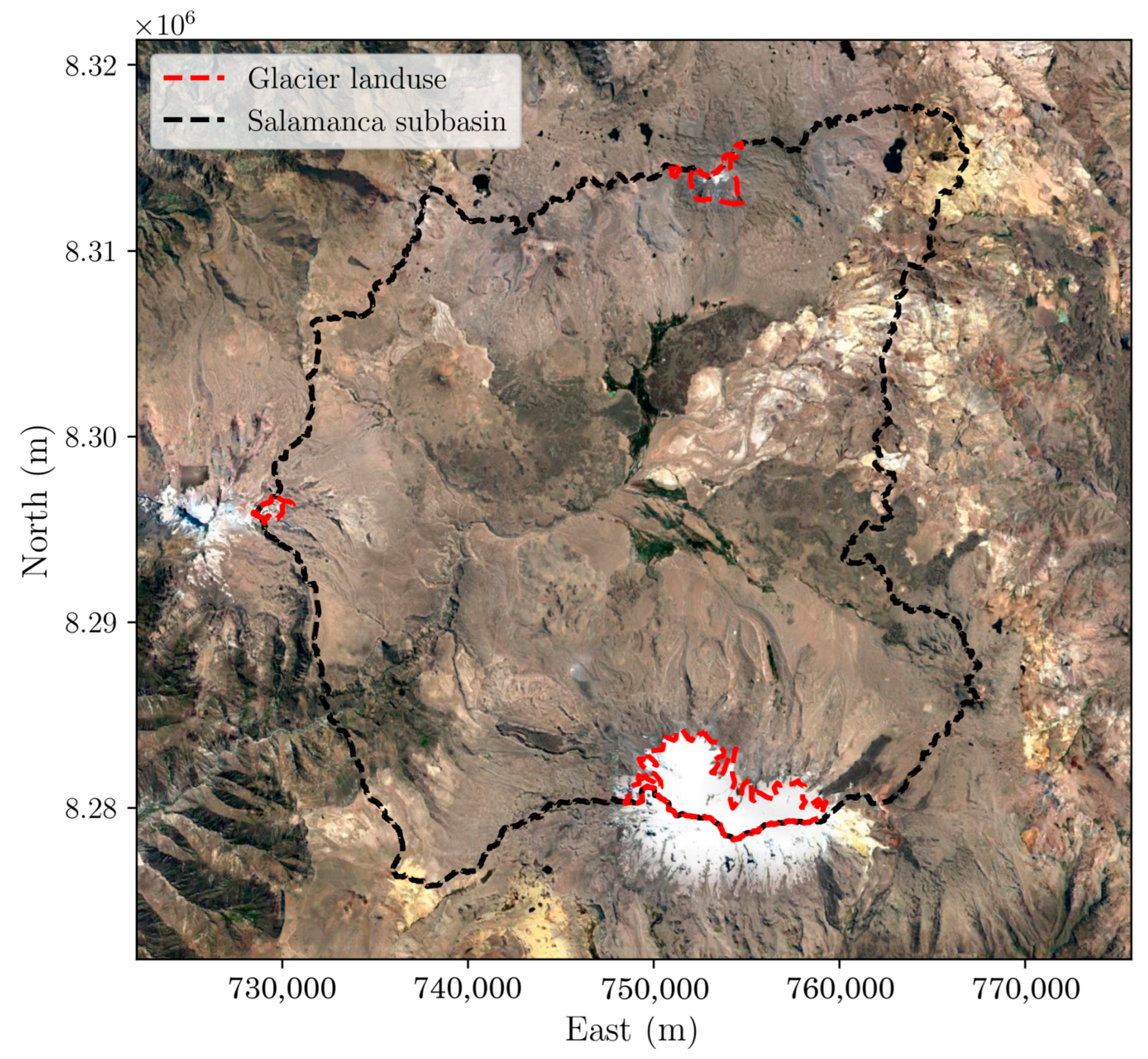
The Salamanca subbasin, located in the Ocoña watershed, from which an NSE of 0.35 was obtained, though only a small percentage of importance was associated with the main stream gage. There was not enough data to catch the dry seasons and, more importantly, different baseflow magnitudes during the dry seasons. The hypothesis associated with this is that this stream gage is located downstream of a glacier (see Figure 12), which by having different melting periods is changing this dynamic. Moreover, some previous studies (e.g., [34]) have tried to calibrate this stream gage but were not successful and lesser performance (NSE = 0.20). A study developed by ANA had better results but the simulation was developed on a monthly basis [22].

-

For the Dique los Españoles reservoir, an NSE of 0.15 was achieved. The problem faced in this reservoir was missing inflows from the hydraulic infrastructure surrounding the structure, and probably high groundwater flows since there is a nearby lagoon. Also, there are missing records from the Jancolacoya and Antasalla water intakes (see Figure 2).

-

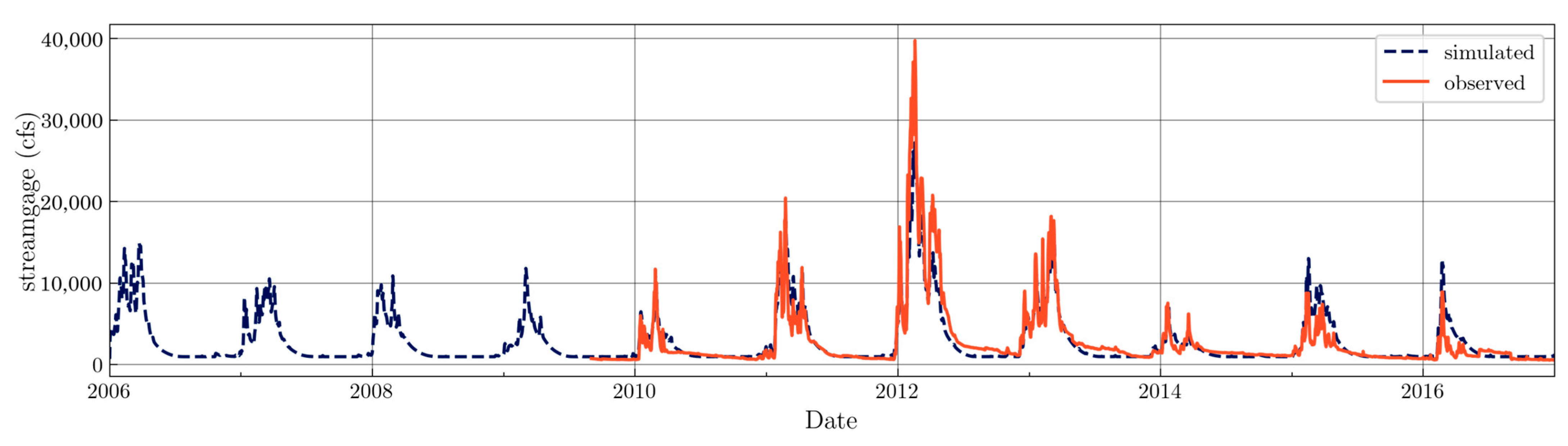
The Aguada Blanca reservoir had the worst calibration statistics. Poor calibration was since the downstream flows coming from the Pillones Tunnel were not recorded, so mass balance errors were obtained when trying to do a mass balance between the flows of the Sumbay stream gage (which is located not so far upstream from the Pillones Tunnel diversion) and the flows being diverted to Pillones. The second and most important reason is the dataset for spillways, from which AUTODEMA and EGASA had different records. Furthermore, when activating the spillway flows, the reservoir volume decreased to zero. Some hypotheses for this could be as follows: (1) higher flows are coming from the Pillones reservoir; (2) the precipitation distribution needs more stations in the drainage area contributing to the reservoir inflows; and (3) the spillways are wrongly measured or summarized, since giving one uniform flow for the spillways for an entire day dried the reservoir, and it is not the same to have a high discharge for 24 h and just for six hours. The year 2012 was the most problematic, where a high precipitation event triggered the spillways and the errors (see Figure 13).

3.3. Future Scenarios: Hydrology and Water Usage

3.3.1. Future Scenarios: Hydrology

From all of the available General Circulation Model (GCM) datasets, 13 models were selected for both historic (1940–2014) and future (2015–2100) datasets (see Section 3.1 for details). Three main errors were found in these downscaled GCMs: (1) the minimum temperatures were greater than the maximum ones for certain points near the shoreline of the study area, which is something that also happened with the PISCO dataset (see SI 1); (2) the downscaled points were overestimating precipitation in lower parts of the watersheds, where precipitation is scarce; and (3) for some GCM models, there wasn’t a smooth transition of temperatures when going from historical to future datasets.

A bias correction was performed for each precipitation data value for each dataset (see Figure 14 for an example of one data point). This process is straightforward and allowed us to mitigate over- or under-estimations of precipitation and temperatures, while buffering the dispersion of the parameters.

From the bias-corrected time series of temperatures, most watersheds followed the same increase patterns between SSPs and future years (see Table S1 in SI 7). Temperature changes were similar for each watershed. Hence, an overall projection for the five watersheds was successfully performed, in which mean increases of 0.73 ± 0.06, 1.20 ± 0.41, 2.25 ± 1.12, and 2.73 ± 1.25 °C could be expected for SSPs 126, 245, 370, and 585, respectively.

Weighting precipitation for an entire watershed is complicated since the spatial distribution of precipitation varies, particularly with the extreme topography changes in Peru, where low or zero precipitation is found in the lowest parts of the watersheds and most comes from higher elevations. The same procedure as temperatures were used and precipitation values accounted for an increase between 0 and 0.98 mm/day (see Table S2 in SI 7). The larger value is not negligible when calculating the total flow produced by its drainage area. Of the five watersheds, Camana received highest increment in mean precipitation, while Yauca had the lowest, which is expected due to its topography does not have the high elevations compared to the other watersheds. Summarizing each SSP mean daily precipitation increase, 0.10 ± 0.07, 0.23 ± 0.11, 0.19 ± 0.17, and 0.34 ± 0.27 mm/day could be expected for SSPs 126, 245, 370, and 585, respectively.

In summary, the models predict an overall increase in precipitation and temperature within the study area, with this increase being directly related to the severity of SSPs, agreeing with the findings by other authors (e.g., [35]). With this preliminary analysis in mind, each previously simulated set of subbasins was computed using the future climate change datasets. As previously mentioned, three different analyses were performed, and similar characteristics were found through all simulations for each evaluation. Examples for each analysis were developed for monthly means and yearly cumulative rates, where lines denote the mean of the ensembles represented by bands for each SSP (see Figure 15, Figure 16, Figure 17, Figure 18, Figure 19 and Figure 20). The means were used as a reference since there is a lot of uncertainty among climate change models.

The following discussion uses the Condoroma Reservoir as a typical example of all of the reservoirs. Monthly reservoir evaporation means demonstrate the positive increase in evaporation moving from SSP 126 to 585 (see Figure 15). Moreover, yearly cumulative rates show the same behavior as monthly ones. The mean trend is conservative for years before 2050, but after that the discrepancies between SSPs are evident (see Figure 16). There is also a discrepancy in the cumulative time series between historic and future datasets, which might be due to the fact that not enough historical data were available.

When analyzing reservoir inflow mean changes (see Figure 17), high flows are identified during the wet season and no substantial changes are simulated for the dry season. Moreover, the change in the mean inflows is not as pronounced as the overall change for the ensembles. When analyzing yearly cumulative inflows (see Figure 18), the same tendency as for evaporation is found, where the total volumes per year for each reservoir increase proportionally to SSP scenario. However, here the ensembles show a much higher uncertainty when dealing with higher SSP levels.

The following discussion for stream flow uses the Tuti stream gage as a typical example. Streamflows exhibit similar behavior as reservoir inflows for both monthly means (see Figure 19) and annual cumulative flows (see Figure 20), with the only difference being related to the stream gage altitude. The monthly means could have a longer dry period compared to the one shown in reservoirs, which are normally located in the highest elevations and where it rains the most. Since stream gages are all connected when no reservoirs are present, this could modify the downstream stream gages’ dry periods since flows could be produced in high-elevation areas.

In all yearly cumulative time series, it is easy to see that the trends of climate change vary significantly, but this change is pronounced towards extreme values; minimum values are buffered and the tendency for the four analyzed SSPs is similar. Future evaporation projections were conducted for all reservoirs except Pasto Grande (Tambo watershed) since no observed records were available, as previously mentioned. The trends for each reservoir are similar; the increase is directly proportional to the previously analyzed gradient of future temperatures. The maximum increases for the year 2100 (with respect to the year 2025) range between 1–3, 1–10, 12–19, and 17–22% for the SSP 126, 245, 370, and 585, respectively (see Table S3 in SI 7). Reservoirs located in the Quilca watershed have the highest increases in evaporation but, as previously mentioned, the increased ranges do not vary a lot from one dataset to another, so the increases in evaporation could be more associated with the latitude and longitude from where reservoirs are located; the highest altitudes in the watersheds have the lowest temperatures which can mitigate evaporation. Moreover, the Aguada Blanca reservoir, which is considered one of the most important reservoirs for the Quilca watershed, has the highest evaporation rate increases, and it is the most downstream reservoir.

Moving forward to reservoir inflows, the increase for the year 2100 (with respect to the year 2025) are 4–42, −1–43, 75–152, 78–216% for the SSP 126, 245, 370, and 585, respectively (see Table S4 in SI 7). From these values, the lowest relative increase is for the Tambo reservoir and the highest is at the Condoroma reservoir. Similar behaviors are presented when analyzing the total volumes for each reservoir. The Condoroma reservoir is still the one that would have the biggest changes in the future, reaching maximum increases of 2217 hm³ for the year 2100. Pasto Grande is not the one with the lowest volumes but, as previously mentioned, the relative change is the lowest for this reservoir. Moreover, besides Condoroma, reservoirs such as Pasto Grande, Pañe, Aguada Blanca, and El Frayle are the ones with the biggest volume changes. There are multiple possible answers for these changes and specific reservoirs would require further analysis. For instance, the Aguada Blanca reservoir has low storage compared to the other reservoirs, but its drainage area is large. The Pañe reservoir, on the other hand, has a small drainage area but its flows would increase considerably. Some relationships could also be performed based on their designed storage, from where Condoroma, Pasto Grande, and El Frayle stood out.

Regarding streamflows (see Table S5 in SI 7), the increase with respect to 2025 is 17–29, 20–59, 118–457, and 144–704% for SSPs 126, 245, 370, and 585, respectively. It is seen that the increases are greater than in the previous analysis, but this increase is not uniform throughout the watersheds. The biggest increases are found in the Puente del Diablo and Tingo Grande subbasins, from where Tingo Grande is inside the drainage area of the Puente del Diablo streamgage. Hence, these increases could be due to errors regarding the climate change datasets for the Tingo Grande drainage area since there are no known parameters or conditions that could be generating this huge change apart from the natural groundwater influence seen in this subbasin [21]. Thus, Tingo Grande is thus highly uncertain and needs further assessment.

Furthermore, the Pitay and Sumbay stream gages, which are the two subbasins with diversions, have the lowest flow increases through the four analyzed SSPs, meaning that in the future these subbasins would still rely on diversions. While methods such as unitary flow are available to compare flows in different sub-basins, it is complicated to compare predicted subbasins’ streamflows since these are highly tied to reservoirs’ operations, which is the main reason by which the analysis was performed per sub-basin or set of sub-basins; moreover, it is not possible to know future reservoir operations. Hence, the flow magnitudes presented in Table S5 in SI 7 should be carefully considered for management purposes since it is shown that simulated results regarding streamflows are more uncertain than previous analyses. It would be useful to analyze the surface-groundwater interactions for each subbasin to reduce this uncertainty. It may also be useful to include evaluating the influence of glaciers in these basins. For the results presented, the Ocoña watershed will be the one with the highest flow increments, followed by the Camana, Tambo, Yauca, and Quilca watersheds. This assumes that the reservoirs would be able to store all of the documented flows, which may not be true knowing the actual reservoirs’ capacities. Hence, in case of reservoir failure, Quilca could move to the third position. Additionally, it is known that some of the reservoirs in the region, Pasto Grande for example, is decreasing in volume due to sediment infilling [36,37]. To date, no plan exists to remediate this loss of reservoir volume. Thus, reservoirs may not be able to store these increased flows.

There is a linear relationship between SSP and future years. In other words, it could be expected to have similar flows for the year 2100 in SSP 370 compared to the year 2075 and the SSP 585. Moreover, lower SSP scenarios such as SSP 126 tend to preserve maximum flows over time.

3.3.2. Future Scenarios: Water Usage

Current water usages vary among watersheds [20,21,22,23,24,25,26,27,28], with agriculture exhibiting the highest demand. The other usages (potable water for populations, mining, and industry) are considerably lower (see Figure 21, note logarithmic scale). It is difficult to apportion future water usages accurately in each watershed, as discussed below, but by employing some simplifying assumptions, a useful analysis can be presented.

Based on migration studies, substantial population increases are expected only in certain areas: the urban areas surrounding the city of Arequipa, and areas associated with agriculture, particularly large agricultural projects such as Majes [38]. The rest of the regions had negative or very low migration rates for the recent 2017 census, so population increases are not expected for most watersheds. Population increases are expected mainly in the Quilca watershed [38]. However, future population increases cannot be accurately evaluated. For example, the largest cities in each watershed might demonstrate increases in population. Peru is concerned about population migration to the urban areas, so the country is likely to implement some solutions that could mitigate this migration.

Increases in population could have serious impacts on water availability. Thus, four different scenarios based on the total demand were applied to the current water uses shown in Figure 21. The scenarios consisted of increases in the overall water demand per watershed, from where increases equivalent to 25%, 50%, 100%, and 200% were applied. The only watershed with expected problems would be Yauca; if it’s demand triples, water needs would exceed supply (assuming all of the additional summer-season flows could be captured and stored). However, this large increase in demand is unlikely due to the fact that, currently, the area experiences negative migration rates [38]; it is a remote watershed that is not expected to see many increases in population, and no major agricultural projects exist in this area (i.e., small-scale or family farming dominates).

Some water shortages might be expected in the watersheds if demand increases excessively. For example, if demand increases by 300% in the region, the demand will exceed supply, causing a shortage. However, excessive increase, while not expected, could be balanced with new ways to improve water storage capacity. For example, storage capacity (reservoirs) should be maintained, i.e., sediment accumulation in reservoirs needs to be evaluated (something that has not been carried out, as previously mentioned) and controlled, if needed. Indeed, sediment accumulation is the biggest problem that reservoirs face around the world, resulting in a worldwide loss of around 20% storage capacity [39], also decreasing the lifespan of the structures. There are ways to prevent this from happening in Arequipa (see [40]). In general, the best way to avoid sediment problems in reservoirs is to build the dam in the right place (location). A small reservoir on an extremely muddy river will rapidly lose its capacity, but a large reservoir on a very clear river may take centuries to lose an appreciable amount of storage. The key factor relies on choosing watersheds that naturally release the least quantity of sediments, i.e., watersheds in good hydrological conditions. For the Arequipa case, the lack of vegetation in the arid environment means that significantly more sediments are being transferred into the reservoirs during storm events. Despite the above, if the dam was already built and sediment deposition needs to be evacuated (as is most likely the case for the Arequipa region), there are effective strategies and techniques that can be applied. The problem of sediment accumulation in reservoirs can be handled in three different locations: (1) in the watershed, using known techniques such as slope stabilization and waterway sediment control, a particularly expensive solution for the study area, considering site conditions; (2) in the reservoir, the most appropriate approach for Arequipa, represented by dredging, flushing, hydrosuction, and the avoidance of settling of fine sediments. Though the approach is normally expensive, it could evacuate a significant portion of deposited sediments downstream; and (3) at the dam using techniques such as dam heightening, sluicing, and turbidity current venting. Considering all of the above, a technical-economic evaluation will be required to decide which approach (or combination of them) should be used to ensure enough storage capacity of reservoirs, based on future conditions.

In addition to the above, the models suggest high flow generation during wet seasons, significantly higher than present day flows, not only in the Department of Arequipa, but also in most of the lower sub-watersheds draining to the Pacific Ocean. The phenomenon is locally known as “huaycos”, which are a constant threat to water availability, water quality, and the population’s welfare [3]. While beyond the scope of this water resources evaluation, huaycos need to be addressed with the necessary structural applications to prevent future disasters. Furthermore, our data analysis indicates that once the capacity of the reservoirs is reached (which can occur early in the wet season), the remaining entering water is simply evacuated downstream, which explains why local rivers still increase their flow rates for months during Peruvian summers, even though there are reservoirs built upstream. Even if a small portion of that water was stored, that would increase the availability of the resource for other uses. Storage capacity alternatives are a function of social, ecological, and economic variables, and are represented mainly by the construction of new reservoirs and the implementation of aquifer recharge facilities. However, both options require further scientific evaluation. This improved storage will be especially important during the dry season; according to model simulations, flows do not increase during those periods, but evaporation increases, reducing reservoir storage, which means increases in the future demands during this season could result in water shortages, particularly for unregulated sub-watersheds (i.e., watersheds without reservoirs). The scenario is likely due to the fact that agriculture occurs year-round in southern Peru and domestic water usage does not decrease during dry seasons. Hence, there is a critical need to increase storage in the unregulated watersheds as well as the regulated ones; specifically, storage that can capture the free flow of water during the wet season, wherein the water supply is most affected by climate change.

Given the uncertainty of future demands, improving irrigation efficiency would be prudent, as crop’s evapotranspiration will increase, according to model simulations. Irrigation efficiency is defined as the amount of water used by crops, compared to total water applied through irrigation (e.g., [41]). The highest irrigation efficiency reported in the five watersheds is 0.77 for the sprinkling irrigation system of Majes [16]. However, the dominant irrigation in the five watersheds is traditional gravity (flooding) methods, which have lower efficiencies (e.g., [42]). If irrigation efficiencies similar to the ones at Majes should be reached, an increase of the efficiency would be needed; this reduced use would likely never exceed demand due to the fact that agricultural water use dominates the domestic water used by the population; population demands are just 0.42%, 0.54%, 0.54%, 13.19%, and 1.03% of the agricultural demands for the Yauca, Ocoña, Camana, Quilca, and Tambo watersheds, respectively. Moreover, high irrigation efficiencies could only be reached with technologies such as CIMS (California Irrigation Management System), which provides water to meet actual crop demand based on a dense network of weather stations. Our model calculations indicate that such savings would account for a total of 90, 191, 368, 211, and 163 MCM for the Yauca, Ocoña, Camana, Quilca, and Tambo watersheds, respectively. For the Camana watershed, the savings would account for storage greater than its Condoroma reservoir. Similarly, water-retaining polymers could dramatically decrease irrigation demands if applied at a large scale. For instance, it has been found that polymers could increase water retention by 60% in arid and semiarid regions [43].

The previous discussion promotes a bright outlook for sustainable water resources in the Arequipa region, though the discussion relies on the assumption that the additional water could be stored, or water consumption could be decreased with efficient practices.

Water uses such as diversions or reservoirs outflows were not considered when analyzing climate change scenarios and water uses against climate change scenarios, since these flows are controlled by the operators. This means that the analysis reflects the possible changes inside its drainage area (sub-basin). Moreover, groundwater was not considered because of the lack of available records (most uses are based on surface water flows and storage). For example, in the Quilca watershed, agricultural water demands associated with diversions such as the Majes, Pampa de Siguas, and others inside the drainage area of the Pitay stream gage were not considered since those heavily depend on the diversions coming from the Camana watershed. Any specific demands with calculations associated with groundwater were subtracted or not considered in the analysis if not found.

Our approach also has limitations since water demands have spatial variability. For example, mining in some watersheds is concentrated in high-altitude areas, while agriculture could be associated with middle-lower terrains. Similarly, it is important to highlight that our analysis did not include environmental water needs, as there was no information available for this important topic. Future studies should follow the methods applied by other authors that have considered the ecological factor as part of their analyses (e.g., [44]).

4. Conclusions and Recommendations

For the first time, the Arequipa Region of southern Peru has been characterized and evaluated in terms of water management, after extensive analysis consisting of gathering information from private and public entities to build and calibrate a hydrological model, providing an important tool for future management decisions, thus ensuring sustainability of surface water resources.

After carefully analyzing climate change predictions with the ensembles for each SSP, all reservoirs and stream gages in the studied watersheds show the same trend: a clear increase in flows during wet seasons and no substantial changes during the dry seasons.

Evaporation generally increases due to higher temperatures but there is significant uncertainty in the rates derived from the future climate data. The increase is directly proportional to the SSP level under consideration and has similar magnitudes for all months, which is a different behavior than that predicted for flows, and the resulting loss of stored water could trigger significant deficits during dry seasons if not managed correctly. Therefore, reservoir storage (i.e., sediment deposition) would need to be further assessed since the entire Arequipa Region relies on reservoirs to supply water for all uses in the future.

Most importantly, considering both climate change and hypothetical future demands for the five watersheds, there will be water available to satisfy annual demands, but since most of the flows come during the wet season (when reservoirs currently overflow during peak flows) an increase in watershed storage capacity and irrigation efficiency is strongly recommended to ensure future water sustainability, especially during the dry seasons. Similarly, future studies should consider environmental water demands to ensure healthy aquatic ecosystems in the region, following the analysis by Li et al. [44].

Additionally, this study revealed several important deficiencies that need to be addressed to improve water resources management (and sustainability) evaluations in the Arequipa Region:

-

There is a clear need to have a unified database for all weather-related variables, streamflows, and reservoir data. It has been found that entities such as ANA, National Meteorology and Hydrology Service (SENAMHI), AUTODEMA, and EGASA, among others, have different datasets and the data are not compiled into one master repository. This causes many problems such as not accounting for weather stations from reservoirs included in the PISCO dataset and discrepancies between databases from one entity to another. Similarly, it is important to have the data publicly available in a quality assured and organized format, to ease the difficulty of future analyses. Moreover, information gathered by private entities should also be included and made available to the public. These improvements in data management would be a step forward toward achieving sustainable development not only in the Arequipa Region but also in the entire country.

-

For modeling purposes, it is important to include solar radiation measurements in weather stations, especially in areas such as reservoirs and irrigation fields where evaporation and evapotranspiration are a critical piece of the water storage and use evaluation.

-

The inclusion of a weather station in the Pasto Grande reservoir would highly improve conceptualization and modeling of this reservoir.

-

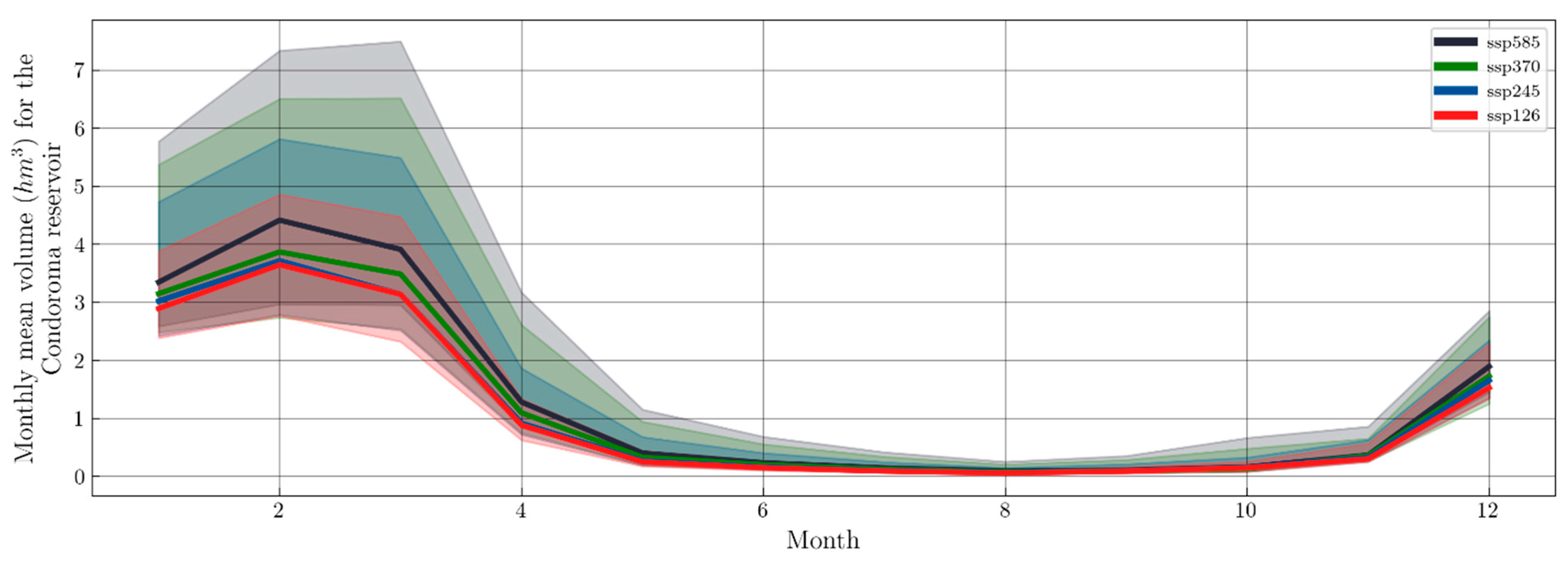
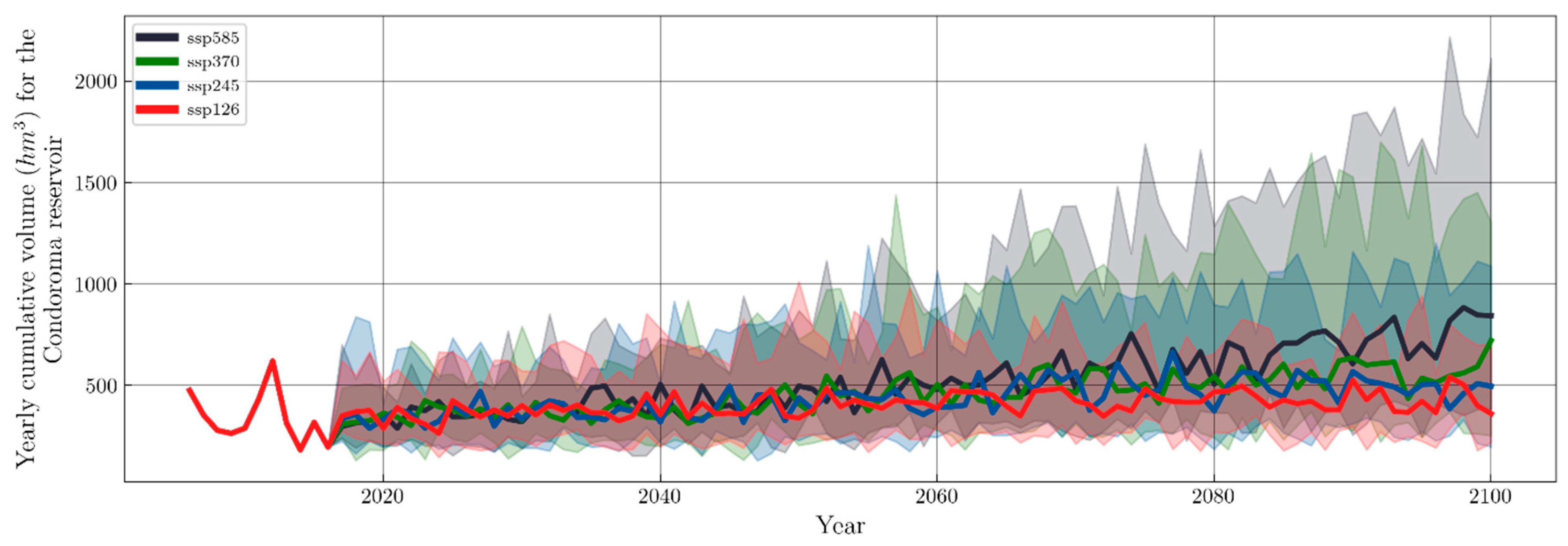
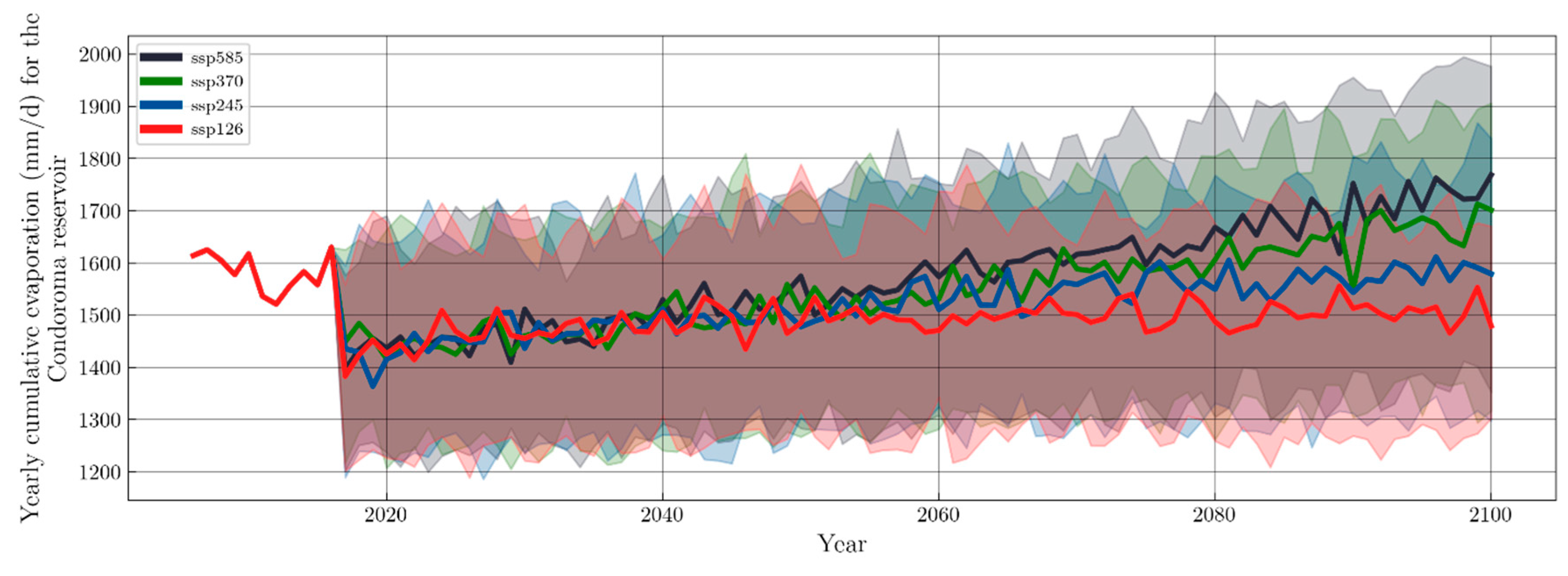
Based on the climate change analysis, reservoirs such as Condoroma, which buffers all inflows coming from the upstream parts of the Camana watershed, may not be able to mitigate the high flows predicted for SSPs higher than 126. In other words, if the Arequipa Region does not follow the conservative SSP, flooding-related (such as fluvial floods and “huaycos”) problems downstream of the reservoirs could worsen, which is something that has been threatening many communities within sub-watersheds draining to the Pacific Ocean.

-

It is encouraged that the PISCO dataset has continuous development. This dataset may not be as accurate as hard data from weather stations but is a product with a good spatial resolution for Peru, derived from raw weather stations data. Moreover, the inclusion of an integrated database, as previously mentioned, would improve its accuracy.

-

Given the strong topographical characteristics of Southern Peru, it is recommended to improve the weather stations’ density and data recording, specially in areas where high water storage is present (i.e., reservoirs and their drainage area).

-

During model calibration, spillway flows produced unrealistic behaviors for some reservoirs. Thus, it is recommended to record hourly time series of spillway flows since the high magnitude of these flows is not usually constant for an entire day, which made some reservoirs go dry as soon as they were activated.

-

Irrigation could be included in the PRMS setup. Land uses associated with irrigation have an HRU identifier. Hence, its inclusion would not be complicated. However, to accomplish this, it would be necessary to monitor irrigation schedules and parameters such as soil moisture and aquifer levels below irrigated areas, which is not currently carried out. Moreover, if an aquifer is generated due to intensive irrigation as in the Majes irrigation district (see [16] for more details), a network of piezometers would be needed to include the groundwater flow direction into the simulation, or more advanced models such as MODFLOW [45] could be linked.

-

It would be useful to include local water consumption for usages such as drinking water in the city of Arequipa, but at least a monthly time series would be needed for each included water use. Currently, estimates for use lack sufficient detail for detailed analyses (for example, to enable a focus of future water supply versus demand monthly during the dry season).

-

If it is desired to improve reservoir dynamics, for instance, to use water levels in the reservoirs for model calibration), which could significantly improve reservoir response and dynamics, PRMS source code would need to be modified to include rating curves of volume versus elevation. This approach would be beneficial if there was a strong interaction between reservoir and surrounding aquifer or if there were seasonal changes in the surrounding aquifer’s water levels, which would allow the model to analyze the elevation at which water in the reservoirs starts to seep into groundwater storage. This approach would require a network of piezometers to monitor the water table surrounding the reservoir.

-

After calibrating the five watersheds, the scarcity of data throughout the study areas was evident. A significant amount of data is missing in the reservoir system of the Quilca watershed. There are many water intakes and channels with unknown flows in the Dique los Españoles reservoir and the Pañe-Colca channel. Moreover, only the flows going towards the Pillones tunnel are known and not the ones going downstream to the Aguada Blanca reservoir. Furthermore, implementing a stream gage upstream of the Aguada Blanca would improve calibration and water accounting since the drainage area for this location has been considered to generate high flows. There is a need for a uniform dataset in all reservoirs and diversions since databases had discrepancies. For instance, the Aguada Blanca reservoir showed a difference of around 50 m³/s (in reservoir spillway flow) between two source institutions that documented the same information. For the rest of the watersheds, there are no specific locations but there is a need for more stream gages and stations, and it would be important to have these near cities or irrigation projects to properly evaluate future impacts.

-

It is extremely important to evaluate reservoir sediment deposition against high flows expected with climate change. The actual capacity of the reservoirs is currently unknown, so an evaluation of sediment accumulation is crucial to ensure future water sustainability in the Region. Hydraulic analysis should be performed to evaluate the possible damages to infrastructure and to downstream inhabitants during the increased “huayco” flows.

-

A more comprehensive analysis of available groundwaterin the five watersheds would be highly useful to evaluate watershed storage capacity, since it could serve as an additional water supply in the future. Groundwater may represent an important way to store water in the future.

-

A holistic evaluation of future water supply and storage options is recommended. Such analysis would include evaluating the construction of new reservoirs, the implementation of aquifer recharge facilities, or other solutions such as natural infrastructure (e.g., constructed wetlands), water treatment options such as recycled water and desalination.

References

1. Global Affairs Canada. Addressing Peru’s Climate Challenges with Nature-Based Solutions. Available online: https://www.international.gc.ca/world-monde/stories-histoires/2022/peru-climate-challenges_defis-climatiques-perou.aspx?lang=eng (accessed on 24 November 2022).
2. World Bank Group. Peru, Country, Climate, and Development Report. Available online: https://reliefweb.int/report/peru/peru-country-climate-and-development-report-november-2022 (accessed on 23 January 2023).
3. UNESCO. Peru Faces a Surge of Climate Migrants. Available online: https://en.unesco.org/courier/2021-4/peru-faces-surge-climate-migrants (accessed on 4 January 2023).
4. USAID. Peru Climate Change Fact Sheet. Available online: https://www.climatelinks.org/resources/peru-climate-change-fact-sheet (accessed on 4 January 2023).
5. The World Bank. Assessment of the Impacts of Climate Change on Mountain Hydrology. Available online: https://documents1.worldbank.org/curated/en/211461468294364190/pdf/ (accessed on 23 January 2023).
6. Lavado-Casimiro, W.; Labat, D.; Guyot, J.; Ardoin-Bardin, S. Assessment of climate change impacts on the hydrology of the Peruvian Amazon-Andes Basin. Hydrol. Process. 2011, 25, 3721–3734. [Google Scholar] [CrossRef]
7. Zubieta, R.; Molina, J.; Laqui, W.; Sulca, J.; Ilbay, M. Comparative analysis of climate change impacts on meteorological, hydrological, and agricultural droughts in the Lake Titicaca Basin. Water 2021, 13, 175. [Google Scholar] [CrossRef]
8. Mishra, A.K.; Özger, M.; Singh, V.P. Association between uncertainties in meteorological variables and water-resources planning for the state of Texas. J. Hydrol. Eng. 2011, 16, 984–999. [Google Scholar] [CrossRef]
9. Irwandi, H.; Rosid, M.S.; Mart, T. Effects of Climate change on temperature and precipitation in the Lake Toba region, Indonesia, based on ERA5-land data with quantile mapping bias correction. Sci. Rep. 2023, 13, 2542. [Google Scholar] [CrossRef]
10. Wang, Y.; Zhang, Z.; Allen, E.E.; De La Guardia, L.; Qie, G.; Wu, X.; Zhao, W. An integrated framework to assess climate change impacts on water use for thermoelectric power plants. J. Clean. Prod. 2022, 376, 134271. [Google Scholar] [CrossRef]
11. Nguyen, T.; Virdis, S.; Vu, T.B. “Matter of climate change” or “Matter of rapid urbanization”? Young people’s concerns for the present and future urban water resources in Ho Chi Minh City Metropolitan Area, Vietnam. Appl. Geogr. 2023, 153, 102906. [Google Scholar] [CrossRef]
12. Orkodjo, T.P.; Kranjac-Berisavijevic, G.; Abagale, F.K. Impact of climate change on future availability of water for irrigation and hydropower generation in the Omo-Gibe basin of Ethiopia. J. Hydrol. Reg. Stud. 2022, 44, 101254. [Google Scholar] [CrossRef]
13. Mendoza, J.A.C.; Alcazar, T.A.C.; Medina, S.A.Z. Calibration and uncertainty analysis for modelling runoff in the Tambo River Basin, Peru, using sequential Uncertainty fitting VeR-2 (SUFI-2) algorithm. Air Soil Áter Res. 2021, 14, 117862212098870. [Google Scholar] [CrossRef]
14. Coloma, A. Simulación Hidrológica e Hidráulica del río Tambo, Sector Santa Rosa, Distrito de Cocachacra, Provincia de Islay, Departamento de Arequipa. Thesis National University of San Agustin, Arequipa-Perú. 2015. Available online: https://core.ac.uk/download/pdf/162860876.pdf (accessed on 2 November 2022).
15. USAID. Quilca-Chili WEAP Model with Refined Strategy. PARA-AGUA Project. Available online: https://pdf.usaid.gov/pdf_docs/PA00N121.pdf (accessed on 3 November 2022).
16. Wei, X.; Garcia-Chevesich, P.; Alejo, F.; García, V.; Martínez, G.; Daneshvar, F.; Bowling, L.C.; Gonzáles, E.; Krahenbuhl, R.; McCray, J.E. Hydrologic Analysis of an Intensively Irrigated Area in Southern Peru Using a Crop-Field Scale Framework. Water 2021, 13, 318. [Google Scholar] [CrossRef]
17. Daneshvar, F.; Frankenberger, J.; Bowling, L.C.; Cherkauer, K.A.; De Lima Moraes, A.G. Development of strategy for SWAT Hydrologic modeling in Data-Scarce regions of Peru. J. Hydrol. Eng. 2021, 26, 05021016. [Google Scholar] [CrossRef]
18. INGEMMET. Hidrogeología de la cuenca del río Quilca—Vitor—Chili (132)—Boletín, Serie H: Hidrogeología, 15. Repositorio Institucional INGEMMET. 2022. 381p. Available online: https://repositorio.ingemmet.gob.pe/handle/20.500.12544/3885 (accessed on 1 November 2022).
19. INEI. Estimaciones y Proyecciones de Población por Departamento, Provincia, y Distrito 2018–2020. Available online: https://www.inei.gob.pe/media/MenuRecursivo/publicaciones_digitales/Est/Lib1715/libro.pdf (accessed on 10 April 2023).
20. INRENA. Estudio Integral de los Recursos Hídricos en las Cuencas de los ríos Acarí y Yauca: Componente—Estudio Hidrológico de la Cuenca del Río Yauca. Instituto Nacional De Recursos Naturales Dirección General De Aguas Y Suelos. Arequipa, Perú. 2003. 84p. Available online: https://hdl.handle.net/20.500.12543/3317 (accessed on 3 November 2022).
21. ANA. Plan de Gestión de Recursos Hídricos en la Cuenca Quilca—Chili. Autoridad Nacional del Agua. Arequipa, Perú.2013. 161p. Available online: https://hdl.handle.net/20.500.12543/10 (accessed on 3 November 2022).
22. ANA. Evaluación de Recursos Hídricos en la Cuenca de Ocoña. Autoridad Nacional del Agua. Arequipa, Perú. 2015. 53p. Available online: https://hdl.handle.net/20.500.12543/8 (accessed on 3 November 2022).
23. ANA. Evaluación de Recursos Hídricos en la Cuenca Camaná—Majes—Colca. Autoridad Nacional del Agua. Arequipa, Perú. 2015b. 840p. Available online: https://hdl.handle.net/20.500.12543/7 (accessed on 3 November 2022).
24. ANA. Estudio Hidrológico de la Unidad Hidrográfica de Tambo. Autoridad Nacional del Agua. Arequipa, Perú. 2019. 208p. Available online: https://hdl.handle.net/20.500.12543/4703 (accessed on 3 November 2022).
25. INGEMMET. Estudio Hidrogeológico de la Cuenca del Río Camaná-Majes-Colca. 2021 Repositorio Institucional INGEMMET. 2021. 280p. Available online: https://repositorio.ingemmet.gob.pe/handle/20.500.12544/3163 (accessed on 3 November 2022).
26. INGEMMET. Hidrogeología de la Cuenca del Rio Tambo (1318). Regiones Arequipa, Moquegua y Puno. 288p. Instituto Geológico, Minero y Metalúrgico—INGEMMET, Lima (Peru). 2020. Available online: https://hdl.handle.net/20.500.12544/2573 (accessed on 3 November 2022).
27. INGEMMET. Estudio Geoambiental en la Cuenca del Río Ocoña. 222p. Instituto Geológico, Minero y Metalúrgico—INGEMMET. 2021. Available online: https://hdl.handle.net/20.500.12544/3167 (accessed on 3 November 2022).
28. SNIHR. Sistema Nacional de Información de Recursos Hídricos. 2022. Available online: https://snirh.ana.gob.pe/VisorPorCuenca/ (accessed on 19 October 2023).
29. Wilson, M.L.; Tchantchaleishvili, V. The importance of free and open source software and open standards in modern scientific publishing. Publications 2013, 1, 49–55. [Google Scholar] [CrossRef]
30. Leavesley, G.H.; Lichty, R.W.; Troutman, B.M.; Saindon, L. Precipitation-Runoff Modeling System; User’s Manual; U.S. Geological Survey, Water Resources Division: Reston, VA, USA, 1983. [Google Scholar] [CrossRef]
31. Quiroz, J.A. Arequipa Watershed-Scale Hydrologic Models, HydroShare. 2023. Available online: http://www.hydroshare.org/resource/d06a41bb8a2f435da6c84792403f961a (accessed on 3 March 2023).
32. Huerta Astorga, J.L. Proyecto Especial Majes Siguas. AUTODEMA Principales Logros Gerencia Gestión de Recursos Hídricos Setiembre. 2011. Available online: https://cdn.www.gob.pe/uploads/document/file/1325831/AUTODEMA%20-%20Audiencia%2001.pdf (accessed on 4 November 2022).
33. Decreto Supremo Nº 002-2008-AG. Reservan Aguas Superficiales a Favor del Proyecto Especial Pasto Grande del Gobierno Regional Moquegua. Diario Oficial El Peruano, 10 January 2008. Available online: https://www.midagri.gob.pe/portal//download/pdf/marcolegal/normaslegales/decretossupremos/DECRETO%20SUPREMO%20N%20002-2008-AG.pdf (accessed on 4 November 2022).
34. Santana, A.D. Elaboración de Modelos Hidrológico y de Gestión en la Cuenca del río Ocoña en Perú y Análisis de Resultados. Master’s Thesis, Universitat Politécnica De Valéncia, Valencia, España, 2018. Available online: https://riunet.upv.es/bitstream/handle/10251/98391/01_Memoria.pdf?sequence=1 (accessed on 2 November 2022).
35. Imfeld, N.; Sedlmeier, K.; Gubler, S.; Marrou, K.C.; Davila, C.P.; Huerta, A.; Lavado-Casimiro, W.; Rohrer, M.; Scherrer, S.C.; Schwierz, C. A combined view on precipitation and temperature climatology and trends in the southern Andes of Peru. Int. J. Climatol. 2021, 41, 679–698. [Google Scholar] [CrossRef]
36. Diario La República. Fuentes de Agua para Ciudades del sur Están en Peligro. 8 Dicember 2019. Available online: https://larepublica.pe/sociedad/2019/12/08/fuentes-de-agua-para-ciudades-del-sur-estan-en-peligro-lrsd/ (accessed on 18 October 2021).
37. Diario El Pueblo. Sedimentación de Aguada Blanca incrementó. 23 March 2016. Available online: https://diarioep.pe/sedimentacion-de-aguada-blanca-se-incremento/ (accessed on 18 October 2021).
38. INEI. Estado de la Población Peruana. Instituto Nacional de Estadística e Informática, 2020. Available online: https://www.inei.gob.pe/media/MenuRecursivo/publicaciones_digitales/Est/Lib1743/Libro.pdf (accessed on 3 November 2022).
39. Perera, D.; Williams, S.; Smakhtin, V. Present and Future Losses of Storage in Large Reservoirs Due to Sedimentation: A Country-Wise Global Assessment. Sustainability 2022, 15, 219. [Google Scholar] [CrossRef]
40. Garcia-Chevesich, P. Erosion Control and Land Restoration; Outskirts Press: Denver, CO, USA, 2016; 486p. [Google Scholar]
41. Xiong, R.; Zheng, Y.; Feng, H.; Tian, Y. Improving the scientific understanding of the paradox of irrigation efficiency: An integrated modeling approach to assessing Basin-Scale irrigation efficiency. Water Resour. Res. 2021, 57, e2020WR029397. [Google Scholar] [CrossRef]
42. Knox, J.W.; Kay, M. Water Regulation, crop production, and Agricultural water Management—Understanding farmer perspectives on irrigation efficiency. Agric. Water Manag. 2012, 108, 3–8. [Google Scholar] [CrossRef]
43. Maghchiche, A.; Haouam, A.; Immirzi, B. Use of polymers and biopolymers for water retaining and soil stabilization in arid and semiarid regions. J. Taibah Univ. Sci. 2010, 4, 9–16. [Google Scholar] [CrossRef]
44. Li, W.; An, M.; Wu, H.; An, H.; Huang, J.; Khanal, R. The local coupling and telecoupling of urbanization and ecological environment quality based on multisource remote sensing data. J. Environ. Manag. 2023, 327, 116921. [Google Scholar] [CrossRef]
45. Hughes, J.D.; Russcher, M.J.; Langevin, C.D.; Morway, E.D.; McDonald, R.R. The MODFLOW Application Programming Interface for simulation control and software interoperability. Environ. Model. Softw. 2022, 148, 105257. [Google Scholar] [CrossRef]
46. ANA, Catálogo de Metadatos. Available online: http://geo2.ana.gob.pe:8080/geonetwork/srv/spa/catalog.search#/home (accessed on 18 October 2022).
47. Aybar, C.; Fernández, C.; Huerta, A.; Lavado, W.; Vega, F.; Felipe-Obando, O. Construction of a high-resolution gridded rainfall dataset for Peru from 1981 to the present day. Hydrol. Sci. J.-J. Des Sci. Hydrol. 2019, 65, 770–785. [Google Scholar] [CrossRef]
48. JAXA. ALOS Global Digital Surface Model “ALOS World 3D-30 m (AW3D30)”. 2017. Available online: http://www.eorc.jaxa.jp/ALOS/en/aw3d30/ (accessed on 2 November 2022).
49. Hengl, T.; De Jesus, J.M.; Heuvelink, G.; Gonzalez, M.R.; Kilibarda, M.; Blagotić, A.; Shangguan, W.; Wright, M.N.; Geng, X.; Bauer-Marschallinger, B.; et al. SoilGrids250m: Global gridded soil information based on machine learning. PLoS ONE 2017, 12, e0169748. [Google Scholar] [CrossRef]
50. Zonificación Ecológica y Económica (ZEE) a Nivel Regional para el Perú. Available online: https://www.minam.gob.pe/ordenamientoterritorial/zonificacion-ecologica-y-economica-zee/ (accessed on 4 October 2022).
51. Thrasher, B.; Wang, W.; Michaelis, A.; Melton, F.S.; Lee, T.; Nemani, R.R. NASA Global Daily Downscaled Projections, CMIP6. Sci. Data 2022, 9, 262. [Google Scholar] [CrossRef]
52. Quiroz, J. Jonathanqv/cmip6d: Climate Change Processor. Available online: https://zenodo.org/record/7311969 (accessed on 22 January 2023).
53. Hoyer, S.; Hamman, J. Xarray: N-D labeled Arrays and Datasets in Python. J. Open Res. Softw. 2017, 5, 10. [Google Scholar] [CrossRef]
54. The Pandas Development Team. Pandas-Dev/Pandas: Pandas on Zenovo Version v2.1.3. Available online: https://zenodo.org/records/10107975 (accessed on 2 February 2023).
55. WMO. Challenges in the Transition from Conventional to Automatic Meteorological Observing Networks for Long-Term Climate Records; World Meteorological Organization: Geneva, Switzerland, 2017; ISBN 978-92-63-11202-6. Available online: https://library.wmo.int/records/item/55812-challenges-in-the-transition-from-conventional-to-automatic-meteorological-observing-networks-for-long-term-climate-records#.XpYEBNIzbcd (accessed on 5 November 2022).
56. Huang, Y.; Bardossy, A. Impacts of Data Quantity and Quality on Model Calibration: Implications for Model Parameterization in Data-Scarce Catchments. Water 2020, 12, 2352. [Google Scholar] [CrossRef]
57. Arnold, J.G.; Moriasi, D.N.; Gassman, P.W.; Abbaspour, K.C.; White, M.J.; Srinivasan, R.; Santhi, C.; Harmel, R.D.; Van Griensven, A.; Van Liew, M.W.; et al. SWAT: Model Use, Calibration, and Validation. Trans. ASABE 2012, 55, 1491–1508. [Google Scholar] [CrossRef]
58. Van Rossum, G.; Drake, F. Python Tutorial. Centrum voor Wiskunde en Informatica Amsterdam, The Netherlands. Available online: https://www.spiraltrain.nl/python-cursus/?gclid=Cj0KCQjwrMKmBhCJARIsAHuEAPSkiDcpCP-VoV1ukp0JUQVba0p6Lj7_CcZSzW-bKVckhkG-DWqrNJcaAvi6EALw_wcB (accessed on 11 November 2022).
59. GRASS Development Team. Geographic Resources Analysis Support System (GRASS GIS) Software, Version 8.0. Open Source Geospatial Foundation. Available online: http://grass.osgeo.org (accessed on 15 December 2022).
60. Zambelli, P.; Gebbert, S.; Ciolli, M. PyGrass: An object oriented Python Application Programming Interface (API) for Geographic Resources Analysis Support System (GRASS) Geographic Information System (GIS). ISPRS Int. J. Geo-Inf. 2013, 2, 201–219. [Google Scholar] [CrossRef]
61. Jordahl, K.; Van Den Bossche, J.; Fleischmann, M.; Wasserman, J.L.; McBride, J.R.; Gerard, J.; Tratner, J.; Perry, M.; Badaracco, A.G.; Farmer, C.; et al. Geopandas/geopandas: V0.8.1. Zenodo 2020. [Google Scholar] [CrossRef]
62. QGIS Development Team. QGIS Geographic Information System. QGIS Association. Available online: https://www.qgis.org (accessed on 12 October 2022).
63. Regan, R.S.; Markstrom, S.L.; LaFontaine, J. HPRMS Version 5.2.1: Precipitation-Runoff Modeling System (PRMS): U.S. Geological Survey Software Release. 2022. Available online: https://www.usgs.gov/software/precipitation-runoff-modeling-system-prms (accessed on 2 October 2022).
64. Regan, R.S.; LaFontaine, J.H. Documentation of the Dynamic Parameter, Water-Use, Stream and Lake Flow Routing, and Two Summary Output Modules and Updates to Surface-Depression Storage Simulation and Initial Conditions Specification Options with the Precipitation-Runoff Modeling System (PRMS); Techniques and Methods; U.S. Geological Survey: Reston, VA, USA, 2017. [Google Scholar] [CrossRef]
65. Markstrom, S.L.; Regan, R.S.; Hay, L.E.; Viger, R.J.; Webb, R.M.; Payn, R.A.; LaFontaine, J.H. PRMS-IV, the Precipitation-Runoff Modeling System; Version 4; Techniques and Methods; U.S. Geological Survey: Reston, VA, USA, 2015. [Google Scholar] [CrossRef]
66. Terrier, M.; Perrin, C.; De Lavenne, A.; Andréassian, V.; Lerat, J.; Vaze, J. Streamflow Naturalization Methods: A review. Hydrol. Sci. J.-J. Des Sci. Hydrol. 2020, 66, 12–36. [Google Scholar] [CrossRef]
67. Larsen, J.D.; Alzraiee, A.; Niswonger, R. Integrated hydrologic model development and postprocessing for GSFLOW using pyGSFLOW. J. Open Source Softw. 2022, 7, 3852. [Google Scholar] [CrossRef]
68. Shen, H.C.; Tolson, B.A.; Mai, J. Time to update the Split-Sample approach in hydrological model calibration. Water Resour. Res. 2022, 58, e2021WR031523. [Google Scholar] [CrossRef]
69. Knoben, W.J.M.; Freer, J.E.; Woods, R.A. Technical note: Inherent benchmark or not? Comparing Nash–Sutcliffe and Kling–Gupta efficiency scores. Hydrol. Earth Syst. Sci. 2019, 23, 4323–4331. [Google Scholar] [CrossRef]
70. Schaefli, B.; Gupta, H.V. Do Nash values have value? Hydrol. Process. 2007, 21, 2075–2080. [Google Scholar] [CrossRef]
71. Čerkasova, N.; Umgiesser, G.; Ertürk, A. Development of a hydrology and water quality model for a large transboundary river watershed to investigate the impacts of climate change—A SWAT application. Ecol. Eng. 2018, 124, 99–115. [Google Scholar] [CrossRef]
72. Bock, A.R.; Farmer, W.; Hay, L.E. Quantifying uncertainty in simulated streamflow and runoff from a continental-scale monthly water balance model. Adv. Water Resour. 2018, 122, 166–175. [Google Scholar] [CrossRef]
73. LaFontaine, J.H.; Hart, R.M.; Hay, L.E.; Farmer, W.; Bock, A.R.; Viger, R.J.; Markstrom, S.L.; Regan, R.S.; Driscoll, J.M. Simulation of Water Availability in the Southeastern United States for Historical and Potential Future Climate and Land-Cover Conditions; Scientific Investigations Report; U.S. Geological Survey: Reston, VA, USA, 2019. [Google Scholar] [CrossRef]
74. Swain, S.C.; Mishra, S.K.; Pandey, A.; Pandey, A.; Jain, A.K.; Chauhan, S.; Badoni, A.K. Hydrological modelling through SWAT over a Himalayan catchment using high-resolution geospatial inputs. Environ. Chall. 2022, 8, 100579. [Google Scholar] [CrossRef]
75. White, J.T.; Hunt, R.J.; Fienen, M.N.; Doherty, J. Approaches to Highly Parameterized Inversion: PEST++ Version 5, a Software Suite for Parameter Estimation, Uncertainty Analysis, Management Optimization and Sensitivity Analysis; Techniques and Methods; U.S. Geological Survey: Reston, VA, USA, 2020. [Google Scholar] [CrossRef]
76. White, J.T.; Fienen, M.N.; Doherty, J. A Python framework for environmental model uncertainty analysis. Environ. Model. Softw. 2016, 85, 217–228. [Google Scholar] [CrossRef]
77. USGS. (s. f.). Pestpp/Documentation/Pestpp_users_manual.md at 5.1.20 · usgs/pestpp. GitHub. Available online: https://github.com/usgs/pestpp/blob/5.1.20/documentation/pestpp_users_manual.md (accessed on 7 November 2022).
78. Saltelli, A.; Ratto, M.; Andres, T.; Campolongo, F.; Cariboni, J.; Gatelli, D.; Saisana, M.; Tarantola, S. Global Sensitivity Analysis: The Primer; Wiley-Interscience: Hoboken, NJ, USA, 2008; ISBN 978-0-470-05997-5. [Google Scholar]
79. Doherty, J. Calibration and Uncertainty Analysis for Complex Environmental Models; Watermark Numerical Computing: Brisbane, Australia, 2015; 227p, ISBN 978-0-9943786-0-6. Available online: www.pesthomepage.org (accessed on 2 November 2022).
80. Chavarria, S.B.; Moeser, C.D.; Ball, G.P.; Shephard, Z.M. Hydrologic Simulations Using Projected Climate Data as Input to the Precipitation-Runoff Modeling System (PRMS) in the Upper Rio Grande Basin; ver. 2.0, September 2021; U.S. Geological Survey: Reston, VA, USA, 2020. [Google Scholar] [CrossRef]
81. Oanes, K. Simulating the Effects of Urbanization and Climate Change on Ground Water Recharging Using the USGS Precipitation and Runoff Modelling System (PRMS). Master’s Thesis, University of Wisconsin-Milwaukee, Milwaukee, WI, USA, 2020. [Google Scholar]
82. Soonthornrangsan, J.; Lowry, C.S. Vulnerability of water resources under a changing climate and human activity in the Lower Great Lakes region. Hydrol. Process. 2021, 35, e14440. [Google Scholar] [CrossRef]
83. Tetra Tech. Future Climate Scenarios for Town of Fuquay-Varina Interbasin Transfer Study [Internet]. Fuquay-varina.org. Available online: https://www.fuquay-varina.org/DocumentCenter/View/6960/FVIBT-Report (accessed on 23 February 2023).
84. Riahi, K.; Van Vuuren, D.P.; Kriegler, E.; Edmonds, J.; O’Neill, B.C.; Fujimori, S.; Bauer, N.; Calvin, K.; Dellink, R.; Fricko, O.; et al. The shared socioeconomic pathways and their energy, land use, and greenhouse gas emissions implications: An overview. Glob. Environ. Chang.-Hum. Policy Dimens. 2017, 42, 153–168. [Google Scholar] [CrossRef]
85. O’Neill, B.C.; Tebaldi, C.; Van Vuuren, D.P.; Eyring, V.; Friedlingstein, P.; Hurtt, G.C.; Knutti, R.; Kriegler, E.; Lamarque, J.; Lowe, J.; et al. The Scenario Model Intercomparison Project (ScenarioMIP) for CMIP6. Geosci. Model Dev. 2016, 9, 3461–3482. [Google Scholar] [CrossRef]
86. Böttinger, M.; Kasang, D. The SSP Scenarios. Available online: https://www.dkrz.de/en/communication/climate-simulations/cmip6-en/the-ssp-scenarios (accessed on 11 December 2022).
87. Ayar, P.V.; Vrac, M.; Mailhot, A. Ensemble bias Correction of climate simulations: Preserving internal variability. Sci. Rep. 2021, 11, 3098. [Google Scholar] [CrossRef]
88. Chen, J.; Arsenault, R.; Brissette, F.; Zhang, S. Climate change impact studies: Should we bias correct climate model outputs or Post-Process impact model outputs? Water Resour. Res. 2021, 57, e2020WR028638. [Google Scholar] [CrossRef]
89. Soriano, E.; Mediero, L.; Garijo, C. Selection of bias correction methods to assess the impact of climate change on flood frequency curves. Water 2019, 11, 2266. [Google Scholar] [CrossRef]
90. Enayati, M.; Bozorg-Haddad, O.; Bazrafshan, J.; Hejabi, S.; Chu, X. Bias correction capabilities of quantile mapping methods for rainfall and temperature variables. J. Water Clim. Chang. 2020, 12, 401–419. [Google Scholar] [CrossRef]
91. Paz, S.M.; Willems, P. Uncovering the strengths and weaknesses of an ensemble of quantile mapping methods for downscaling precipitation change in Southern Africa. J. Hydrol. Reg. Stud. 2022, 41, 101104. [Google Scholar] [CrossRef]
92. Miller, O.L.; Putman, A.L.; Alder, J.R.; Miller, M.P.; Jones, D.K.; Wise, D.R. Changing climate drives future streamflow declines and challenges in meeting water demand across the southwestern United States. J. Hydrol. X 2021, 11, 100074. [Google Scholar] [CrossRef]
93. Maraun, D. Bias correction, quantile mapping, and downscaling: Revisiting the inflation issue. J. Clim. 2013, 26, 2137–2143. [Google Scholar] [CrossRef]
94. Navarro-Racines, C.E.; Tarapues, J.; Thornton, P.K.; Jarvis, A.; Ramirez-Villegas, J. High-resolution and bias-corrected CMIP5 projections for climate change impact assessments. Sci. Data 2020, 7, 7. [Google Scholar] [CrossRef]
95. Ho, C.K.; Stephenson, D.B.; Collins, M.; Ferro, C.A.T.; Brown, S.J. Calibration strategies: A source of additional uncertainty in climate change projections. Bull. Am. Meteorol. Soc. 2012, 93, 21–26. [Google Scholar] [CrossRef]
96. Senatore, A.; Fuoco, D.; Maiolo, M.; Mendicino, G.; Smiatek, G.; Kunstmann, H. Evaluating the uncertainty of climate model structure and bias correction on the hydrological impact of projected climate change in a Mediterranean catchment. J. Hydrol. Reg. Stud. 2022, 42, 101120. [Google Scholar] [CrossRef]
97. Van De Velde, J.; Demuzere, M.; De Baets, B.; Verhoest, N. Impact of bias nonstationarity on the performance of uni- and multivariate bias-adjusting methods: A case study on data from UCCLE, Belgium. Hydrol. Earth Syst. Sci. 2022, 26, 2319–2344. [Google Scholar] [CrossRef]
98. Beyer, R.; Krapp, M.; Manica, A. An Empirical evaluation of bias correction methods for palaeoclimate simulations. Clim. Past 2020, 16, 1493–1508. [Google Scholar] [CrossRef]
99. Chase, K.J.; Haj, A.E.; Regan, R.S.; Viger, R.J. Potential effects of climate change on streamflow for seven watersheds in eastern and central Montana. J. Hydrol. Reg. Stud. 2016, 7, 69–81. [Google Scholar] [CrossRef]
100. Maraun, D. Bias Correcting Climate Change Simulations—A Critical review. Curr. Clim. Chang. Rep. 2016, 2, 211–220. [Google Scholar] [CrossRef]
101. Her, Y.; Yoo, S.; Cho, J.; Hwang, S.; Jeong, J.; Seong, C. Uncertainty in Hydrological analysis of climate change: Multi-parameter vs. multi-GCM ensemble predictions. Sci. Rep. 2019, 9, 4974. [Google Scholar] [CrossRef]
102. Yisehak, B.; Waktola, D.K. Extreme temperature trend and return period mapping in a changing climate in Upper Tekeze river basin, Northern Ethiopia. Phys. Chem. Earth Parts A/B/C 2022, 128, 103234. [Google Scholar] [CrossRef]
103. Saouabe, T.; Naceur, K.A.; Khalki, E.M.E.; Hadri, A.; Saidi, M.E.M. GPM-IMERG product: A new way to assess the climate change impact on water resources in a Moroccan semi-arid basin. J. Water Clim. Chang. 2022, 13, 2559–2576. [Google Scholar] [CrossRef]
104. Zhu, P.; Kim, T.; Jin, Z.; Lin, C.; Wang, X.; Ciais, P.; Mueller, N.D.; AghaKouchak, A.; Huang, J.; Mulla, D.J.; et al. The critical benefits of snowpack insulation and snowmelt for winter wheat productivity. Nat. Clim. Chang. 2022, 12, 485–490. [Google Scholar] [CrossRef]
105. Trentini, L.; Gesso, S.D.; Venturini, M.; Guerrini, F.; Calmanti, S.; Petitta, M. A novel bias correction method for extreme events. Climate 2022, 11, 3. [Google Scholar] [CrossRef]
106. Ali, S.; Kim, B.; Akhtar, T.; Kam, J. Past and future changes toward earlier timing of streamflow over Pakistan from bias-corrected regional climate projections (1962–2099). J. Hydrol. 2023, 617, 128959. [Google Scholar] [CrossRef]
107. Ficklin, D.L.; Stewart, I.T.; Maurer, E.P. Climate change impacts on streamflow and Subbasin-Scale hydrology in the Upper Colorado River Basin. PLoS ONE. 2013, 8, e71297. [Google Scholar] [CrossRef] [PubMed]
108. Parajuli, P.B.; Risal, A. Evaluation of climate change on streamflow, sediment, and nutrient load at watershed scale. Climate 2021, 9, 165. [Google Scholar] [CrossRef]
109. Sánchez-Gómez, A.; Martínez-Pérez, S.; Leduc, S.; Sastre-Merlín, A.; Molina-Navarro, E. Streamflow Components and climate change: Lessons learnt and energy implications after hydrological modeling experiences in catchments with a Mediterranean climate. Energy Rep. 2023, 9, 277–291. [Google Scholar] [CrossRef]
110. PCM. Arequipa: Información Territorial. Plataforma del Estado Peruano. 2021. Available online: https://www.gob.pe/institucion/pcm/campa%C3%B1as/4223-arequipa-informacion-territorial (accessed on 29 July 2022).
111. Integral Human Development. Migration Profile—Peru. 2022. Available online: https://migrants-refugees.va/country-profile/peru/ (accessed on 9 January 2023).
112. Aida Garcia Naranjo Morales. The Peruvian Migration Phenomenon. Gender and Development Program. 2007. 30p. Available online: https://caritas.pt/wp-content/uploads/2007/09/ficheiros_nacional_file_Naranjo.pdf (accessed on 12 November 2022).
113. FAO. Irrigation Water Management: Irrigation Scheduling. 1989, Training Manual No. 4. Available online: https://www.fao.org/3/t7202e/t7202e00.htm#Contents (accessed on 2 November 2022).
Figure 1. Geographical boundries of the five watersheds within the Department of Arequipa, with the location of climatic and fluviometric stations, reservoirs, infrastructure flow gages, and water diversions (Source: own work with data from ANA, n.d.).
Sustainability 15 16270 g001
Figure 2. Distribution of flows for the “Condoroma”, “Pillones”, “Bamputañe”, “El Pañe”, and “Dique los Españoles” reservoirs, with blue arrows representing flows related to hydraulic infrastructure and blue lines denote flows produced by natural drainage. The regulated label means scheduled releases by the operators; spillway label refers to spillway flows; and regulated labels in red represent scheduled flows not recorded by the operators (without time series).
Sustainability 15 16270 g002
Figure 3. Example of elevation, soil type, coverage type, and land uses for the Camana watershed.
Sustainability 15 16270 g003
Figure 4. Subbasins generated for each watershed and watershed boundaries established by ANA (black boundary).
Sustainability 15 16270 g004
Figure 5. Example of modeling setup for the Camana watershed. Model file descriptions are provided in SI 2.
Sustainability 15 16270 g005
Figure 6. Example (Camana watershed) illustrating difference between precipitation distribution exponentials for the PRMS’s “IDE_DIST” method using a gridded approach for the HRUs. Model file descriptions are provided in SI 2.
Sustainability 15 16270 g006
Figure 7. Calibration approach for each simulated watershed.
Sustainability 15 16270 g007
Figure 8. Example of sensitivity analysis for the Yauca watershed.
Sustainability 15 16270 g008
Figure 9. Example of calibrated monthly mean evaporation for the Condoroma reservoir. Calibrated evaporation charts corresponding to other reservoirs are in SI 4.
Sustainability 15 16270 g009
Figure 10. Example of calibrated reservoir volumes for the Condoroma reservoir. Calibrated volume charts corresponding to other reservoirs are in SI 5.
Sustainability 15 16270 g010
Figure 11. Example of calibrated streamflows for the Huatipa stream gage. Calibrated streamflow charts corresponding to other stream gauges are in SI 6.
Sustainability 15 16270 g011
Figure 12. Glacier land uses for the Salamanca subbasin.
Sustainability 15 16270 g012
Figure 13. Example of unsuccessful calibration attempt for the Aguada Blanca reservoir volumes.
Sustainability 15 16270 g013
Figure 14. Precipitation bias correction for one grid cell location of the SSP 126, with (A) showing the time series, (B) representing the annual precipitation, and (C) illustrating a box plot for each dataset used and corrected.
Sustainability 15 16270 g014
Figure 15. Example of monthly mean evaporation for the Condoroma reservoir considering different SSPs.
Sustainability 15 16270 g015
Figure 16. Example of yearly cumulative evaporation for the Condoroma reservoir.
Sustainability 15 16270 g016
Figure 17. Example of monthly mean volumes for the Condoroma reservoir.
Sustainability 15 16270 g017
Figure 18. Example of yearly cumulative volume for the Condoroma reservoir.
Sustainability 15 16270 g018
Figure 19. Example of monthly mean flow for the Tuti stream gage, under different SSPs.
Sustainability 15 16270 g019
Figure 20. Yearly cumulative flow for the Tuti stream gage.
Sustainability 15 16270 g020
Figure 21. Current water demands (MCM) for each watershed [20,21,22,23,24,25,26,27,28].
Sustainability 15 16270 g021