Electric Vehicle Charging Station Power Supply Optimization with V2X Capabilities Based on Mixed-Integer Linear Programming

Abstract

The European Union is committed to both lowering greenhouse gas emissions and promoting the adoption of electric vehicles (EVs) on its roads. To achieve these goals, it is imperative to speed up the development of the charging infrastructure as well as to ensure the effective integration of the charging infrastructure into distribution networks. Given that EV charging costs significantly contribute to the total cost of owning an EV, it is important to hedge against rising electricity prices and ensure affordable charging for the end users. Connecting solar power plants and battery storage to the electric vehicle charging stations (EVCSs) serves as a measure of hedging against potential future electricity price increases but also as an option that can contribute to reducing impact on the distribution network loading. In addition to this, connecting EVCS through grid connections of existing consumers (office/residential buildings, shopping malls, etc.) can reduce grid connection costs for EVCS but also contribute to electricity cost reduction for both EVCS and existing end consumers. Additionally, by integrating advanced charging strategies like the vehicle-to-everything (V2X) approach, the overall charging costs can be reduced even further. This paper focuses on optimizing the power supply and operation of EVCS by considering strategic investments in grid connection, photovoltaic plants, and battery energy storage. The research explores the potential savings derived from reduced energy/charging costs, along with the reduction in peak power expenses for different power supply options. In addition to this, the research explores the effect of different EV charging strategies as well as EVCS grid connection on optimal investments and total system costs. The combined investment and energy management problem is focused on determining the optimal EVCS power supply and operation while minimizing total investment and operation expenditures over the project lifetime. The underlying optimization problems for different supply scenarios are cast as mixed-integer linear programming problems that can be solved efficiently. The results show the influence of different grid connection options and EV charging strategies on the joint operation and costs of EVCS and existing buildings.

1. Introduction

The European Union (EU) has established a challenging target to achieve by 2030: a 55% reduction in greenhouse gas emissions from passenger cars, accompanied by putting a minimum of 30 million EVs on the streets [1,2,3]. By 2035, most European countries plan to prohibit the sale of new vehicles with Internal Combustion Engines (ICEs), marking a significant shift towards greener transportation [3,4,5,6]. Despite challenges posed by global events in the last two to three years, an increased share of newly registered EVs in Europe shows a positive trend in achieving these goals [3,4,5,6]. However, realizing these goals requires addressing crucial obstacles hindering widespread EV adoption.

One major hurdle is the higher initial cost of EVs compared to ICE vehicles, primarily due to low demand affecting production efficiency [7,8,9,10,11]. The cost of batteries, a significant component, has dropped over the years, but recent increases in metals like lithium, nickel, cobalt, and manganese have caused battery prices to rise [7,12,13,14]. However, with emerging battery technologies and growing demand, future EV prices are expected to decrease [15,16,17,18]. The cost of purchasing them will be even lower due to numerous country, local and EU incentives. While existing subsidies help, additional tax benefits, especially for lower-income individuals, and enhanced public education are essential to encourage adoption [4,11].

An even more important aspect is building the necessary charging network infrastructure in time, i.e., it is critical to expand the current infrastructure because existing charging stations are insufficient to meet the rising EV demand, and their growth rates might not meet EU targets [4,8,11]. So, the crucial question is where to place the charging stations and how many. Most charging events, especially those at night, take place in private individual households [4,5,8,19,20], which will mostly stay the same in the future due to the daily travel patterns of the population. Furthermore, as EVs have a relatively short range, i.e., low mileage, it is necessary to set up a dense and efficient charging station network. To optimize the charging network, prioritizing public, office, and commercial parking lots is crucial, focusing on high-traffic areas like apartments, garages, shopping centers, and highways [10,19,20]. Additionally, the efficient utilization of charging stations requires a thorough approach, considering factors such as charging duration and customer engagement. The third main barrier is the longer EV charging duration compared to charging ICE vehicles [8]. The fastest vehicle charging is achievable with fast DC chargers, for which charging a battery fully takes around 30–45 min, while charging with the most commonly installed and used (slow or fast) AC chargers takes about four hours (2–6 h) on average [19,20]. However, most vehicles usually do not charge to total capacity, except at home or work—this affects the utilization of charging points.

To drive higher electric vehicle (EV) adoption rates, it is imperative not only to address existing barriers but also to highlight the advantages EVs offer, particularly concerning cost reduction and energy independence. Recent trends in the world, including Europe, driven by inflation and volatile prices of raw materials and energy resources, have spurred an increased interest in EVs [4,5,9]. While fuel price rises influence the population to look more and more towards EVs, the increased prices of electricity and other energy resources motivate them to seek ways to minimize expenses and pursue partial or complete energy self-sufficiency. The synergy between charging stations and increasingly affordable PV plants [21], when combined with BESS, presents a promising option for reducing EV charging costs. By integrating these components intelligently, optimal operation strategies can be devised, enhancing the efficiency of both the charging station and the connected building. This integration not only ensures a more sustainable and economical charging process for EV owners but also holds the potential for substantial savings in the joint operational expenses of EVCSs and adjacent buildings. Exploring these integrated solutions offers a pathway toward affordable and efficient EV charging, thus fostering a more rapid and widespread transition to electric vehicles.

In this paper, a comprehensive optimization model was developed to address the challenge of reducing charging costs associated with EVCS and adjacent buildings when connected over the same point of common coupling (PoC). The model provides a way to make optimal investment decisions in the PV plant, BESS and grid connection while considering the effect of these investment decisions on EVCS operational aspects. By leveraging advanced optimization techniques, the study also explores various EV charging strategies, such as smart charging, V2V, V2B and V2G and its effect on optimal system design and investment decision variables. The objective is twofold: to minimize the costs of EVCS and adjacent building while simultaneously reducing the operational expenses over the project lifetime. By strategically determining PV plant and BESS capacity and grid connection capacity with the specific energy needs of both the EVCS and the buildings, the research aims to achieve a harmonious balance between affordability, efficiency, and sustainability.

Given that the proposed models try to determine a set of unknown binary decision variables (decision to invest in PV, BESS) as well as continuous variables (PV capacity, BESS capacity and operation, grid connection power, EVCS operation, CAPEX/OPEX costs, etc.) based on the well-defined model with a set of clear mathematical constraints and objectives, the proposed models are formulated as mixed-integer linear programming models. MILP algorithms are designed to find the global optimum of a problem, ensuring that the solution obtained is the best possible solution within the specified constraints. Although MILP problems can be computationally intensive, modern solvers and algorithms have significantly improved the efficiency of solving large-scale MILP problems. Additionally, MILP solvers can exploit problem-specific structures to enhance computational speed. The other approaches, such as metaheuristic algorithms, are not suitable for handling well-structured problems with a high degree of complexity like the one proposed in this paper.

1.1. Literature Overview

In recent years, numerous research studies have been focused on using smart charging or V2X methods (mainly V2G and V2B, with V2H usually as a variant of V2B) to either optimize the energy bills or decrease the impact on the distribution grid and, in that way, increase savings and achieve the system’s greater self-reliance and self-sufficiency.

The usual way to optimize energy expenses is by using electrical appliances when electricity is cheaper, during off-peak pricing, based on the Time-of-use pricing model [22]. The same approach is proposed for EV charging by Kannan in [23]. The authors suggest that in pair with the neural network model for predicting future load, charging should be transferred to low-tariff off-peak periods at night to fill the demand valley while simultaneously achieving peak shaving during high demand periods. In the case of EVs, this naturally occurs because most charging events are already happening during the night in private households [19,20,24], so this can only be useful for shifting “dumb” charging cases, where EVs connect for charging the moment they arrive home, which creates an unnecessary peak even in the low-tariff period. For public charging, this is the case only for charging points near apartment buildings and hotels and in residential garages. For charging at an office, educational institutions, etc., that is often not viable because charging occurs mainly during business hours, i.e., during the base period pricing, and cannot easily shift to the off-peak period.

Dukpa and Butrylo [25] improve the idea by adding a solar PV system and BESS to the commercial off-grid EV charging station and including them in the mathematical model. That ensures that EVs can charge at any time with the power generated by the PV system, during the day, directly from the system and, when solar production is unavailable, with stored energy from the battery. Li and Li in [26] also look at isolated microgrids with renewable energy generation and develop a novel method of optimizing EV charging and microgrid’s net cost while demonstrating that using intelligent EV charging for demand response achieves greater EV drivers’ participation in the microgrid scheduling. In contrast to them, Kucevic et al. [27] do not consider renewables and BESS, while they examine a system of intelligently controlled charging stations and their effect on the grid. Moreover, they find that controlled charging enables a significant reduction in BESS capacity without impacting peak load reduction at the PoC. While intelligent EV charging is valuable for peak shaving optimization by acting as adjustable loads, using EVs for the grid and cost optimization can further be improved by implementing the V2X approach. According to [28,29], in order to take the large-scale scenario into account, the optimal scheduling of microgrids should consider applications of distributed techniques. This approach can be applied in scenarios involving multiple agents/entities within a microgrid with different and often conflicting objectives. In the approach presented in this paper, we assume that the EVCS operator oversees all aspects, including EV charging/discharging, Battery Energy Storage System (BESS), and the photovoltaic (PV) plant, with the objective of minimizing total system costs. This ensures a unified objective without conflicting interests, so we do not employ a distributed approach.

The most basic V2X example is connecting the EVs and giving back electricity directly to the power grid in the V2G model. O’Malley et al. [30] propose an improved model for charging fleet EVs that incorporates vehicles’ daily and weekly driving patterns. The model for (dis)charging optimization demonstrates V2G capability in significantly reducing CO${}_2$ emissions and system costs. The authors compare basic and smart charging methods with the V2G concept and examine the fleet size correlation and frequency response, which they find is the most significant contributor to the value of using EVs, especially with the included wind energy generation. Meenakumar et al. [31] further examine this concept and develop an optimization model focusing on maximizing revenues and achieving commercial viability. They find that the role of the EV aggregator is critical in realizing value from using the V2G method and stress the importance of the careful consideration of driving behaviors in building any business case that may increase or decrease net revenues. Borghetti et al. [32] and Maigha and Crow [33] focus on specific cases that have significant potential for implementing the V2G approach effectively. In [32], Borghetti et al. consider the feasibility of using local electrical public transport buses with the V2G and they find that for large-scale services like this, revenues cannot come from the energy trade, and the viability of this type of case depends on possible incentives from the electric grid operator. Maigha and Crow [33], on the other hand, develop a day-ahead transactive model for long-term airport parking, which focuses on leveraging a large aggregated EV fleet for the maximal utility of parked vehicles, minimal battery degradation, maximal profit for a parking lot operator and high customer satisfaction, with the additional benefit to the grid. In addition, Tahir [34] considers intermediary V2G, where vehicles connect in some other manner, like V2B or V2H, but where the returned power ultimately aims at minimizing the charging costs for both electric vehicles and utilities, while also reducing the main grids’ adverse effects that could happen due to the increased added load that EVs pose by themselves.

Whereas V2G facilitates an opportunity for utilizing the EVs for power grid balance, V2B enables a further decrease in cost and impact on the grid by focusing on local buildings’ nano or microgrids. Nazari et al. [35] state in their survey on V2B that, combined with BESS and renewable energy sources (RES), it also enables self-sufficient “net or nearly zero-energy buildings” with minimum imported energy from the grid. In [36], Turker and Colak present the smart building algorithm that ensures the green charging of a single EV through the maximization of solar production self-consumption while also minimizing the grid supply of energy and enables V2G and V2B (in [36] denoted as load) to achieve optimal energy bills. Furthermore, according to Nazari et al. [35], deploying EV fleets in the V2B modus operandi presents a lucrative way to lower peak demand, diminish expenses or provide a backup in case of a power outage. For example, Aparicio and Grijalva [37] evaluate its application on employee EVs in increasing the savings of a medium-sized business by optimally lowering the building demand. Similarly, Dagdougui et al. [38], who explore the case of a university campus, and Foroozandeh et al. [39], with the case of an apartment building, consider using V2B to decrease the peak load and reduce grid overloads. They have added BESS and PV systems, which also reduce electricity consumption expenses and the amount of grid-imported energy, allowing greater system self-reliance. Dagdougui et al. [38] achieve a similar outcome with an energy management system based on a dual tracking control problem, as do Foroozandeh et al. [39] with a mixed binary linear programming smart building model and flexible approach to each apartment’s power contracts.

Van Kriekinge et al., Becker et al., Dai et al. and Moura et al. approach the topic in uniquely different ways and build on it. In [40], Van Kriekinge et al. present different algorithms for the arrangement of charging schedules, combining the uni-directional and bidirectional EV charging modes. They compare four optimization strategies for minimizing electricity bills and reducing peak power and find that minimum state of charge has an essential effect on peak reduction and that oversized PV systems amplify the model’s performance. Becker et al. in [41] approach V2B through the case of an electric school bus fleet and perform analysis using e-buses with RES to reduce the school’s electric utility bill. Their techno-economic model achieves a break-even cost per bus that is enough to buy e-buses and the required charging infrastructure. Dai et al. [42] aim to minimize energy costs in the iron and steel plant by using the combined V2B, V2L, and V2G approaches (presented singularly in the paper as V2G) by considering the shift-working model, which removes uncertainty in the available aggregated EV battery capacity. Moura et al. in [43,44] seek to use V2B to better match on-site solar production and local demand, increase the self-consumption of local RES generation, reduce building’s electric utility bills and optimize tariffs and (dis)charging schedule. They develop models considering the country’s legislations and restrictions they pose by focusing on parking service while offering charging and V2B as added value.

1.2. Research Issues and Contributions

The majority of research on optimal power supply for EVCS reveals several notable shortcomings that collectively hinder the comprehensive development of sustainable and efficient charging infrastructures. The main drawback lies in the limited scope of existing studies, which predominantly focus on solving optimal charging problems, usually addressing peak power reduction issues and grid integration problems. Most of these approaches focus on specific power supply options, which usually consider the PV plant and BESS supply separately, failing to integrate vital considerations, such as investment and operational challenges, into their methodologies. Moreover, a significant gap emerges from the omission of exploring diverse charging strategies, including the V2V, V2B, and V2G charging strategy, and their influence on the design and efficiency of charging systems. Furthermore, most research efforts tend to overlook the holistic perspective of the project lifespan, often concentrating on short-term analyses without considering the net present value of all future costs. This limitation neglects the long-term sustainability and economic viability of the implemented solutions. Additionally, the interaction between the EVCS and the building to which it is connected is frequently disregarded, a critical factor that significantly impacts both the design and operation of the charging system. Addressing these gaps in the literature is essential to developing holistic and practical approaches that encompass investment considerations, diverse charging strategies, long-term cost evaluations, and the synergistic relationship between the EVCS and building infrastructure.

The presented paper contributes to the domain of EVCS power supply optimization, emphasizing several key aspects. First and foremost, the research aims to establish the most efficient method of supplying power to EVCS. It achieves this objective by formulating mathematical expressions as the MILP optimization model, effectively minimizing both the capital expenditure (CAPEX) and operational expenditure (OPEX) over the considered project lifetime. Unlike many existing models, this study takes a comprehensive approach, considering not only the optimal EV charging schedule but also the integration of BESS and PV systems and its influence on EVCS operation and costs. Another notable contribution lies in the consideration of profit maximization through the inclusion of V2G operations and surplus energy sales to the grid. Unlike some prior works that involve charging fees within their models, this study adopts a broader perspective, focusing on minimizing expenses, while allowing for the potential addition of charging or parking compensation in the future. By doing so, this research provides a more versatile and adaptable framework, accommodating various charging scenarios and business models. The uniqueness of this research lies in its evaluation of four distinct yet universally applicable model cases, encompassing smart charging, the V2B, V2G, and V2V methods, each combined with BESS and PV systems. Additionally, the paper substantiates its findings through a rigorous analysis of optimal solutions. Real measured data are applied to a test case, albeit with a higher per-charger utilization rate, offering practical insights into the feasibility and effectiveness of the proposed models.

Key contributions of the paper can be summarized as follows:

• The formulation of the MILP model used to minimize the net present value of both the operational and investment costs of EVCS over its life timespan. This includes determining the optimal EV charging schedule strategy as well as making informative investment decisions regarding EVCS power supply options while considering the interconnected buildings, such as office buildings, universities, or similar establishments.
• Comparison of four generally applicable model cases that combine smart charging, V2B, V2G and V2V methods with BESS and PV systems.
• The analysis of the optimal solutions for a test case, applied to each of the four model variants, using the real measured data but applied for a higher per charger utilization rate.

The organization of the remainder of the paper is as follows: Section 2 outlines the four distinct EVCS model schemes that were considered in the paper, and presents the mathematical formulations of the proposed approach. Section 3 introduces the case study under investigation and provides a thorough analysis and discussion of the obtained results. Finally, the relevant findings and conclusions are provided in Section 4.

2. Mathematical Model

This section describes the EVCS system, depicts four power supply model variants, presents the used nomenclature, and gives mathematical formulations with the highlighted differences between the models.

2.1. System Description

The observed system comprises four parts connected to the grid, the EVCS, PV system, BESS and a building as presented in Figure 1. The charging controller centrally manages the EVCS, with available chargers at every parking lot. It coordinates the charging operations based on the data received from users, such as arrival and departure time, energy requirement, battery capacity, and the initial state of charge.

Electric vehicles can have any initial state of energy and can be empty, near empty, full or something in between. Optimization determines the inclusion of BESS and PV systems in the model. The way the model will include the building depends on the individual variant. Besides smart charging, the V2X methodologies in the model, shown in Figure 1, are V2B, V2G and V2V. The EVCS is connected to the grid via the common coupling point, which provides the necessary power and receives excess energy from the EVCS microgrid.

Figure 2 showcases four observed model variants. The initial configuration, illustrated in Figure 2a, examines the EVCS and the building as separate entities since they are linked at distinct points of common coupling. This setup explores the potential integration of Battery Energy Storage Systems (BESS) and photovoltaic (PV) systems as supplementary power sources for charging electric vehicles, in addition to the grid supply. The methodology exclusively applied in this model is vehicle smart charging, which takes into account the existing tariff scheme and focuses on minimizing overall costs. The optimal decisions regarding the investment in PV plant and BESS are made solely from the perspective of EVCS. The building is supplied solely from the grid, and the model neither optimizes the building’s power source nor influences the electricity costs associated with the building. Since this scenario determines EVCS and building costs separately, the model avoids complex interdependencies, making it easier to understand and implement. Also, in order to determine the optimal EVCS power supply and operation, we do not need to have a detailed representation of the building consumption. Throughout this paper, this particular variant will be denoted as the smart charging model or Model 1.

Model 2, or the V2V&G model, can be seen in Figure 2b. It builds on the smart charging model by adding the V2V and V2G capabilities to the microgrid. If some vehicle needs to leave the EVCS quickly but the available local energy generation, or energy stored in BESS, is not enough, other vehicles can supply the necessary power to the leaving vehicle and later charge to full capacity. In the test case, scenarios related to sudden EV departure are indirectly modeled through the short time available for EV charging with relatively high energy demand. In Model 1, in order to meet these charging requirements, the model will increase the grid contracted peak power, BESS or PV plant capacity. However, by integrating the V2V charging options, we can potentially reduce the necessary capacity of this equipment as well as the EVCS operational costs. Similar to Model 1, the EVCS and the building act as separate entities since they are connected to distinct points of common coupling.

Model 3 or the smart building model, seen in Figure 2c, builds on Model 1 by incorporating the building into the EVCS microgrid while orchestrating the EV charging activities, among other things, also in alignment with the building’s energy requirements. In this setup, the surplus energy generated by the PV system can be utilized by the building to reduce the overall energy demand and costs, particularly during periods of peak demand, rather than selling the PV energy surplus to the grid at reduced energy prices. In Model 3 as well as Model 4, given that the PV plant and BESS contribute to the energy supply of both the EVCS and building, their optimal capacities are determined from the joint perspective of both EVCS and building demand. Given that the building’s contracted peak power is usually higher than its maximum peak power, connecting the EVCS through the PPC of the existing building can help reduce EVCS grid connection costs but also the total energy and peak power costs of the EVCS and building.

Model 4, or the V2B model, depicted in Figure 2d, incorporates the building in Model 2, which includes all the capabilities of previous models with the bonus of the V2B methodology. The grid supplies the core building demand, and when it is high, the BESS, PV system and EVCS contribute to lowering the peak while ensuring the full charge of the EVs. Given that the building and EVCS are connected over the same PoC, the model additionally optimizes the system power supply and operation to limit the increase in the total grid connection power and associated costs.

The four model variants cover basic EVCS microgrid schemes that can occur. This paper compares them, but each is applicable in the real world in various scenarios.

2.2. Mathematical Formulations

2.2.1. Objective Function

The objective function minimizes the total net present costs, and determines the optimal power for BESS and PV systems as well as the optimal charging schedule and power supply for the microgrid:

$$\underset{\mathrm{\Psi }}{min}(C_{total}+C_{variations})$$

(1)

Due to the relatively large degree of freedom in the case of ToU tariffs, it is necessary to introduce an additional term in the objective function to reduce the EV charging and BESS charging/discharging variability. In order to reduce these variations, we introduce an additional term ($C_{variations}$) in the objective function with an appropriate weight in order to reduce the impact on the objective function while reducing EV charging and BESS operation variations. The function minimizes over a set of variables $\mathrm{\Psi }$ that slightly differ for different model variants. To avoid repeating formulations that are the same for every variant, Model 4, the most complex of them, is used for explanation. Where differences between models appear, they are mentioned and explained.

Total costs $C_{total}$ include both the net present CAPEX and OPEX, and the total profit, calculated over the project lifetime:

$$C_{total}=C_{invest}+C_{loan}+C_{maintenance}+C_{operational}^{EE}+C_{replacement}^{BESS}-C_{profit}$$

(2)

where there are five separate cost categories: total investment costs ($C_{invest}$), total project financing/loan costs ($C_{loan}$), total equipment maintenance costs ($C_{maintenance}$), total operational costs ($C_{operational}^{EE}$) and total equipment replacement costs ($C_{replacement}^{BESS}$). In (2), $C_{profit}$ represents only the income from selling excess energy to the grid. Profit here does not consider the income from the parking lots or charging EVs. Those represent additional income defined by consumer behavior and set by the microgrid or the owner of the parking lots. With the exclusion of possible extra income, the model can have broader applications.

2.2.2. Investment and Loan Costs

Total investment costs in (3) represent an investment in the BESS, PV system, grid connection and EVCS. Because the building is not a part of the investment, the equation does not include it:

$$C_{invest}=(c_{var}^{PL}·N^{PL}+c_{var}^{PV}·P_{install}^{PV}+c_{var}^{BESS}·E_{capacity}^{BESS}+c_{connect}^{Grid}·P_{contracted}^{EVCS})·(1-f)$$

(3)

$c_{var}^{PL}$, $c_{var}^{PV}$ and $c_{var}^{BESS}$ represent variable costs of investment for $N^{PL}$ parking lots, for a PV system and stationary battery storage. $P_{install}^{PV}$ stands for the maximum install power for the PV system, while $E_{capacity}^{BESS}$ represents the maximum capacity of the BESS. $P_{contracted}^{EVCS}$ is the grid connection power for the EVCS or EVCS and building, depending on the model. When multiplied by the grid connection price ($c_{connect}^{Grid}$), it represents an investment in the grid for the EVCS. Only a part of the total investment is self-financed, and the rest comes through a long-term loan represented with parameter f. Equation (4) uses the same expressions from (3) for the calculation of annuities required to return the loan,

$$\begin{array}{c}\hfill C_{annuity}=\frac{(c_{var}^{PL}·N^{PL}+c_{var}^{PV}·P_{install}^{PV}+c_{var}^{BESS}·E_{capacity}^{BESS}+c_{connect}^{Grid}·P_{contracted}^{EVCS})·f·k}{1-{(1+k)}^{-N_{loan}}}\end{array}$$

(4)

where the loan terms that the calculation uses are $N_{loan}$ and k. k stands for the interest rate, and $N_{loan}$ represents the loan payback period, in which annuities are paid through a series of payments at equal annual intervals. Equation (5) then uses the annuity costs to calculate the net present value of the loan for the EVCS and, if included in the final optimized model, for the BESS and PV systems:

$$\begin{array}{c}\hfill C_{loan}=\sum _{l\in N_{loan}}\frac{C_{annuity}}{{(1+d)}^l}\end{array}$$

(5)

2.2.3. Equipment Maintenance and Replacement Costs

The present value of total maintenance costs over a period of Y years is given with the following equation:

$$\begin{array}{c}\hfill C_{maintenance}=\sum _{y\in Y}\frac{C_{maintenance}^{PV}+C_{maintenance}^{BESS}+C_{maintenance}^{PL}}{{(1+d)}^y}\end{array}$$

(6)

where $C_{maintenance}^{PV}$, $C_{maintenance}^{BESS}$ and $C_{maintenance}^{PL}$ respectively represent the annual maintenance costs for the PV system, BESS and EVCS parking lots and equipment. The PV system maintenance costs,

$$\begin{array}{c}\hfill C_{maintenance}^{PV}=c_{var}^{PV}·P_{install}^{PV}·{\alpha }_{oper}^{PV}\end{array}$$

(7)

are proportional to PV install power $P_{install}^{PV}$ and depend on the system’s variable cost per kW and operational cost as a percentage of the investment costs (${\alpha }_{oper}^{PV}$). The BESS maintenance costs (8) are proportional to the battery capacity $E_{capacity}^{BESS}$ in combination with both the variable energy costs per kWh and the system’s operational costs ratio (${\alpha }_{oper}^{BESS}$):

$$\begin{array}{c}\hfill C_{maintenance}^{BESS}=c_{var}^{BESS}·E_{capacity}^{BESS}·{\alpha }_{oper}^{BESS}\end{array}$$

(8)

In case that the algorithm decides not to include the BESS and PV systems in the optimized model, both $C_{maintenance}^{BESS}$ and $C_{maintenance}^{PV}$ will be 0 because the PV install power and battery capacity will be 0 due to (28) and (31). The annual maintenance costs for the parking lots are given with:

$$\begin{array}{cc}\hfill C_{maintenance}^{PL}=c_{var}^{PL}·N^{PL}·{\alpha }_{oper}^{PL}& N^{PL}\in \mathcal{N}\hfill \end{array}$$

(9)

Due to BESS having a shorter lifespan than the project lifetime, for making an optimal long-term investment decision, the calculations include replacement costs for the system:

$$\begin{array}{c}\hfill C_{replacement}^{BESS}=\frac{c_{var}^{BESS}·{\alpha }_{replacement}^{BESS}·E_{capacity}^{BESS}}{{(1+d)}^{N_{replacement}}}\end{array}$$

(10)

where ${\alpha }_{replacement}^{BESS}$ is the BESS replacement ratio and $N_{replacement}$ represents the year of the project when the system replacement should happen. The battery life expectancy depends on the number of cycles of charging and discharging. The BESS warranty covers only a specific period for which manufacturers can guarantee a high-enough energy retention percentage of the initial battery capacity. BESS replacement costs reduce over time as the technology used in it matures. Because of that, the total BESS replacement costs in (10) represent the net present replacement cost only calculated if the optimized model includes the BESS. The project only considers replacing the BESS. However, the same can be applied to EVCS equipment and other components if their lifespan differs from the project’s.

2.2.4. Operational Costs

The present value of the EVCS operational costs (11) is calculated from the EVCS yearly energy and power costs over the project lifetime Y. In the calculation, we assume that the energy price and peak power price have a fixed annual increase rate r:

$$\begin{array}{c}\hfill C_{operational}^{EE}=\sum _{y\in Y}\frac{C_{annual}^{EE}·{(1+r)}^y}{{(1+d)}^y}\end{array}$$

(11)

The EVCS annual energy and peak power costs are calculated as follows:

$$\begin{array}{c}\hfill C_{annual}^{EE}=\sum _{t\in T}{C}_{hourly,t}^{EE}+c_{peak}^{Grid}·\sum _{m\in M}{P}_{max,m}^{Grid}\end{array}$$

(12)

The first term calculates the annual energy costs for energy imported from the grid during the T time period. The second term calculates the annual peak power costs as the sum of the monthly peak power costs. The hourly energy costs are given with the following equations:

$$\begin{array}{c}\hfill C_{hourly,t}^{EE}=c_{tariff}^{EE}·P_t^{Gri{d}^{+}}·\Delta t\end{array}$$

(13)

where $c_{tariff}^{EE}$ is the energy tariff price currently in use, further defined with:

$$\begin{array}{c}\hfill c_{tariff}^{EE}=\left\{\begin{array}{cc}{c}_{high}^{EE}+c_{high}^{Grid}+c_{incentive}^{RES}\hfill & \mathrm{if}\mathrm{tariff}\mathrm{is}\mathrm{high}\hfill \\ c_{low}^{EE}+c_{low}^{Grid}+c_{incentive}^{RES}\hfill & \mathrm{if}\mathrm{tariff}\mathrm{is}\mathrm{low}\hfill \end{array}\right.\end{array}$$

(14)

In the test case, we use a tariff scheme that is in use in most of Croatia’s households and businesses. For the use of the model for the tariff schemes of other countries, it is easy to adjust the equation to their requirements. This scheme uses two daily prices, peak and base load tariffs, considering the power demand level. Therefore, $c_{high}^{EE}$ is a high energy tariff, $c_{high}^{Grid}$ is a high grid use tariff, and both apply to the peak demand time, which corresponds to work day hours. Similarly, $c_{low}^{EE}$ and $c_{low}^{Grid}$ are respectively the low-energy and grid use tariffs in use during the base load demand hours of the night and early morning. $c_{incentive}^{RES}$ is the RES support tax cost, which is not dependent upon the time of use and can decrease if the energy imported from the grid is reduced (using PV power).

2.2.5. Profit

The present value of total profit is the sum of the discounted annual profits over the project lifetime Y:

$$\begin{array}{c}\hfill C_{profit}=\sum _{y\in Y}\frac{C_{annual}^{profit}·{(1+r)}^y}{{(1+d)}^y}\end{array}$$

(15)

As costs increase over the years, so does the profit with the same fixed annual rate r. The annual profit (16) represents the total hourly profits over a single year, i.e., over a time period T:

$$\begin{array}{c}\hfill C_{annual}^{profit}=\sum _{t\in T}{C}_{hourly,t}^{profit}\end{array}$$

(16)

The hourly profit (17) depends on whether the current applied tariff is high or low:

$$\begin{array}{cc}\hfill C_{hourly,t}^{profit}=\left\{\begin{array}{cc}{\alpha }^{export}·c_{high}^{EE}·P_t^{Gri{d}^{-}}·\Delta t\hfill & \mathrm{if}\mathrm{tariff}\mathrm{is}\mathrm{high}\hfill \\ {\alpha }^{export}·c_{low}^{EE}·P_t^{Gri{d}^{-}}·\Delta t\hfill & \mathrm{if}\mathrm{tariff}\mathrm{is}\mathrm{low}\hfill \end{array}\right.& \forall t\in T\hfill \end{array}$$

(17)

and it is generated only from the power exported to the grid ($P_t^{Gri{d}^{-}}$) for the specific time interval $\Delta t$. ${\alpha }^{export}$ represents the ratio applied to the exported energy price. At that price, in Croatia, the energy supplier should buy the excess amount of energy that the grid user (charging station owner) supplied to the distribution grid. The source of the exported energy depends on the model variant. It also depends on what the algorithm calculates as the optimal power supply for achieving the optimization objective at time t. Possible contributors to the exported power are excess energy from the PV system, energy previously stored in BESS, and the energy from the EVs exported using the V2G methodology. All of that is visible in the power balance equation.

2.2.6. Charging/Discharging Variations Penalization

Charging/discharging BESS/EV cost $C_{variations}$ represents the cost of EV and BESS operation variations that do not contribute to EVCS cost minimization. It minimizes the large variations in power fluctuations that occur during charging and discharging actions for both BESS and EVs. The cost is calculated as the net present value sum of annual variations costs over the project lifetime Y:

$$\begin{array}{c}\hfill C_{variations}=\sum _{y\in Y}\frac{{\Delta }_{annual}^{variations}·{\alpha }_{penalty}^{variations}}{{(1+d)}^y}\end{array}$$

(18)

where ${\alpha }_{penalty}^{variations}$ represents the penalty cost parameter which multiplies the annual power variations. The annual BEES/EV power variations are calculated as follows:

$$\begin{array}{c}\hfill {\Delta }_{annual}^{variations}=\sum _{t\in T}\sum _{i\in PL}{\Delta }_{i,t}^{EV}+\sum _{t\in T}{\Delta }_t^{BESS}\end{array}$$

(19)

where ${\Delta }_t^{BESS}$ and ${\Delta }_{i,t}^{EV}$ are differences at time t for BESS and for ith EV, respectively. Both are calculated as a difference between the current (at time t) and previous (at time $t-1$) charging or discharging power values in a way that minimizes differences as can be seen in Equations (20)–(27). It is important to note that the moment of EV arrival at a charger is skipped in calculations because there is no charging or discharging value before EV arrival:

$$\begin{array}{cc}\hfill P_{ch,t}^{BESS}-P_{ch,t-1}^{BESS}\le {\Delta }_t^{BESS}& \forall t\in T|t>1\hfill \end{array}$$

(20)

$$\begin{array}{cc}\hfill -(P_{ch,t}^{BESS}-P_{ch,t-1}^{BESS})\le {\Delta }_t^{BESS}& \forall t\in T|t>1\hfill \end{array}$$

(21)

$$\begin{array}{cc}\hfill P_{ds,t}^{BESS}-P_{ds,t-1}^{BESS}\le {\Delta }_t^{BESS}& \forall t\in T|t>1\hfill \end{array}$$

(22)

$$\begin{array}{cc}\hfill -(P_{ds,t}^{BESS}-P_{ds,t-1}^{BESS})\le {\Delta }_t^{BESS}& \forall t\in T|t>1\hfill \end{array}$$

(23)

$$\begin{array}{cc}\hfill P_{i,t}^{E{V}_{ch}}-P_{i,t-1}^{E{V}_{ch}}\le {\Delta }_{i,t}^{EV}& \forall t\in T\mathrm{when}\mathrm{EV}\mathrm{connected}\mathrm{to}\mathrm{charger}i\hfill \end{array}$$

(24)

$$\begin{array}{cc}\hfill -(P_{i,t}^{E{V}_{ch}}-P_{i,t-1}^{E{V}_{ch}})\le {\Delta }_{i,t}^{EV}& \forall t\in T\mathrm{when}\mathrm{EV}\mathrm{connected}\mathrm{to}\mathrm{charger}i\hfill \end{array}$$

(25)

$$\begin{array}{cc}\hfill P_{i,t}^{E{V}_{ds}}-P_{i,t-1}^{E{V}_{ds}}\le {\Delta }_{i,t}^{EV}& \forall t\in T\mathrm{when}\mathrm{EV}\mathrm{connected}\mathrm{to}\mathrm{charger}i\hfill \end{array}$$

(26)

$$\begin{array}{cc}\hfill -(P_{i,t}^{E{V}_{ds}}-P_{i,t-1}^{E{V}_s})\le {\Delta }_{i,t}^{EV}& \forall t\in T\mathrm{when}\mathrm{EV}\mathrm{connected}\mathrm{to}\mathrm{charger}i\hfill \end{array}$$

(27)

2.2.7. Power Balance Equation

The energy/power balance in the simulated EVCS microgrid must be in equilibrium at all times for the system to operate adequately. That means that the power supply and demand for every time interval in the observed data timespan must be equal. The equation:

$$\begin{array}{cc}\hfill P_t^{Grid}+P_t^{PV}+P_{ds,t}^{BESS}+\sum _{i\in PL}{P}_{i,t}^{E{V}_{ds}}=\sum _{i\in PL}{P}_{i,t}^{E{V}_{ch}}+P_{ch,t}^{BESS}+P_t^{OD}& \forall t\in T\hfill \end{array}$$

(28)

represents the power balance equation for Model 4, which is the most complex of the models. The power supply encompasses all sources of energy feeding into the microgrid, comprising PV power ($P_t^{PV}$), power from the BESS ($P_{ds,t}^{BESS}$), total discharged power from EVs (${\sum }_{i\in PL}{P}_{i,t}^{E{V}_{ds}}$) at time t, and grid imported energy ($P_t^{Grid}$) if there is any. The power demand consists of the total power used for EV charging (${\sum }_{i\in PL}{P}_{i,t}^{E{V}_{ch}}$) at time t, the power for charging the BESS ($P_{ch,t}^{BESS}$) and the power demand of the observed building ($P_t^{OD}$). $P_t^{Grid}$ is not just power imported from the grid. It is rather the combination of power exported to the grid with the power imported from it as presented below:

$$\begin{array}{cc}\hfill P_t^{Grid}=P_t^{Gri{d}^{+}}-P_t^{Gri{d}^{-}}& \forall t\in T\hfill \end{array}$$

(29)

Model 3 differs from 4 in not having EV-discharged power because it does not include any of the V2X methodologies:

$$\begin{array}{cc}\hfill P_t^{Grid}+P_t^{PV}+P_{ds,t}^{BESS}=\sum _{i\in PL}{P}_{i,t}^{E{V}_{ch}}+P_{ch,t}^{BESS}+P_t^{OD}& \forall t\in T\hfill \end{array}$$

(30)

Model 2 has V2G functionality, just as Model 4 does, but it observes the EVCS separately from the building:

$$\begin{array}{cc}\hfill P_t^{Grid}+P_t^{PV}+P_{ds,t}^{BESS}+\sum _{i\in PL}{P}_{i,t}^{E{V}_{ds}}=\sum _{i\in PL}{P}_{i,t}^{E{V}_{ch}}+P_{ch,t}^{BESS}& \forall t\in T\hfill \end{array}$$

(31)

Model 1 neither has V2X capabilities nor observes the building as part of the microgrid. In that way, it represents the simplest of the model variants:

$$\begin{array}{cc}\hfill P_t^{Grid}+P_t^{PV}+P_{ds,t}^{BESS}=\sum _{i\in PL}{P}_{i,t}^{E{V}_{ch}}+P_{ch,t}^{BESS}& \forall t\in T\hfill \end{array}$$

(32)

2.2.8. Grid Constraints

The peak power for each month is calculated with the following:

$$\begin{array}{cc}\hfill P_t^{Gri{d}^{+}}+P_t^{Gri{d}^{-}}\le P_{max,m}^{Grid}& \forall t\in T,\forall m\in M\hfill \end{array}$$

(33)

while the optimal grid connection power for EVCS, which defines the grid connection costs, is calculated with the following equation:

$$\begin{array}{cc}\hfill P_{max,m}^{Grid}\le P_{contracted}& \forall m\in M\hfill \end{array}$$

(34)

Given that the objective function, among other goals, minimizes the grid connection costs and peak power, the above expressions will limit the monthly peak power to the exact maximum power imported from the grid in each month and set the EVCS grid connection power to the value that is equal to the maximum power imported or exported (whichever value is bigger) to the grid in the simulated year. The contracted power consists of two parts:

$$P_{contracted}=P_{contracted}^{EVCS}+P_{contracted}^{OD}$$

(35)

where $P_{contracted}^{CS}$ is the power contracted for the EVCS, and $P_{contracted}^{OD}$ is the power contracted for the building. If the variant does not include the building, then the equation is changed to:

$$P_{contracted}=P_{contracted}^{EVCS}$$

(36)

In the model that analyzes joint PoC for both the building and EVCS, we assume that the building $P_{contracted}^{OD}$ is a known parameter and only look at the costs related to the increase in contracted power due to the EVCS connection.

2.2.9. PV System Constraints

The PV system production at time t is given with:

$$\begin{array}{cc}\hfill P_t^{PV}=P_{install}^{PV}·{\alpha }_{production,t}^{PV}& \forall t\in T\hfill \end{array}$$

(37)

where $P_{install}^{PV}$ represents the optimal PV plant install power, and ${\alpha }_{production,t}^{PV}$ is the relative solar production data. $P_{install}^{PV}$ is determined during the optimization with equation:

$$\begin{array}{c}\hfill 0\le P_{install}^{PV}\le P_{max}^{PV}·b^{PV}\end{array}$$

(38)

where $b^{PV}$ presents a binary decision variable that indicates investment in a PV system. Further, the $P_{max}^{PV}$ limits, formed by different factors, restrict the available area for the PV system placement.

In case that the model finds the inclusion of BESS and PV systems to be optimal, the equation:

$$\begin{array}{cc}\hfill P_t^{Gri{d}^{-}}\le P_t^{PV}& \forall t\in T\hfill \end{array}$$

(39)

limits the power export to the grid to an amount less than or equal to the PV power production at time t to ensure that the EVCS efficiently utilizes all of its resources and to prevent BESS arbitrage for higher profit during peak tariff times of day.

2.2.10. BESS Constraints

In power balance Equations (28) and (30)–(32), $P_{ch,t}^{BESS}$ and $P_{ds,t}^{BESS}$ represent power at time t for charging or discharging the battery system. Their values are constrained with (40) and (41), where $P_{max,t}^{BESS}$ is the upper power value limit at that time for both the charging and discharging operations:

$$\begin{array}{cc}\hfill 0\le P_{ch,t}^{BESS}\le P_{max,t}^{BESS}& \forall t\in T\hfill \end{array}$$

(40)

$$\begin{array}{cc}\hfill 0\le P_{ds,t}^{BESS}\le P_{MAX}^{BESS}& \forall t\in T\hfill \end{array}$$

(41)

$P_{ch,t}^{BESS}$ and $P_{ds,t}^{BESS}$ are both equal to 0 if the model decides that the inclusion of BESS in the EVCS power supply is not optimal for achieving the main objective. Whether the model will include it or not determines the binary variable $b^{BESS}$ in

$$\begin{array}{c}\hfill 0\le E_{capacity}^{BESS}\le E_{capacity}^{BES{S}_{max}}·b^{BESS}\end{array}$$

(42)

If the model chooses to invest in the BESS, the energy capacity $E_{capacity}^{BESS}$ is optimally set to be less than or equal to the maximum battery system capacity.

At every time t, the BESS energy level ($E_t^{BESS}$) has to be in between the Depth of Discharge limit (${\alpha }_{DoD}^{BESS}$) and the BESS install capacity:

$$\begin{array}{cc}\hfill E_{capacity}^{BESS}·{\alpha }_{DoD}^{BESS}\le E_t^{BESS}\le E_{capacity}^{BESS}& \forall t\in T\hfill \end{array}$$

(43)

In the simulated period at first (44) and subsequent hours t (45), the model calculates the BESS state of energy considering the charging and discharging powers and efficiencies for the time interval $\Delta t$.

$$\begin{array}{cc}\hfill E_1^{BESS}=E_{capacity}^{BESS}·{\alpha }_{DoD}^{BESS}+(P_{ch,1}^{BESS}·{\eta }_{ch}^{BESS}-\frac{P_{ds,1}^{BESS}}{{\eta }_{ds}^{BESS}})·\Delta t& \forall t=1\hfill \end{array}$$

(44)

$$\begin{array}{cc}\hfill E_t^{BESS}=E_{t-1}^{BESS}+(P_{ch,t}^{BESS}·{\eta }_{ch}^{BESS}-\frac{P_{ds,t}^{BESS}}{{\eta }_{ds}^{BESS}})·\Delta t& \forall t\in T\hfill \end{array}$$

(45)

The maximum possible charging or discharging power of acquired BESS is proportional to the battery capacity:

$$\begin{array}{c}\hfill E_{capacity}^{BESS}·C_{rate}=P_{MAX}^{BESS}\end{array}$$

(46)

where $C_{rate}$ represents the BESS charging rate at which a battery can be fully charged or discharged. BESS can charge in two modes of operation: the constant current (CC) and the constant voltage (CV). When the voltage and level of energy are below the CC-CV threshold, BESS uses CC mode with a gradual increase of voltage and, at time t, it assumably charges with maximum power $P_{MAX}^{BESS}$:

$$\begin{array}{cc}\hfill P_{max,t}^{BESS}\le P_{MAX}^{BESS}& \forall t\in T\hfill \end{array}$$

(47)

That changes when the system voltage reaches the CC-CV threshold (${\alpha }_{threshold}^{CC-CV}$). Then, to protect BESS, the charging operation switches to CV mode with constant voltage and exponential reduction of charging current. When using CV mode, charging to the maximum battery capacity takes more time, and with each time interval, maximum charging power at time t$P_{max,t}^{BESS}$ is smaller than the maximum power $P_{MAX}^{BESS}$:

$$\begin{array}{cc}\hfill P_{max,t}^{BESS}\le \frac{E_{capacity}^{BESS}-E_t^{BESS}}{C_{rate}·(1-{\alpha }_{threshold}^{CC-CV})}& \forall t\in T\hfill \end{array}$$

(48)

2.2.11. EV Constraints

$P_{i,t}^{E{V}_{ch}}$ and $P_{i,t}^{E{V}_{ds}}$ in the power balance Equation (28) are respectively charging and discharging power for $i^{th}$ vehicle. At every time t when there are no vehicles connected at the charger i, both operations are 0:

$$\begin{array}{cc}\hfill P_{i,t}^{E{V}_{ch}}=0& \forall t\in T\mathrm{when}\mathrm{no}\mathrm{EV}\mathrm{at}\mathrm{charger}i\hfill \end{array}$$

(49)

$$\begin{array}{cc}\hfill P_{i,t}^{E{V}_{ds}}=0& \forall t\in T\mathrm{when}\mathrm{no}\mathrm{EV}\mathrm{at}\mathrm{charger}i\hfill \end{array}$$

(50)

The same applies to the energy state of the EV’s battery:

$$\begin{array}{cc}\hfill E_{i,t}^{EV}=0& \forall t\in T\mathrm{when}\mathrm{no}\mathrm{EV}\mathrm{at}\mathrm{charger}i\hfill \end{array}$$

(51)

When the EV connects to the $i^{th}$ charger, its state of energy can be between 0 and the maximum EV battery capacity at any time t:

$$\begin{array}{cc}\hfill 0\le E_{i,t}^{EV}\le E_{i,t}^{E{V}_{capacity}}& \forall t\in T\mathrm{when}\mathrm{EV}\mathrm{connected}\mathrm{to}\mathrm{charger}i\hfill \end{array}$$

(52)

EV state of charge is given with the following equation:

$$\begin{array}{cc}\hfill E_{i,t}^{EV}=E_{i,t}^{E{V}_{capacity}}·{\alpha }_{i,t}^{E{V}_{onarrival}}+(P_{i,t}^{E{V}_{ch}}·{\eta }_{ch}^{EV}-\frac{P_{i,t}^{E{V}_{ds}}}{{\eta }_{ds}^{EV}})·\Delta t& \forall t\in T\mathrm{when}\mathrm{EV}\mathrm{arrives}\mathrm{at}\mathrm{charger}i\hfill \end{array}$$

(53)

$$\begin{array}{cc}\hfill E_{i,t}^{EV}=E_{i,t-1}^{EV}+(P_{i,t}^{E{V}_{ch}}·{\eta }_{ch}^{EV}-\frac{P_{i,t}^{E{V}_{ds}}}{{\eta }_{ds}^{EV}})·\Delta t& \forall t\in T\mathrm{when}\mathrm{EV}\mathrm{connected}\mathrm{to}\mathrm{charger}i\hfill \end{array}$$

(54)

where initial EV battery state of charge (${\alpha }_{i,t}^{E{V}_{onarrival}}$) is assumed to be known alongside its capacity ($E_{i,t}^{E{V}_{capacity}}$). The model also assumes to know EV arrival times, parking duration and the total energy demand, mostly presumed to come from the EV owner before or on arrival and via some mobile or web application. Requested energy demand $re{q}_{i,t}^{EV}$ represents the battery state of charge upon vehicle departure at previously set time t. When the algorithm optimizes EV charging, it also aims to satisfy owner energy requirements. It schedules charging and discharging so that, on departure, if it is not a sudden one, the EV battery state of charge is approximately equal to the requested one and within a ±5% range of the requested amount. The constraint that defines it is:

$$\begin{array}{cc}\hfill re{q}_{i,t}^{EV}·0.95\le SO{E}_{i,t}^{EV}\le re{q}_{i,t}^{EV}·1.05& \forall t\in T\mathrm{when}\mathrm{EV}\mathrm{disconnects}\mathrm{from}\mathrm{charger}i\hfill \end{array}$$

(55)

where $SO{E}_{i,t}^{EV}$ represents the relative EV state of charge and, concerning the EV battery capacity, the model calculates it using the following equations:

$$\begin{array}{cc}\hfill SO{E}_{i,t}^{EV}=\frac{E_{i,t}^{EV}}{E_{i,t}^{E{V}_{capacity}}}& \forall t\in T\mathrm{when}\mathrm{EV}\mathrm{connected}\mathrm{to}\mathrm{charger}i\hfill \end{array}$$

(56)

$$\begin{array}{cc}\hfill 0\le SO{E}_{i,t}^{EV}\le 1& \forall t\in T\mathrm{when}\mathrm{EV}\mathrm{connected}\mathrm{to}\mathrm{charger}i\hfill \end{array}$$

(57)

EV maximum discharging power is defined with:

$$\begin{array}{cc}\hfill 0\le P_{i,t}^{E{V}_{ds}}\le P_{max}^{EV}& \forall t\in T\mathrm{when}\mathrm{EV}\mathrm{connected}\mathrm{to}\mathrm{charger}i\hfill \end{array}$$

(58)

while charging the EV battery uses the same CC-CV method as charging the BESS, charging the EV with maximum power in CC mode:

$$\begin{array}{cc}\hfill 0\le P_{i,t}^{E{V}_{ch}}\le P_{max}^{EV}& \forall t\in T\mathrm{when}\mathrm{EV}\mathrm{connected}\mathrm{to}\mathrm{charger}i\hfill \end{array}$$

(59)

and charging with a slower rate in CV mode after reaching the CC-CV threshold:

$$\begin{array}{cc}\hfill 0\le P_{i,t}^{E{V}_{ch}}\le \frac{P_{max}^{EV}·(1-SO{E}_{i,t}^{EV})}{1-{\alpha }_{threshold}^{CC-CV}}& \forall t\in T\mathrm{when}\mathrm{EV}\mathrm{connected}\mathrm{to}\mathrm{charger}i\hfill \end{array}$$

(60)

Figure 3 shows the mentioned EV charging characteristic, which also applies to BESS charging. It is necessary to mention that in the case of Models 1 and 3, constraints (53) and (54) omit discharging part ($\frac{P_{i,t}^{E{V}_{ds}}}{{\eta }_{ds}^{EV}}$) in them, and constraints (50) and (58) are both excluded from the optimization model.

The problem, formulated in this section as a MILP problem, is solved using the Gurobi solver with the Pyomo, a Python-based optimization modelling language. While considering the constraints (2)–(60) and objective function (1), it has the objective to minimize EVCS present costs while accounting for EV energy requirements.

3. Case Study and Results

This section provides information on the data, describes the use case applied to every model variant, and presents the optimization results and their analysis. Implementing mathematical programming models especially for making long-term investment decisions, while powerful, does come with its challenges. The main issues faced in the implementation include extensive data requirements, initial model assumptions as well as the influence of potential changes in these assumptions on optimal results, and computational problems. The proposed optimization model requires extensive and accurate data so gathering or simulating realistic data on EV energy demand, building energy demand and component/electricity costs is crucial. Challenges arise when such data is unavailable, incomplete, or prone to inaccuracies. Long-term planning often involves multiple decision variables, constraints, and objectives, leading to large and complex mathematical models, especially in the case of models with high time resolution. Solving such models can become computationally intensive, requiring substantial time and computational resources. In addition to this long-term decisions are made in an environment that is dynamic and uncertain. Market conditions, technology advancements, regulatory policies, and consumer preferences can change over time. In the proposed model, we assume that all investment decisions are made in the first year of the project and once set, the EVCS power supply remains unalterable throughout the project’s duration. However, this static approach may lead to suboptimal solutions, especially considering the potential influence of technological advancements and cost reductions over the project’s lifespan. These factors can impact equipment sizing, investment choices, and subsequently, the EVCS power supply and operation.

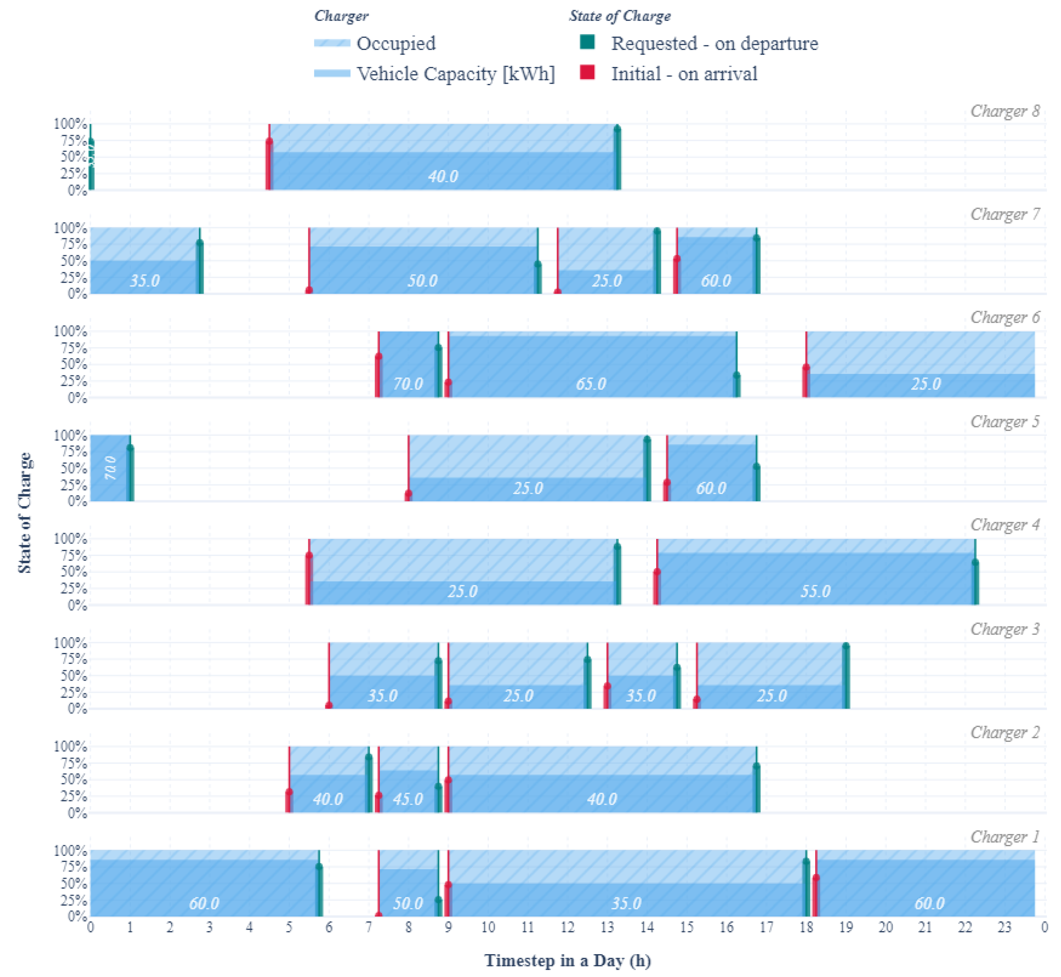
The proposed method is tested on the case study in Croatia. The test case includes EVCS with eight commonly used AC 22 kW chargers considered for possible installation at a rotational parking lot with eight parking spaces. The method is tested on data sampled with a resolution of one representative year. The representative year is a non-leap year with 365 days.

3.1. Data and Parameters

The standard time interval for determining peak power in the Croatian power system is 15 min, so every model variant is run with a 15-min time resolution with accordingly sampled input data.

3.1.1. EVCS Data and Parameters

To model EV energy demand patterns accurately, real measurements from publicly accessible university and business EVCS data were utilized [45,46,47,48]. These measurements have been extensively referenced and validated in prior research by Lee et al. [49], Amara-Ouali et al. [50], Akil et al. [51], and Šolić et al. [52]. By utilizing this data, probability density functions of electric vehicle arrivals/departures and energy requirements were defined. These functions were instrumental in simulating realistic EV charging requests. Figure 4 shows the modelled demand pattern for 19 January. The characteristics that model variants use, as presented in the figure, include a time of arrival or departure, initial vehicle state of charge (SOC) on arrival, requested SOC on departure, charger occupancy period, and vehicle battery capacity. For each EV capacity, the figure displays energy capacity numerically as the value in kWh and visually as a portion of the highest EV battery capacity during this day. As depicted in the Figure 4, most vehicle arrivals happen in the early morning and rarely in the afternoon. Company vehicles have different patterns and usually charge overnight or when unused, as seen in the figure for charger 1 and partly for chargers 5, 6 and 7. Similarly, demand patterns and characteristics are generated for each day throughout a representative year, following the same approach used for 19 January.

There are eight parking lots, each with its own vehicle charger. Investment costs per single parking lot amount to 1000 EUR/lot, while maintenance costs equal only 3% of the investment. EV parameters like (dis)charging efficiency, CC-CV mode switch threshold and charger maximum rated power depend on the EV. However, in this model, it is assumed that they are the same for every EV using EVCS at some time. The building contracted power, as well as parameters for charging stations (CS) and electric vehicles (EV), are specified in

Table 1. Building, CS and EV technical and financial parameters.

Parameter	Unit	Value	Description
$N^{PL}$	–	8	Number of EV chargers/parking lots
${\eta }_{ch}^{EV}$	p.u.	0.95	EV Charging efficiency
${\eta }_{ds}^{EV}$	p.u.	0.95	EV Discharging efficiency
${\alpha }_{threshold}^{CC-CV}$	p.u.	0.9	EV CC-CV mode switch threshold
$P_{max}^{EV}$	kW	22	EV charger maximum rated power
$c_{var}^{PL}$	EUR/lot	1000	Investment variable costs per lot
${\alpha }_{oper}^{PL}$	% investment	3	Parking maintenance cost ratio
$P_{contracted}^{OD}$	kW	150	Building contracted power

.

3.1.2. BESS System Parameters

If the optimization model includes BESS in the EVCS power supply, the financial model includes its costs, considering the battery system’s lifetime of 10 years. The investment costs amount to 200 EUR/kWh, while replacement costs are significantly lower than the investment due to BESS cost decline projections.

Table 2. BESS technical and financial parameters.

BESS System Parameter	Unit	Value	Description
$E_{capacity}^{BES{S}_{max}}$	kWh	1000	Maximum capacity
${\eta }_{ch}^{BESS}$	p.u.	0.95	Charging efficiency
${\eta }_{ds}^{BESS}$	p.u.	0.95	Discharging efficiency
${\alpha }_{DoD}^{BESS}$	p.u.	0.1	Depth of Discharge (DoD)
${\alpha }_{threshold}^{CC-CV}$	p.u.	0.9	CC-CV mode switch threshold
$c_{var}^{BESS}$	EUR/kWh	200	Investment variable costs
${\alpha }_{oper}^{BESS}$	% investment	2	Maintenance cost ratio
$N_{replacement}$	year	10	System replacement year, i.e., system lifetime
${\alpha }_{replacement}^{BESS}$	p.u.	0.3	Replacement cost ratio

shows charging and discharging efficiency, Depth of Discharge and other BESS parameters.

3.1.3. PV System Data

Model variants use existing time series data from an actual PV plant near the potential EVCS location to realistically model the PV system power production. Data are normalized according to the PV plant installed capacity to enable the use of relative solar production data in the proposed optimization method. Figure 5 shows the relative production per time in a day and per day in a year.

Regarding the financial model, investment costs amount to 1500 EUR/kWp, while operational costs equal 2% of total investment costs. Furthermore, the PV system lifetime equals the project lifetime of 25 years, so the optimization model does not consider PV system replacement. The proposed method determines optimal PV system capacity given the top plant limit of 60 kWp based on the system’s potential construction location.

Table 3. PV system technical and financial parameters.

PV System Parameter	Unit	Value	Description
$P_{max}^{PV}$	kW	60	Maximum installable power
$c_{var}^{PV}$	EUR/kW	1500	Investment variable costs
${\alpha }_{oper}^{PV}$	% investment	2	Maintenance cost ratio

presents an overview of all PV system parameters.

3.1.4. Building Load Data and Parameters

Models 3 and 4, in which the EVCS and the building are connected to the grid through the same PoC, employ the modified power demand data from a representative university building. These data help simulate the demand patterns of an office building object more realistically. Figure 6 shows the building demand heatmap for a representative non-leap year. The heatmap shows visible areas of peak demand during the coldest and the hottest days of the year. There are also visible areas with low demand corresponding to the collective vacation period, enabling testing models on different cases that can occur in real life.

To effectively present data and outcomes from various models, the results from a specific representative day of the year, coinciding with the peak building power demand, are displayed. Peak demand appears on the 19th day, i.e., January 19th, and amounts to 118 kW. The heatmap shows it in a dark red color. Contract with a local distribution system operator limits peak demand. If a building uses more power from the grid than the contracted power, that will increase the electricity costs. That is what smart building and V2B models try to prevent. The building’s contracted power is 150 kW (Table 1).

3.1.5. Grid and Tariff Parameters

In Croatia, the Time-of-use (ToU) tariff model is used, in which tariff costs are higher during peak demand hours than during low demand periods. The grid connection costs are incurred as a one-time payment during the initial grid connection and are defined by the annual peak power, while the peak power costs are paid monthly. When surplus energy from the photovoltaic (PV) system is sold back to the grid, it is reimbursed at a slightly reduced rate compared to the standard energy consumption tariff. Details, including this ratio and other tariff and grid parameters, are provided in

Table 4. Time-of-use tariff costs for industrial consumers in Croatia.

Parameter	Unit	Value	Description
$c_{high}^{EE}$	EUR/kWh	0.285854	EPC 1-high tariff
$c_{low}^{EE}$	EUR/kWh	0.16815	EPC 1-low tariff
$c_{high}^{Grid}$	EUR/kWh	0.029199	GUC 2-high tariff
$c_{low}^{Grid}$	EUR/kWh	0.013272	GUC 2-low tariff
$c_{incentive}^{RES}$	EUR/kWh	0.014	RES tax
$c_{peak}^{Grid}$	EUR/kW	5.176	Peak Power Costs-PPC
${\alpha }^{export}$	p.u.	0.8	Exported energy cost ratio
r	%	2	EPC, GUC and PPC annua  increase
$c_{connect}^{Grid}$	EUR/kW	225	Contracted grid connection cost

¹ EPC—energy production costs. ² GUC—grid usage costs.

.

3.1.6. Financial Parameters

As indicated in

Table 5. Project financial parameters.

Parameter	Unit	Value	Description
Y	years	25	Project lifetime
d	%	7	Discount rate
$f/(1-f)$	% investment	30%/70%	Loan/self-financing ratio
k	%	5	Loan interest rate
$N_{loan}$	years	10	Loan payback time

, the project’s duration spans 25 years and is financed in part through a loan, which accounts for only 30% of the overall investments. The repayment of the loan occurs over a ten-year period with an annual interest rate of 5%.

3.2. Workflow

Figure 7 shows the entire process involved in this work. Using Python programming language, input data defined in the previous subsection are loaded and preprocessed according to the required usage. The input data cover the EVCS component, which is also presented in Figure 7. Next, using the Pyomo library, a concrete model is defined based on the algorithm formulations defined in Section 2.2. The concrete model is then used in the model construction. The constructed model is forwarded to the solver program interface alongside the preprocessed input data. For the optimization process, the Gurobi optimization solver is employed, chosen for its leading position in terms of both speed and performance. The optimization process produces results, which are then processed into appropriate model outputs. Model outputs are then analyzed and presented as plot figures, which are used in the Results section.

3.3. Results and Analysis

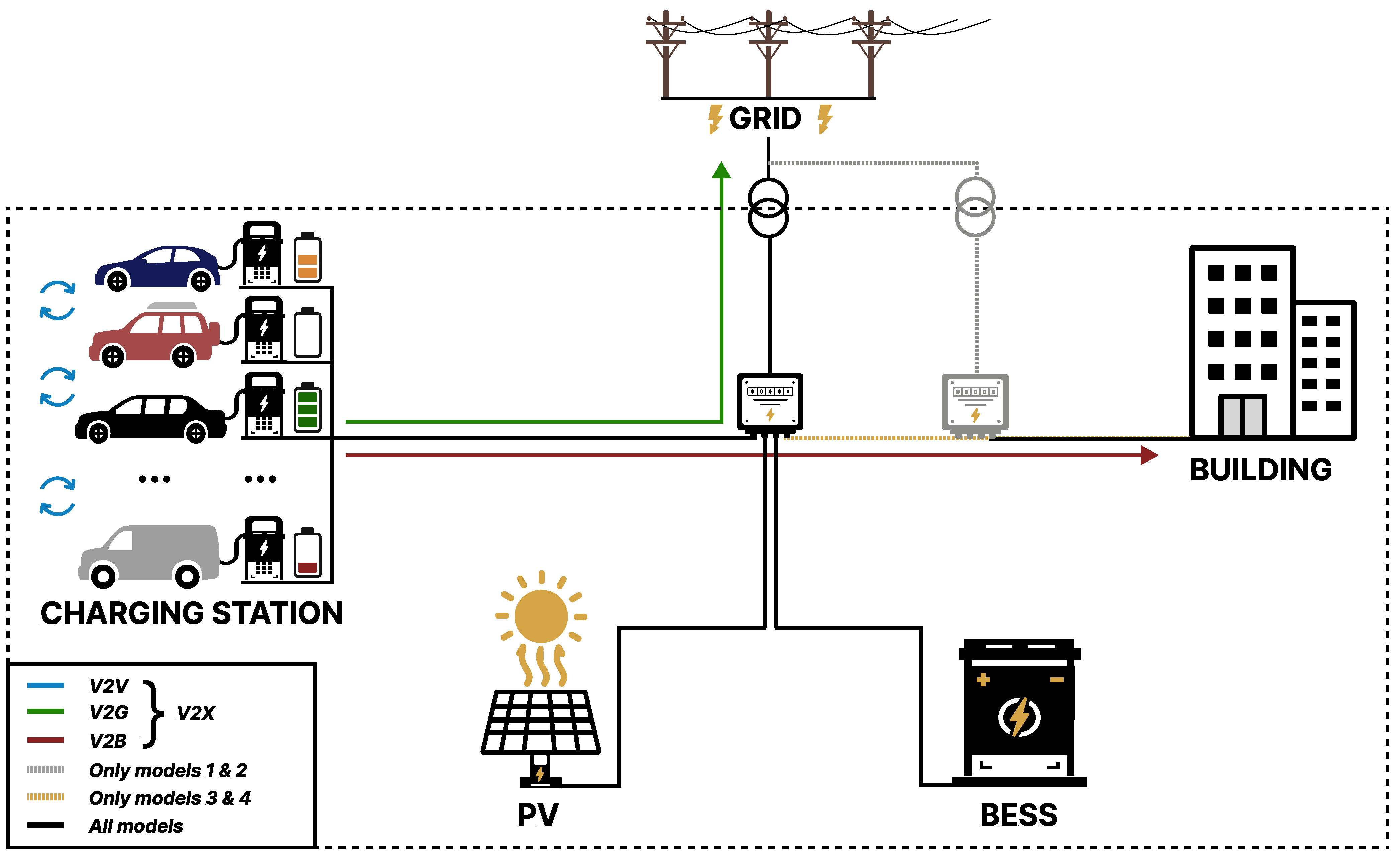
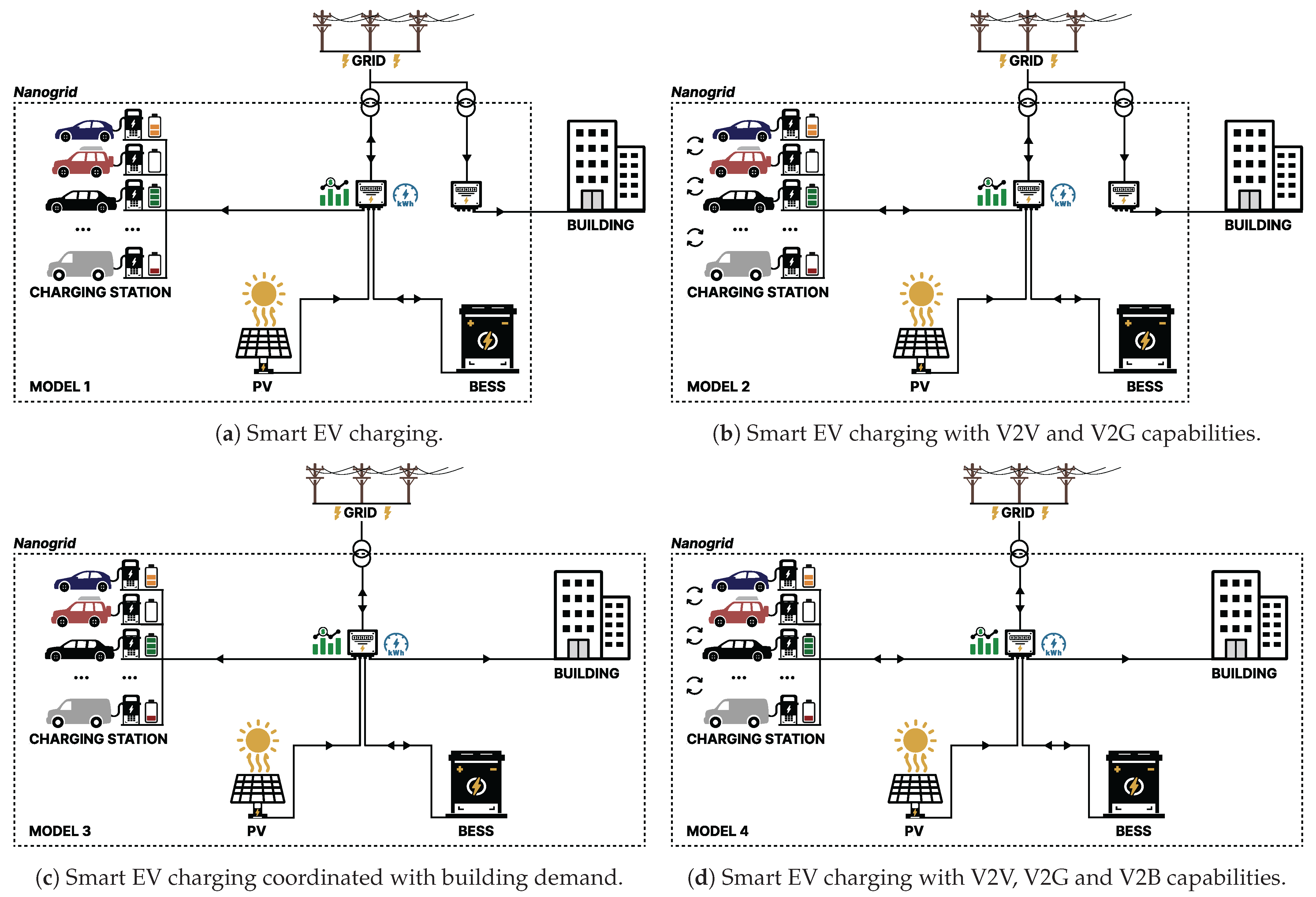
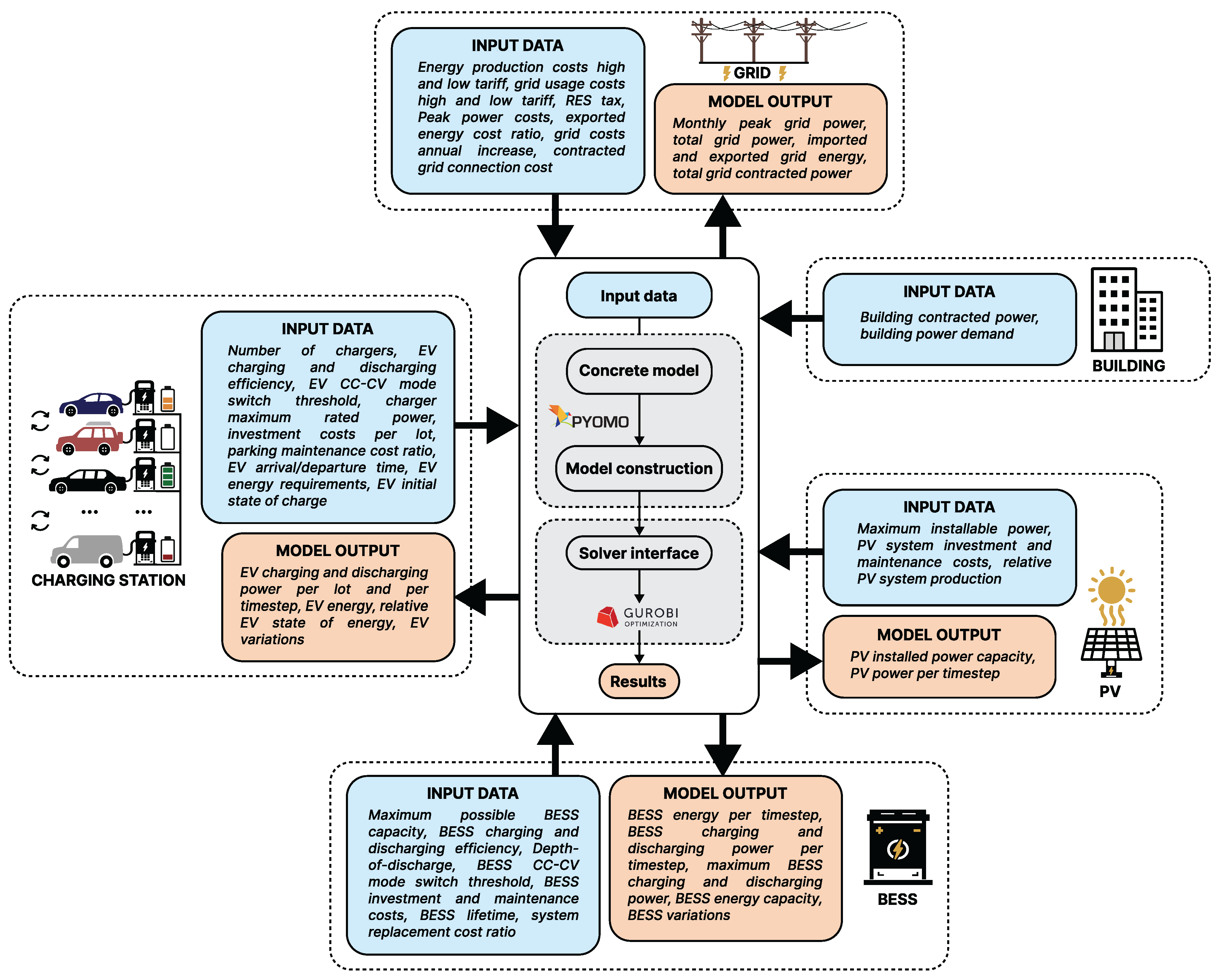
The analysis looks at all EVCS power supply/grid connection variants or separate pairs depending on the common factor, e.g., Models 2 and 4 both include V2X modes, while Models 3 and 4 consider joint EVCS and building connection. With that noted, Model 4 is the most complex variant and includes everything the other three variants have. In the optimization process, each model opts for incorporating both BESS and PV systems. Interestingly, all variants suggest the installation of a PV system with the highest available capacity of 60 kWp. The optimal BESS capacity differs between the variants, as seen in

Table 6. Optimal BESS and PV variables.

Model Variant	${\mathit{P}}_{\mathit{install}}^{\mathit{PV}}$ [kW]	${\mathit{E}}_{\mathit{capacity}}^{\mathit{BESS}}$ [kWh]	${\mathit{P}}_{\mathit{MAX}}^{\mathit{BESS}}$ [kW]
1 (Smart charging)	60.0	40.38	10.1
2 (V2G and V2V)	60.0	24.19	6.0
3 (Building)	60.0	290.37	72.6
4 (V2B, V2G and V2V)	60.0	247.33	61.8

, with each having a different BESS storage capacity and corresponding maximum (dis)charging power. It is noticeable how models tend to increase the PV system capacity, which goes hand in hand with the conclusions by Van Kriekinge et al. [40]. On the other hand, models tend to decrease the BESS capacity, which is probably due to the BESS having, in total, higher costs because of a lifespan that is shorter than the project’s. It is important to note how, in this paper, BESS degradation is not directly included in the formulations but indirectly through BESS replacement every ten years.

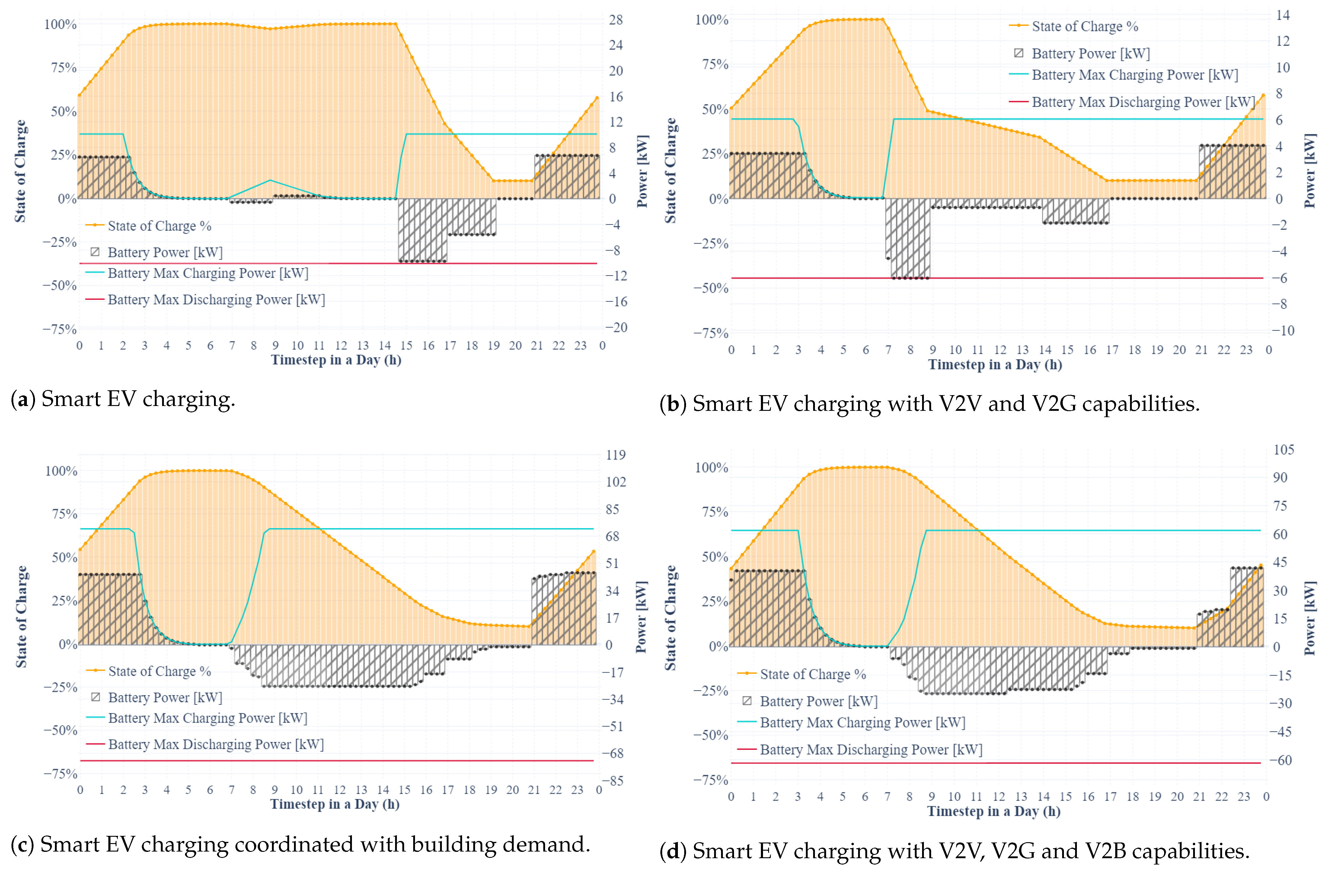
When a model incorporates V2G, V2B, or V2V functionalities, it becomes apparent that the BESS capacity is reduced compared to a scenario involving solely smart charging, aligning with the findings presented by Kucevic et al. [27]. The same also applies to the maximum battery power for charging and discharging. Figure 8 shows this for the representative day in a year for each of the microgrid variants studied in this paper.

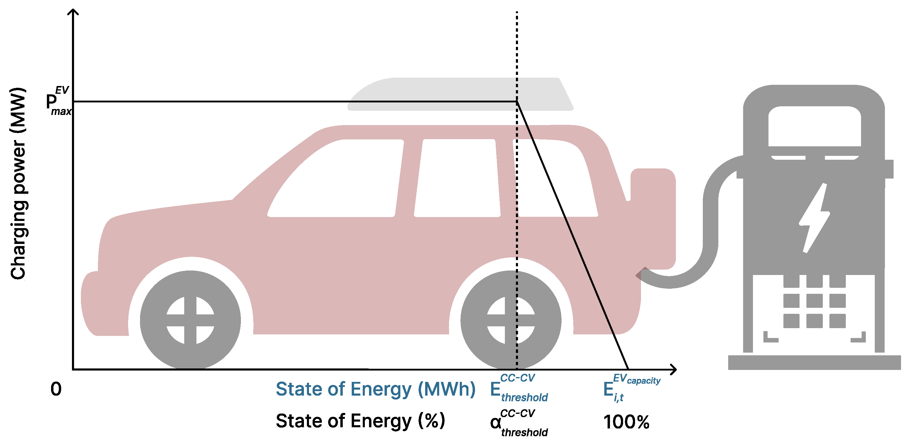
The blue line in Figure 8 represents the maximum charging power, which varies depending on the CC-CV mode constraint, and the red line represents the maximum discharging power. While the red lines are constant, the CC-CV blue line depends on the BESS SOC, with the power decreasing as the SOC comes closer to 100%, and the power increasing as the SOC decreases. The maximum powers in each subplot correspond to the values in Table 6. All four variants charge the BESS at night and use it during the day, i.e., during the time of day with peak tariffs, with variant 1 using it when most vehicles leave (around 3–7 p.m.). Models 3 and 4, which include the building in the microgrid optimization, have a more evenly BESS discharging process than Models 1 and 2. Considering the SOC, the state never reaches below the DoD, and for every model, BESS reaches 100% right before the bulk of vehicles connect to the CS, which is around 5–8 a.m. Most of the time, this happens throughout the representative year as shown in Figure 9. Occasionally, certain days deviate from this typical pattern, especially in models without buildings. These deviations involve either shifting the daily trend or maintaining a relatively consistent SOC throughout the entire day. 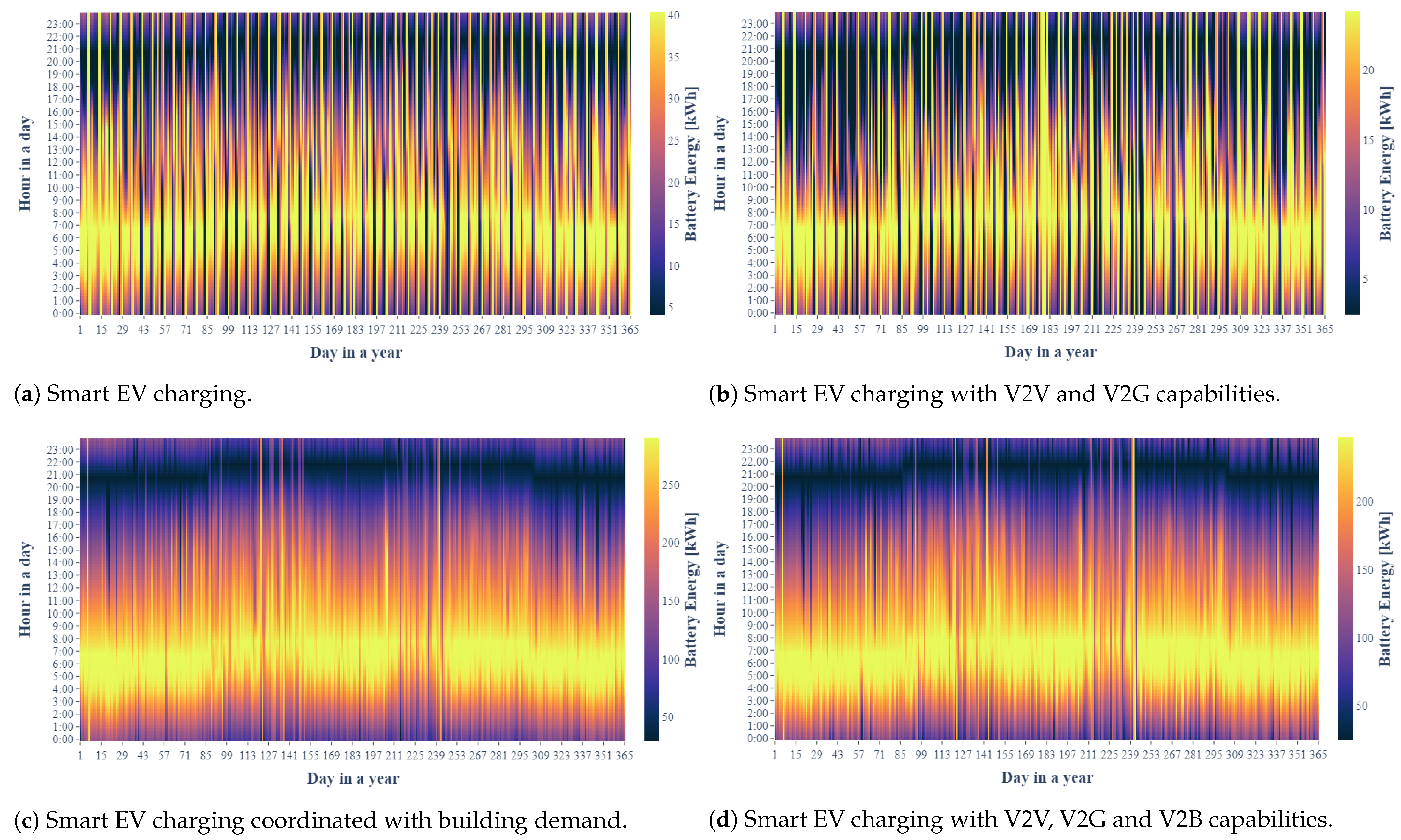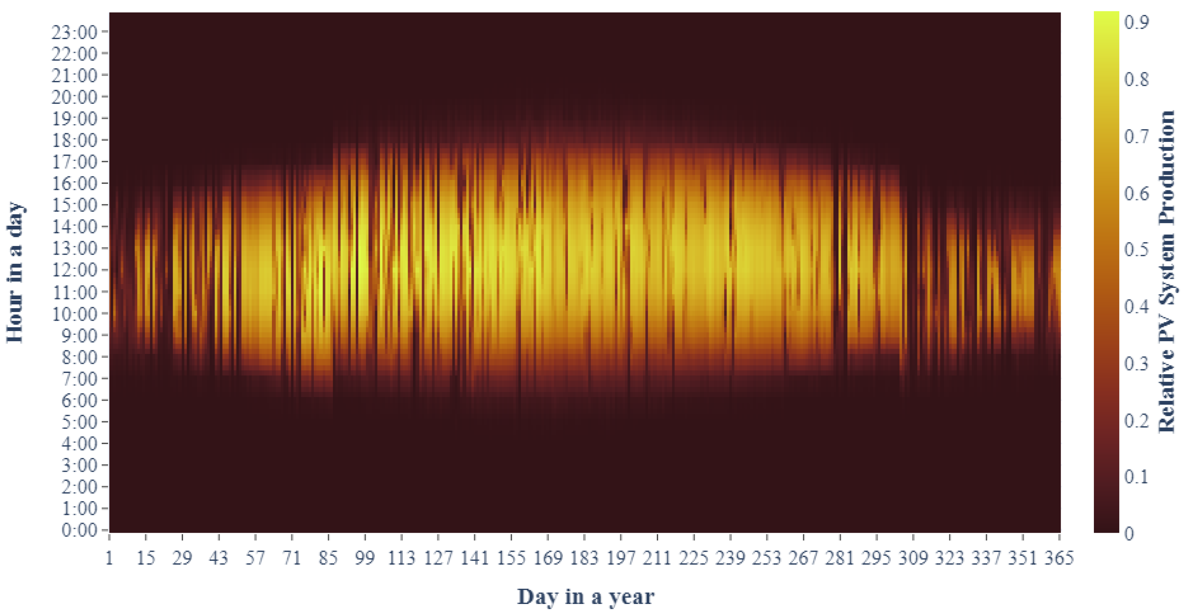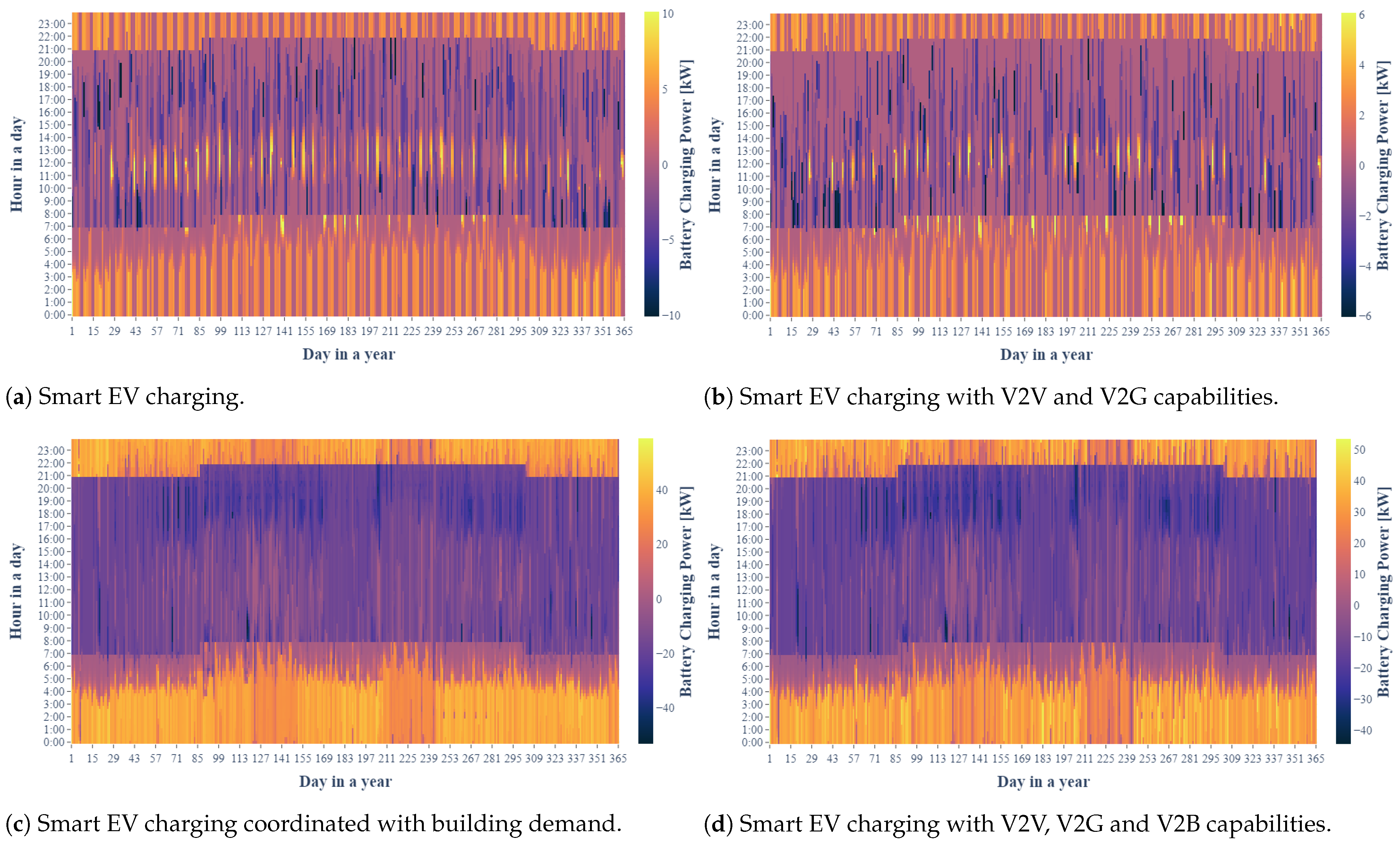Furthermore, Figure 10 broadens the insight into the overall charging trend of BESSs.

Figure 10 shows BESS charging and discharging power during a single representative year. The discharging process mainly happens between 07:00 h and 22:00 h, with the starting and ending times shifting during the middle of the year due to advancing clocks (and high-tariff active periods) for daylight savings time (or summer time) and falling back to the standard time for the rest of the year. During the night and early morning, the BESS usually charges itself. The exceptions are days with larger solar production than consumption, which mostly happens only for Models 1 and 2 and can be seen in the figure as the bright yellow marks during the middle of the day.

Regarding the V2X methods, they minimally affect the BESS system operation. This is evident from the almost identical plots for Models 1 and 2 as well as Models 3 and 4, indicating minor differences, except for the reduced power in the model variants with V2X capability.

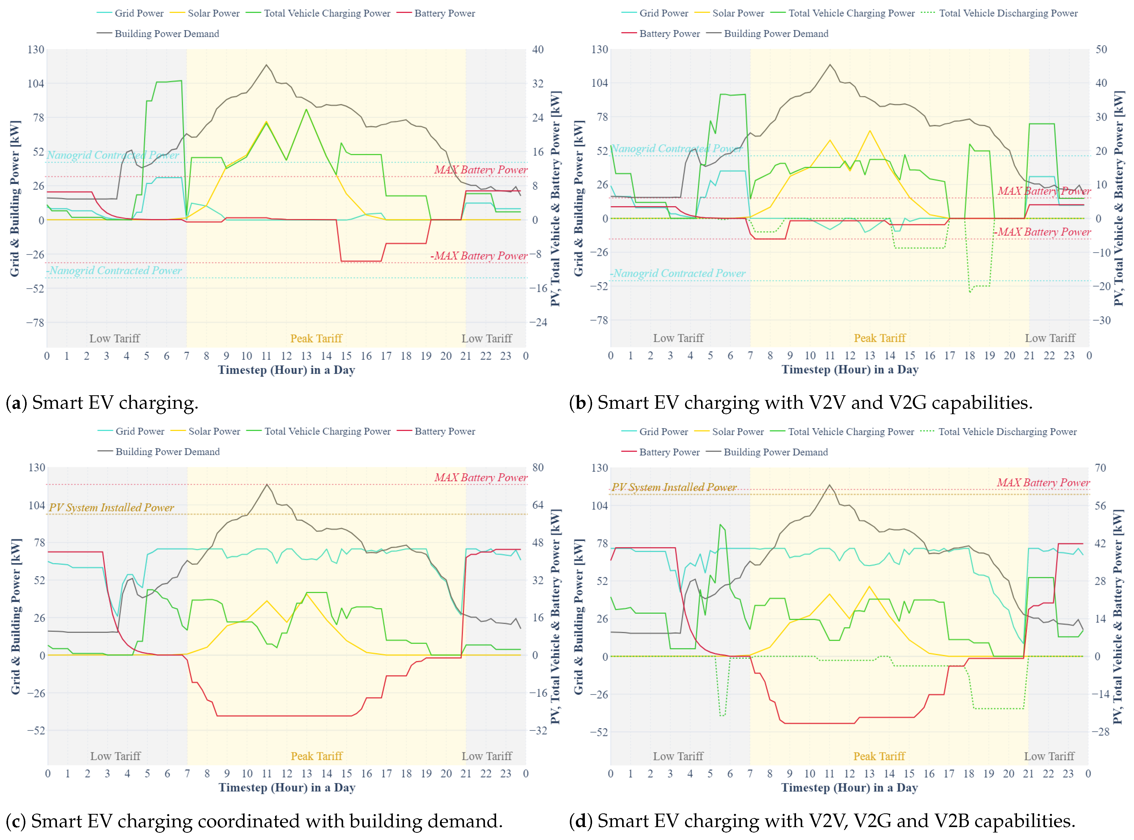
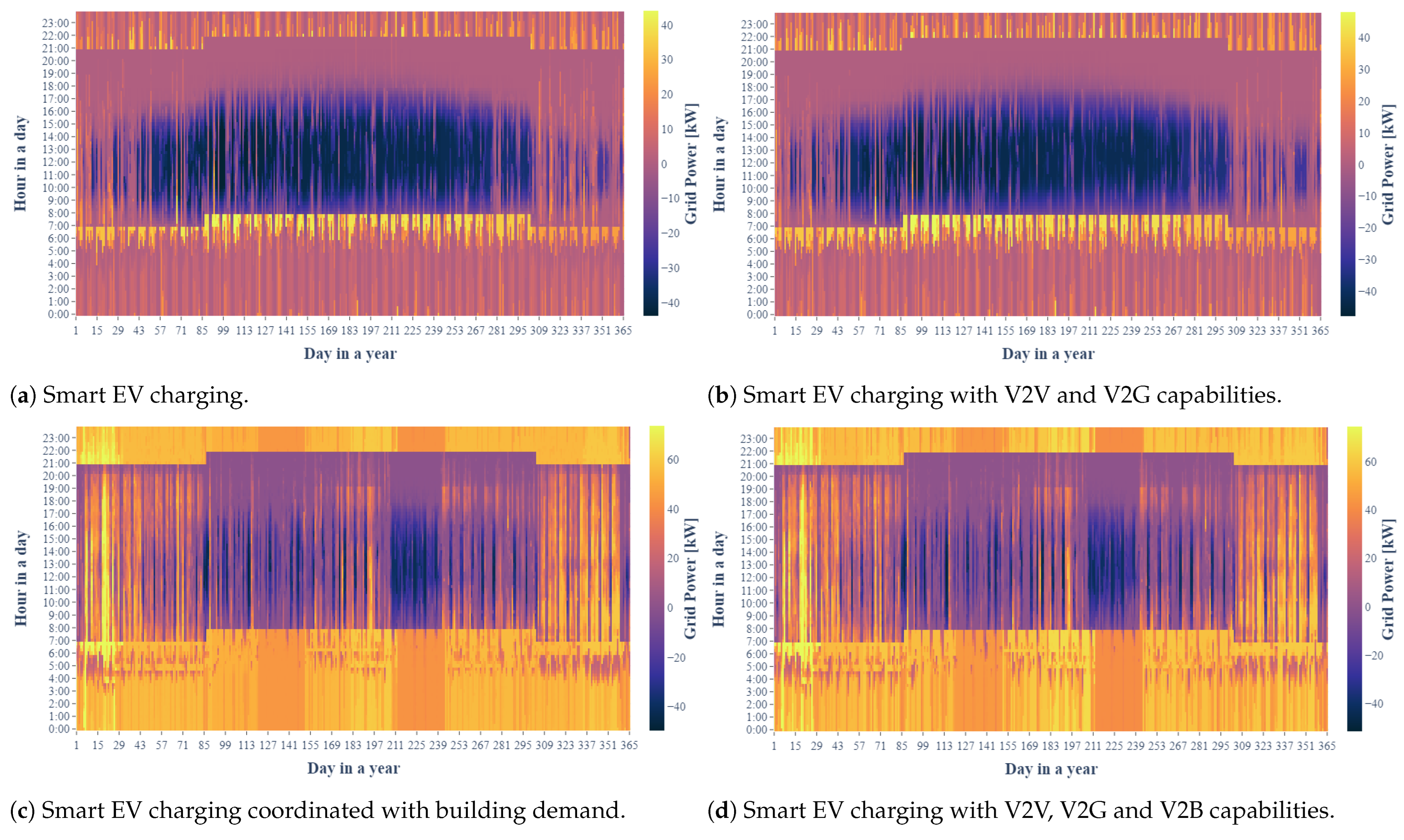
Figure 11 likewise shows the BESS power differences between the models, alongside the visualization of all other power inputs and outputs constituting the power equilibrium in the microgrid. The figure also has marked periods of low and peak tariffs, corresponding to Croatia’s grid tariff and the main office hours of the university or business building. As Figure 11 confirms, the BESS charges mainly during the night from the grid, and its power is used to charge EVs (every model) or to lower the building demand (models 3 and 4) during the peak tariff period. Considering solar power, variants 1 and 2 use it for charging EVs or selling excess power to the grid for profit in cases of excess production, while Models 3 and 4 use it to charge EVs and supply building demand. Models 2 and 4 with V2X capabilities also apply V2V and V2B methods (green dotted line) to either charge leaving or suddenly departing vehicles, or respond to the building demand by lowering grid power import amount and, consequently, the grid cost. This also achieves greater utilization of CS, i.e., when EVs would usually stay idle, they are used for helping the microgrid as manageable loads. Model variants 3 and 4 also have a more even grid power distribution because of the constantly available building demand and BESS operation to minimize the total peak power of both building and EVCS. Models 1 and 2 do not follow that behavior, as they have higher grid demand right before and after the peak tariff period, while during it, it is very low, given that EV charging is coordinated with the PV production. EV charging from the grid during the low-tariff period and from the BESS, PV system and the grid during the peak demand period, as well as discharging some of them to lower the building demand in Models 3 and 4, helps to reduce the peak grid power. This, however, does not achieve net or nearly zero-energy building as in the work of Nazari et al. [35]. To reach that goal, larger solar production or other renewables would be needed, which depends on the area available for the construction of a PV plant or other RES of the required capacity.

As depicted in Figure 11, the V2X operation mode is typically employed prior to the activation of a low-energy tariff. This mode is initiated by EVs departing from EVCS sometime after the low-energy tariff has been activated. During periods of high-energy tariffs, EVs are usually discharged just after high-tariff activation. This process is triggered by EVs that were previously charged during periods of low energy costs and still have ample charging time left, enabling them to recharge using solar energy from photovoltaic (PV) plants.

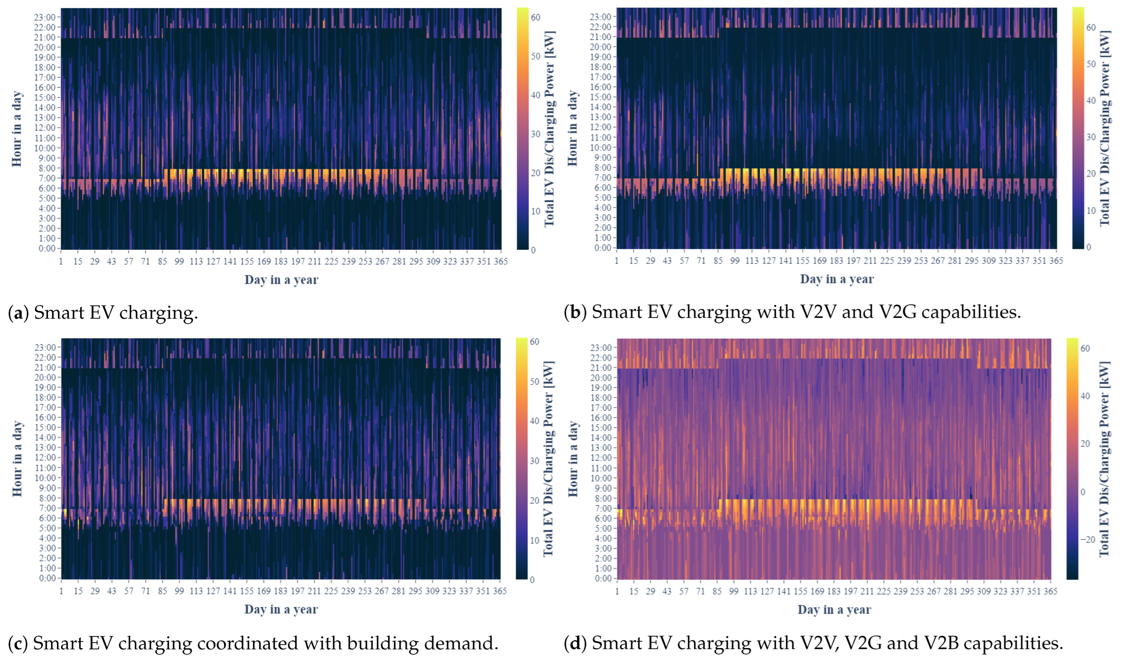
If comparing models with the V2X approach, only model 4 shows negative, i.e., discharging values. There are two reasons for this. Firstly, model 2 mostly applies the V2V method to decrease costs, achieve profit and charge departing vehicles, which is why charging overpowers and nullifies the discharging power in total. Secondly, Model 4, besides using V2V for cases like in Model 2, also applies the V2B method to lower the building’s grid demand effectively, so all rarely occurring discharging events in Figure 12d represent the application of V2B. That is also why models with V2X have, at a glance, fewer charging events than models without it. For this use case, it is important to note how vehicle demand patterns are applied for a higher per-charger utilization rate due to the current small percentage of EV owners in Croatia, and consequently, these results represent EV charging characteristics in the future or near future scenario. Figure 13 illustrates the total power imported and exported to the grid throughout the representative year.

Imports and exports to the grid in Figure 13 reveal key patterns within the microgrid for different operating models. It is possible to see the peak grid power demand occur during January. Moreover, the PV system’s patterns are observable, mainly because only excess solar power can be sold to the grid for profit. In Models 3 and 4, this only happens during the period with low building demand during the spring with mild temperatures or during August when, for this use case, most employees are on their collective annual summer vacation. The same spring and summer pattern can also be seen in Figure 10 and Figure 12.

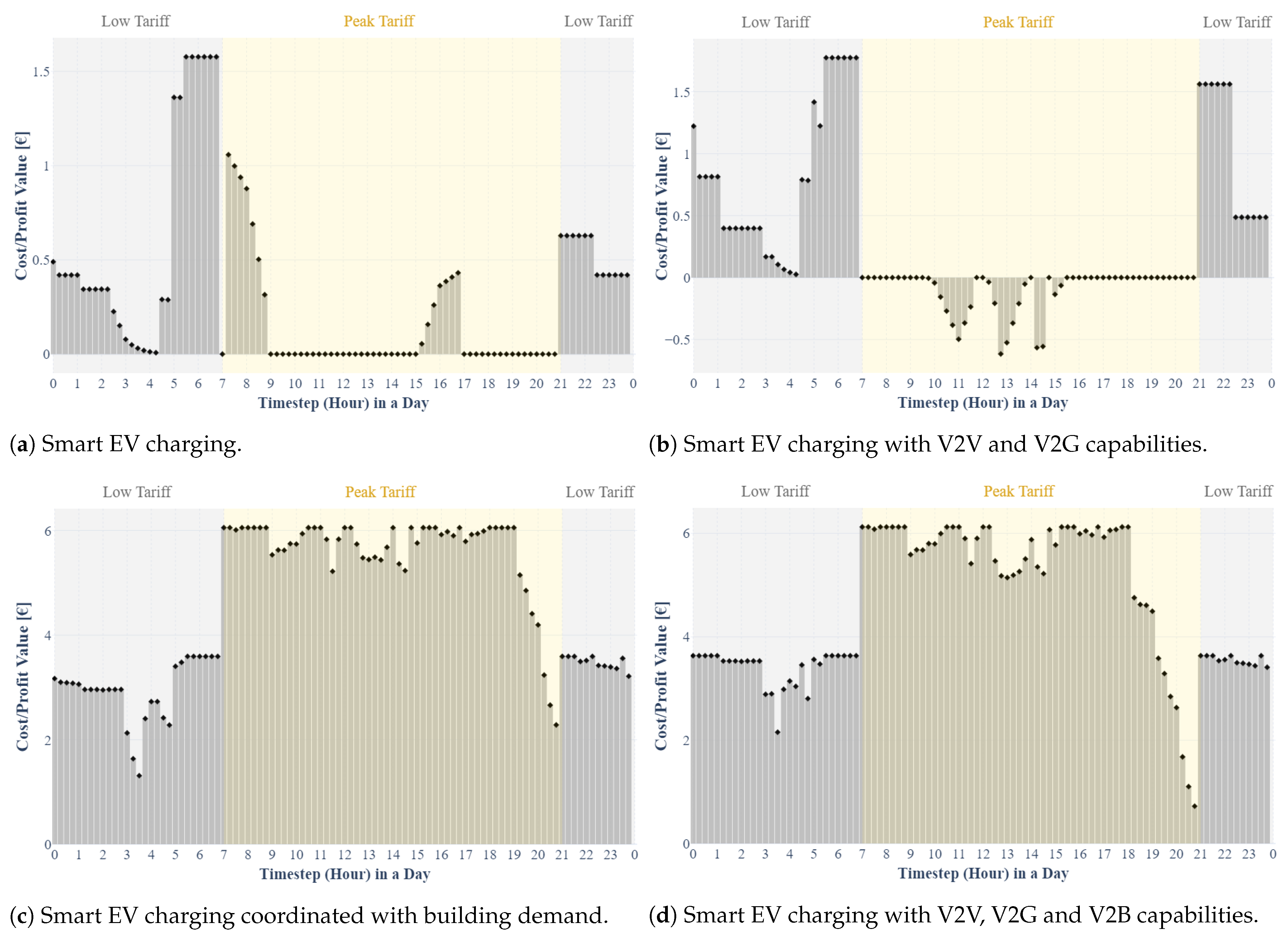
Figure 14 shows the optimized resulting costs for the representative day for each 15 min interval. Models 1 and 2 only show the CS costs, excluding the building costs, which increase the daily expenses. With that in mind, it is observable that, considering the CS, the most significant part of the costs for variants 1 and 2 occur during the low-tariff period, while for Models 3 and 4, the highest costs are reached during the day due to the building having its highest power demand during that time. It can also be seen that daily costs for models with implemented V2X methodology do not differ significantly from those without it.

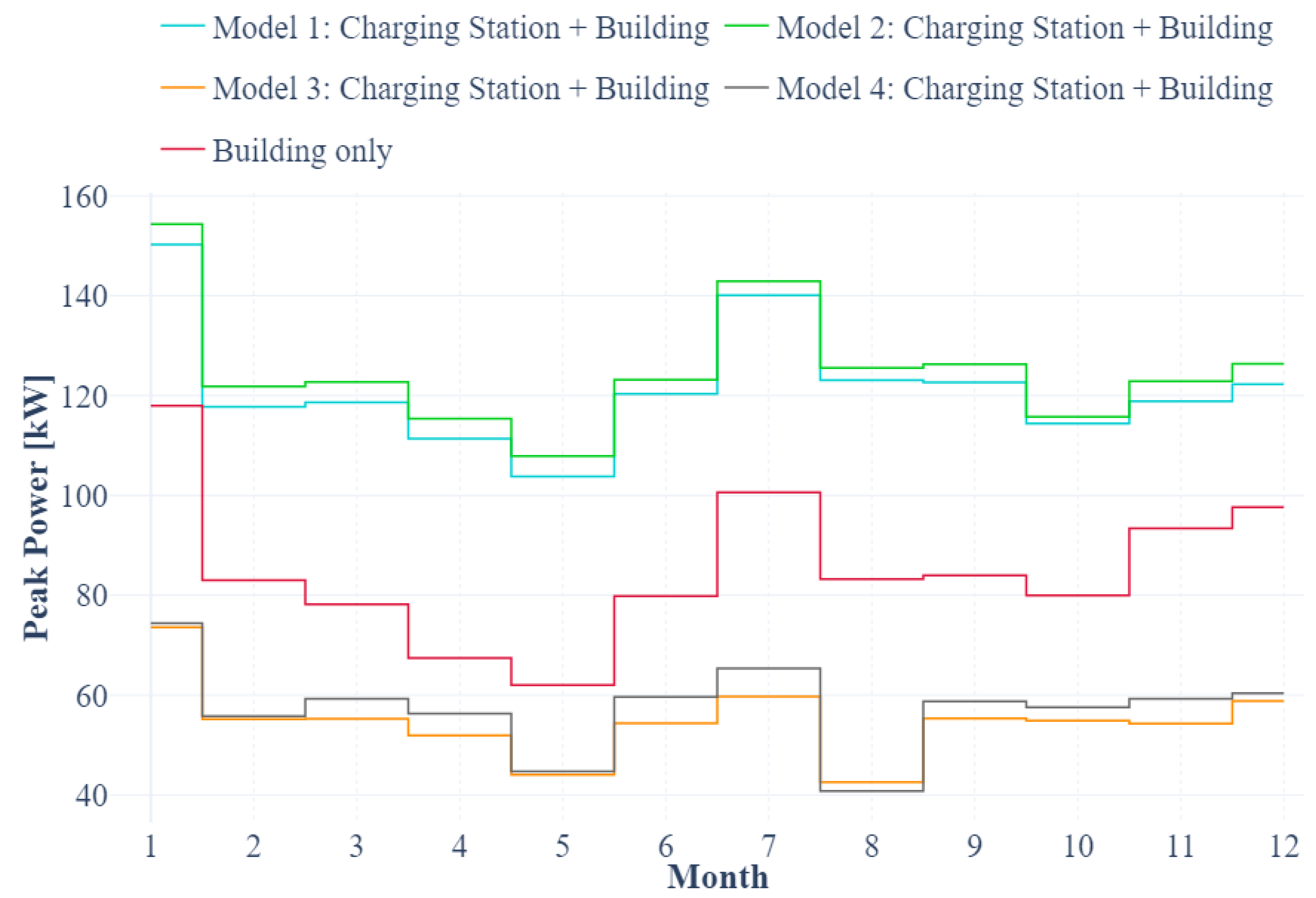
The same is true for the monthly peak grid powers (Figure 15) and the total costs (Figure 16). Examining the monthly peak powers per model, it is evident that Models 3 and 4, incorporating both a building and the charging station in the optimization model, outperform the building on its own in terms of monthly peak power. Models 1 and 2 are suboptimal because they involve independent management of the EVCS and the building, focusing solely on optimizing the EVCS peak power costs without incorporating them into the building’s existing power demand. Managing and optimizing EVCS together with the building leads to an average decrease in the monthly peak power by around 34% regarding the building itself, while separate managing leads to an increase by around 44%. Moreover, the monthly peak powers and associated costs for Models 1 and 2 are approximately twice greater than for Models 3 and 4.

While the models employing V2X methodology exhibit higher peak powers compared to those without it, as indicated in Figure 15, the opposite holds true for total costs. The slight increase in peak power in models incorporating V2X operation is attributed to the lower optimal BESS capacity determined by the model. This reduced BESS capacity limits the microgrid operational flexibility and the potential for reducing peak power.

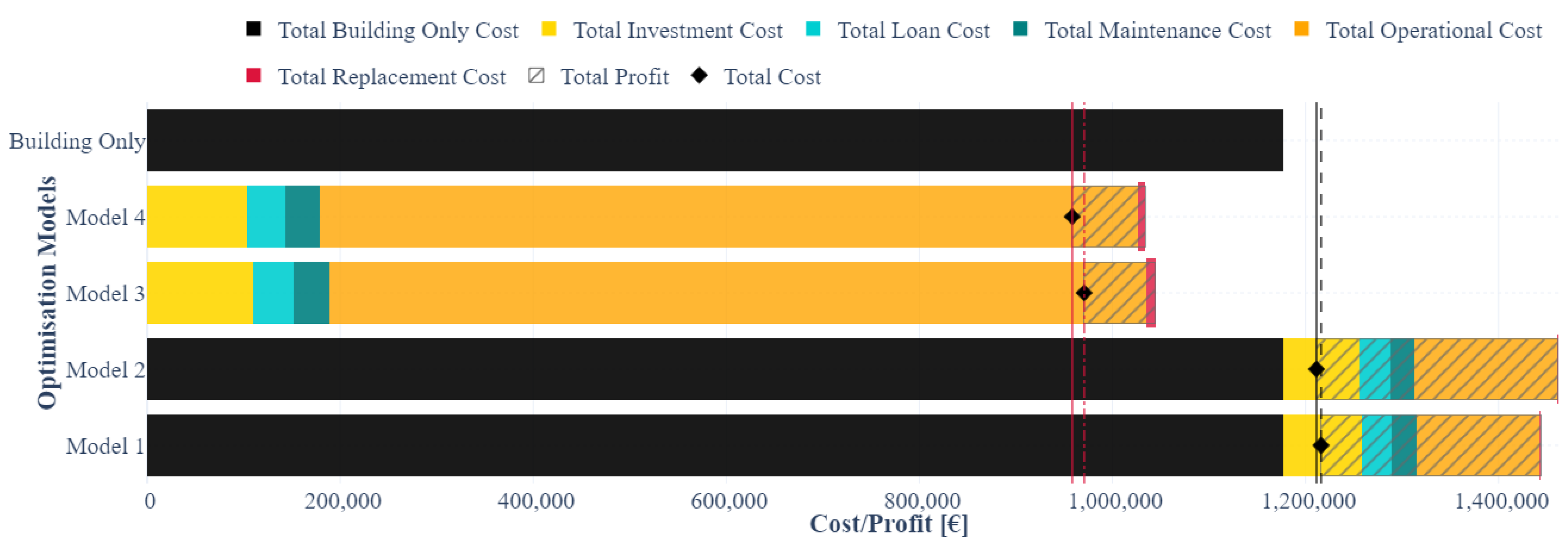
Figure 16 gives an overview of the main cost components contributing to the net present cost of the entire project over its 25-year lifespan.

It is evident that in Models 3 and 4, the costs within each category are higher, mainly because these models include building energy costs in the optimization model. Nevertheless, the overall total costs in models 3 and 4 still outperform those in models 1 and 2, as well as the building energy costs when operating separately from EVCS. The primary factor behind the substantial cost reduction in Models 3 and 4 is the direct utilization of PV energy to supply EVCS but also building demand, thereby reducing the excess energy exported to the grid at lower selling prices (in relation to load supply prices). While incorporating V2X operation does contribute to overall cost reduction, its impact is not as significant.

Comparing the models with V2X and those without it, V2X contributes to the higher profit, which ensures more considerable savings for the microgrid using V2X methodologies. Model 4 with V2B, V2G and V2V is in every aspect better than Model 3. Model 2 has greater operational costs than Model 1, but due to the larger profit, its total cost is lower than that of Model 1, where the larger profit is a consequence of employing V2G and V2V, allowing the sale of excess solar production during the day directly to the grid. Lower investment, loan, maintenance and replacement costs in models with the V2X approach result from the smaller BESS capacity selected in the optimization process. With all that information in mind, the most optimal smart microgrid model is Model 4, the most complex model of all variants considered in this paper.

Table 7. Total costs and cost difference per model variant.

Model Variant	Total Cost [EUR]	Cost Increase or Decrease in Comparison with Building Only Cost [EUR] 1	Cost Difference between Models Paired Considering with and without Building Included (1 vs. 3; 2 vs. 4) [EUR] 2
1	1.216.199	39.350	245.358
2 (V2G and V2V)	1.211.409	34.560	253.022
3 (With building)	970.840	−206.008	−245.358
4 (V2B, V2G and V2V)	958.387	−218.461	−253.022
Only building (no CS)	1.176.849	–	–

¹ Positive values—cost increase; negative values—cost decrease. ² Positive values: model 1-model 3, model 2-model 4; negative values: model 3-model 1, model 4-model 2.

shows the total costs per model for a more detailed comparison and insight into the exact cost differences amount.

It is evident from Figure 11, Figure 13, Figure 14, Figure 15 and Figure 16 how large-scale services cannot generate any, or at least any significant, revenues from direct energy trade, just as Borghetti et al. [32] claim. However, it is clear that applying this approach, specifically Models 3 and 4, achieves significant savings in the long run, similar to Aparicio and Grijalva [37]. To generate additional profit in cases when it is applicable and appropriate, a fee can be imposed, whether on charging EVs themselves or on a parking service, like Moura et al. propose in [43,44], depending on the circumstances.

Regarding the influence of V2X methodologies on the total cost, it is important to note that even though this work determines optimal EVCS (dis)charging management, the main goal of the model is to optimally dimension potential power sources and to estimate the EV charging cost with optimal EVCS mode of operation for the total of the project’s lifetime considering both investment and operational costs, which can be seen in Table 7. Therefore, the algorithm does not explicitly consider all stochastic scenarios, e.g., the sudden departure of one or more EVs from the EVCS. Those scenarios are rather indirectly modeled into the simulation by using real data from existing EVCS in the arrival/departure scenario generating process. Because of that, in the mentioned scenarios, depending on the selected power supply method, the model independently determines in which way to satisfy the user’s charging request in that short period of time. The model itself determines the (dis)charging strategy to implement in a given situation, depending on the possibilities and the general impact of each action on the total costs. An example of such an action, implementing V2X, can be seen in Figure 11b model 2, which is not influenced by building demand, where at the end of the working day, when most vehicles are departing, the charging and discharging of EVs simultaneously occur. Generally, the possibilities of meeting the requests of users who, unannounced, stop the charging operations are limited due to the limited time and power constraints. Furthermore, it is also questionable whether there is an obligation to comply with the request of the user who suddenly changes the initial charging requests. In this case, it is rather difficult to achieve. This is difficult to achieve even in the case of a per-day-basis EVCS and EV-charging management, but in that case, it would be possible if EVs frequently visit the EVCS and, therefore, if modeling the data includes identification information about particular EVs. That, however, is not the focus of this work and would require a different and more complex approach.

4. Conclusions

In summary, this study presents an innovative method employing mixed-integer linear programming formulation, aiming to achieve three key goals. These goals include optimizing charging schedules and power supply strategies for EVCSs while integrating seamlessly with existing building demand. Additionally, the approach focuses on minimizing the net present value of both the capital investment and operational costs of EVCS. The study also assesses the impact of smart charging, V2X techniques, and grid connection alternatives, aiming to reduce overall charging costs effectively.

The study compares four model variants, some employing smart charging alone and others integrating V2X methods. Additionally, the presence or absence of a building within the microgrid context is explored. The results reveal that models that consider a joint grid connection of EVCS and building, despite having higher costs within individual categories due to the inclusion of building energy expenses, demonstrate superior performance in terms of overall total costs over the project’s lifespan. This cost reduction is primarily attributed to joint power supply optimization and the direct utilization of PV energy for both EVCS and building demand, minimizing excess energy exports to the grid at lower prices. Furthermore, while the incorporation of V2X operations does contribute to cost reduction, its impact is comparatively modest. The total cost reduction will also be influenced by incentives that end consumers receive for participating in such operations but also by operational costs related to the management and maintenance of the V2B, V2V and V2G charging infrastructure. This suggests that the direct integration of renewable energy sources, particularly PVs, plays a pivotal role in achieving significant cost savings and EV charging cost reduction. Given that the V2G option in combination with the optimal BESS offers the potential for providing ancillary services and the generation of extra income, future research will focus on extending the proposed model to include these aspects in the EVCS power supply optimization problem. Additionally, understanding the intricate balance between EV consumer incentives and operational costs in V2B, V2V, and V2G charging strategies is crucial. In this sense, future research will also focus on determining the levelized cost of EV charging for different charging strategies as well as on policy recommendations that stimulate EV participation.

In conclusion, this research not only sheds light on optimal charging strategies and power supply methods for EVCS but also emphasizes the critical importance of integrating renewable energy sources efficiently. By leveraging renewable energy directly for both building and EVCS needs, substantial reductions in overall project costs can be achieved, paving the way for a more sustainable and economically viable electric vehicle infrastructure with reduced grid impact.

References

1. Infographic-Fit for 55: Why the EU is Toughening CO2 Emission Standards for Cars and Vans. Available online: https://www.consilium.europa.eu/en/infographics/fit-for-55-emissions-cars-and-vans/ (accessed on 12 September 2022).
2. Here’s How EU Legislation Accelerates the EV Revolution. Available online: https://www.virta.global/blog/this-is-how-eu-regulation-accelerates-the-electric-vehicle-revolution (accessed on 12 September 2022).
3. New Registrations of Electric Vehicles in Europe. Available online: https://www.eea.europa.eu/ims/new-registrations-of-electric-vehicles#footnote-3URSKG9P (accessed on 12 September 2022).
4. Electric Vehicle Outlook 2022. Available online: https://bnef.turtl.co/story/evo-2022/page/1?teaser=yes (accessed on 26 September 2022).
5. Energy Monitor: Have Booming EV Sales Crossed the Mass-Adoption Tipping Point? Available online: https://www.energymonitor.ai/sectors/automotive/electric-vehicle-tipping-point (accessed on 23 September 2022).
6. Electrek: This Is Where Electric Vehicle Adoption Is Headed between 2022 and 2025. Available online: https://electrek.co/2022/05/31/this-is-where-electric-vehicle-adoption-is-headed-between-now-and-2025/ (accessed on 26 September 2022).
7. Treehugger: Will EV Costs Go Down? Understanding the Future of Electric Car Prices. Available online: https://www.treehugger.com/will-ev-costs-go-down-5200295 (accessed on 26 September 2022).
8. Barriers to Electric Vehicle Adoption in 2022. Available online: https://www.exro.com/industry-insights/barriers-to-electric-vehicle-adoption-in-2022 (accessed on 26 September 2022).
9. The Verge: EV Prices Are Going in the Wrong Direction. Available online: https://www.theverge.com/2022/8/24/23319794/ev-price-increase-used-cars-analysis-iseecars (accessed on 23 September 2022).
10. Electric Car Prices and Uncertainty about Charging Availability Remain the Biggest Obstacles to EV Adoption in Europe. Available online: https://news.evbox.com/en-WW/213975-electric-car-prices-and-uncertainty-about-charging-availability-remain-the-biggest-obstacles-to-ev-adoption-in-europe (accessed on 26 September 2022).
11. EVBox Mobility Monitor 2022. Available online: https://evbox.com/en/mobility-monitor-2022 (accessed on 26 September 2022).
12. Treehugger: Will Lithium Prices Kill Demand for Electric Cars? Available online: https://www.treehugger.com/will-lithium-prices-kill-demand-for-evs-5223980 (accessed on 26 September 2022).
13. Our World in Data: The Price of Batteries Has Declined by 97% in the Last Three Decades. Available online: https://ourworldindata.org/battery-price-decline (accessed on 26 September 2022).
14. Green Car Reports: EV Affordability Threatened by Cobalt Prices: Did the US Let Resource Control Lapse over Oil? Available online: https://www.greencarreports.com/news/1135424_ev-affordability-threatened-by-cobalt-prices-did-the-us-let-resource-control-lapse-over-oil (accessed on 26 September 2022).
15. EV Battery Technology: The Road to a Breakthrough. Available online: https://www.investors.com/news/ev-battery-technology-hunting-for-the-next-big-thing (accessed on 26 September 2022).
16. Three Battery Technologies That Could Power the Future. Available online: https://www.saftbatteries.com/media-resources/our-stories/three-battery-technologies-could-power-future (accessed on 26 September 2022).
17. New York Times: Carmakers Race to Control Next-Generation Battery Technology. Available online: https://www.nytimes.com/2022/03/07/business/energy-environment/next-generation-auto-battery.html (accessed on 26 September 2022).
18. Future Batteries, Coming Soon: Charge in Seconds, Last Months and Power over the Air. Available online: https://www.pocket-lint.com/gadgets/news/130380-future-batteries-coming-soon-charge-in-seconds-last-months-and-power-over-the-air (accessed on 26 September 2022).
19. Smart, J.G.; Salisbury, S.D. Plugged In: How Americans Charge Their Electric Vehicles; Idaho National Laboratory (INL): Idaho Falls, ID, USA, 2015; p. 3. [Google Scholar]
20. Electric Vehicles and the Charging Infrastructure: A New Mindset? Available online: https://www.pwc.com/us/en/industries/industrial-products/library/electric-vehicles-charging-infrastructure.html#content-free-1-2e82 (accessed on 26 September 2022).
21. The National Renewable Energy Laboratory (NREL): Documenting a Decade of Cost Declines for PV Systems. Available online: https://www.nrel.gov/news/program/2021/documenting-a-decade-of-cost-declines-for-pv-systems.html (accessed on 23 November 2022).
22. Reshmi, K.M.; Divya, N.A. Cost Analysis of a Smart Home Energy Management System-A Case Study. In Proceedings of the 2022 IEEE International Conference on Signal Processing, Informatics, Communication and Energy Systems (SPICES), Thiruvananthapuram, India, 10–12 March 2022; pp. 366–371. [Google Scholar] [CrossRef]
23. Kannan, D. Time-of-Use Tariff and Valley-Filling Based Scheduling Algorithm for Electric Vehicle Charging. Master’s Thesis, University of Stuttgart, Stuttgart, Germany, 6 April 2021. [Google Scholar]
24. CIRED Work Group 2018–1. In Load Modelling and Distribution Planning in the Era of Electric Mobility. In Proceedings of the International Conference on Electricity Distribution (CIRED), Liège, Belgium, 20–23 September 2021; pp. 21–53. [Google Scholar]
25. Dukpa, A.; Butrylo, B. MILP-Based Profit Maximization of Electric Vehicle Charging Station Based on Solar and EV Arrival Forecasts. Energies 2022, 15, 5760. [Google Scholar] [CrossRef]
26. Li, Y.; Li, K. Incorporating Demand Response of Electric Vehicles in Scheduling of Isolated Microgrids With Renewables Using a Bi-Level Programming Approach. IEEE Access 2019, 7, 116256–116266. [Google Scholar] [CrossRef]
27. Kucevic, D.; Göschl, S.; Röpcke, T.; Hesse, H.; Jossen, A. Reducing grid peak load through smart charging strategies and battery energy storage systems. In Proceedings of the 5th E-Mobility Power System Integration Symposium (EMOB 2021), Berlin, Germany, 27 September 2021; pp. 210–213. [Google Scholar] [CrossRef]
28. Mignoni, N.; Carli, R.; Dotoli, M. Distributed Noncooperative MPC for Energy Scheduling of Charging and Trading Electric Vehicles in Energy Communities. IEEE Trans. Control. Syst. Technol. 2023, 31, 2159–2172. [Google Scholar] [CrossRef]
29. Tushar, M.H.K.; Zeineddine, A.W.; Assi, C. Demand-Side Management by Regulating Charging and Discharging of the EV, ESS, and Utilizing Renewable Energy. IEEE Trans. Ind. Inform. 2018, 14, 117–126. [Google Scholar] [CrossRef]
30. O’Malley, C.; Aunedi, M.; Teng, F.; Strbac, G. Value of Fleet Vehicle to Grid in Providing Transmission System Operator Services. In Proceedings of the 2020 Fifteenth International Conference on Ecological Vehicles and Renewable Energies (EVER), Monte-Carlo, Monaco, 10–12 September 2020; pp. 1–8. [Google Scholar] [CrossRef]
31. Meenakumar, P.; Aunedi, M.; Strbac, G. Optimal Business Case for Provision of Grid Services through EVs with V2G Capabilities. In Proceedings of the 2020 Fifteenth International Conference on Ecological Vehicles and Renewable Energies (EVER), Monte-Carlo, Monaco, 10–12 September 2020; pp. 1–10. [Google Scholar] [CrossRef]
32. Borghetti, F.; Colombo, C.G.; Longo, M.; Mazzoncini, R.; Panarese, A.; Somaschini, C. Vehicle-To-Grid: A Case Study of ATM E-Bus Depots in the City of Milan in Italy. In Proceedings of the 2021 AEIT International Annual Conference (AEIT), Milan, Italy, 4–8 October 2021; pp. 1–6. [Google Scholar] [CrossRef]
33. Maigha, M.; Crow, M.L. A Transactive Operating Model for Smart Airport Parking Lots. IEEE PETS-J. 2018, 5, 157–166. [Google Scholar] [CrossRef]
34. Tahir, M. Electric Vehicles and Vehicle-to-Grid Technology: How Utilities can Play a Role. Master’s Thesis, The Arctic University of Norway, Narvik, Norway, 12 June 2017. [Google Scholar]
35. Nazari, S.; Borrelli, F.; Stefanopoulou, A. Electric Vehicles for Smart Buildings: A Survey on Applications, Energy Management Methods, and Battery Degradation. Proc. IEEE 2021, 109, 1128–1144. [Google Scholar] [CrossRef]
36. Turker, H.; Colak, I. Multiobjective optimization of Grid-Photovoltaic-Electric Vehicle Hybrid system in Smart Building with Vehicle-to-Grid (V2G) concept. In Proceedings of the 2018 7th International Conference on Renewable Energy Research and Applications (ICRERA), Paris, France, 14–17 October 2018; pp. 1477–1482. [Google Scholar] [CrossRef]
37. Aparicio, M.J.; Grijalva, S. Economic Assessment of V2B and V2G for an Office Building. In Proceedings of the 2020 52nd North American Power Symposium (NAPS), Virtual Online, 11–14 April 2021; pp. 1–6. [Google Scholar] [CrossRef]
38. Dagdougui, H.; Ouammi, A.; Dessaint, L.A. Peak Load Reduction in a Smart Building Integrating Microgrid and V2B-Based Demand Response Scheme. IEEE Syst. J. 2019, 13, 3274–3282. [Google Scholar] [CrossRef]
39. Foroozandeh, Z.; Ramos, S.; Soares, J.P.; Vale, Z.; Gomes, A. Charge/Discharge Scheduling of Electric Vehicles and Battery Energy Storage in Smart Building: A Mix Binary Linear Programming model. Adv. Distrib. Comput. Artif. Intell. J. 2022, 11, 81–96. [Google Scholar] [CrossRef]
40. Van Kriekinge, G.; De Cauwer, C.; Sapountzoglou, N.; Coosemans, T.; Messagie, M. Peak shaving and cost minimization using model predictive control for uni- and bi-directional charging of electric vehicles. Energy Rep. 2021, 7, 8760–8771. [Google Scholar] [CrossRef]
41. Becker, W.; Miller, E.; Mishra, P.P.; Jain, R.; Olis, D.; Li, X. Cost Reduction of School Bus Fleet Electrification With Optimized Charging and Distributed Energy Resources. In Proceedings of the 2019 North American Power Symposium (NAPS), Wichita, KA, USA, 13–15 October 2019; pp. 1–6. [Google Scholar] [CrossRef]
42. Dai, S.; Gao, F.; Guan, X.; Yan, C.-B.; Liu, K.; Dong, J.; Yang, L. Robust Energy Management for a Corporate Energy System With Shift-Working V2G. IEEE Trans. Autom. Sci. Eng. 2021, 18, 650–667. [Google Scholar] [CrossRef]
43. Moura, P.; Yu, G.K.W.; Sarkar, S.; Mohammadi, J. Linking Parking and Electricity Values to Unlock Potentials of Electric Vehicles in Portuguese Buildings. In Proceedings of the 2020 IEEE Power & Energy Society General Meeting (PESGM), Montreal, QC, Canada, 2–6 August 2020; pp. 1–5. [Google Scholar] [CrossRef]
44. Moura, P.; Yu, G.K.W.; Mohammadi, J. Multi-Objective Decision-Making for Transactive Interactions in Vehicle-to-Building Systems. In Proceedings of the 2021 IEEE PES Innovative Smart Grid Technologies Europe (ISGT Europe), Espoo, Finland, 18–21 October 2021; pp. 1–5. [Google Scholar] [CrossRef]
45. Perth and Kinross Open Data: EV Charge Station Use 2016–2019. Available online: https://data.pkc.gov.uk/search?q=ev (accessed on 30 October 2023).
46. City of Boulder Open Data: Electric Vehicle Charging Station Data. Available online: https://open-data.bouldercolorado.gov/datasets/95992b3938be4622b07f0b05eba95d4c_0/explore (accessed on 30 October 2023).
47. Electric Vehicle Charging Station Usage (July 2011–December 2020): Palo Alto. Available online: https://data.cityofpaloalto.org/dataviews/257812/electric-vehicle-charging-station-usage-july-2011-dec-2020/ (accessed on 30 October 2023).
48. ACN(Adaptive Charging Network)-Data: Caltech. Available online: https://ev.caltech.edu/dataset (accessed on 30 October 2023).
49. Lee, Z.J.; Li, T.; Low, S.H. ACN-Data: Analysis and Applications of an Open EV Charging Dataset. In Proceedings of the Tenth International Conference on Future Energy Systems, e-Energy ’19; Phoenix, AZ, USA, 15 June 2019. [CrossRef]
50. Amara-Ouali, Y.; Goude, Y.; Massart, P.; Poggi, J.-M.; Yan, H. A Review of Electric Vehicle Load Open Data and Models. Energies 2021, 14, 2233. [Google Scholar] [CrossRef]
51. Akil, M.; Kilic, E.; Bayindir, R.; Sebati, A.; Malek, R. Uncoordinated Charging Profile of Evs Based on an Actual Charging Session Data. In Proceedings of the 10th International Conference on Renewable Energy Research and Application (ICRERA), İstanbul, Turkey, 26–29 September 2021. [Google Scholar] [CrossRef]
52. Šolić, A.J.; Jakus, D.; Vasilj, J.; Jolevski, D.; Garma, T.; Šimunović, L. Insight into the electric vehicle consumption characteristics and the degree of utilization of charging stations. In Proceedings of the 15th Symposium on Power System Management, HRO CIGRE, Cavtat, Croatia, 6–9 November 2022. [Google Scholar]
Figure 1. System used in this paper with smart charging and V2X options noted in colored markers: V2V (blue), V2G (green) and V2B (red).
Sustainability 15 16073 g001
Figure 2. Visualization of the four models observed in this paper: Models (a,b) analyze building and EVCS separately and in models (c,d) EVCS is part of the building. Also, models (b,d) have V2X capabilities in contrast to (a,c).
Sustainability 15 16073 g002
Figure 3. Linear approximation of EV maximum power charging characteristic ( E threshold CC CV is Energy at α threshold CC CV ).
Sustainability 15 16073 g003
Figure 4. CS demand pattern and characteristics for the representative day in a year, 19 January.
Sustainability 15 16073 g004
Figure 5. Heatmap of relative PV system production for the representative year from existing PV plant near the potential CS location.
Sustainability 15 16073 g005
Figure 6. Heatmap of representative building power demand data for a representative year.
Sustainability 15 16073 g006
Figure 7. Project workflow: complete process involved in the work.
Sustainability 15 16073 g007
Figure 8. BESS optimized maximum and real dis/charging powers and optimal SOC during the representative day: (a) Model 1, (b) Model 2, (c) Model 3 and (d) Model 4.
Sustainability 15 16073 g008
Figure 9. BESS SOE heatmap during the representative year: (a) Model 1, (b) Model 2, (c) Model 3 and (d) Model 4.
Sustainability 15 16073 g009
Figure 10. BESS charging and discharging power heatmap: (a) Model 1, (b) Model 2, (c) Model 3 and (d) Model 4.
Sustainability 15 16073 g010
Figure 11. All microgrid input and output powers for: (a) Model 1, (b) Model 2, (c) Model 3 and (d) Model 4.
Sustainability 15 16073 g011
Figure 12. EV total charging power (charging-discharging) heatmap: (a) Model 1, (b) Model 2, (c) Model 3 and (d) Model 4.
Sustainability 15 16073 g012
Figure 13. Total grid power (imported - exported) heatmap: (a) Model 1, (b) Model 2, (c) Model 3 and (d) Model 4.
Sustainability 15 16073 g013
Figure 14. Daily costs/profits for the representative day for: (a) Model 1, (b) Model 2, (c) Model 3 and (d) Model 4.
Sustainability 15 16073 g014
Figure 15. Monthly peak power demand.
Sustainability 15 16073 g015
Figure 16. Total costs and profit per model variant.
Sustainability 15 16073 g016