Assessing the Cross-Sectoral Economic–Energy–Environmental Impacts of Electric-Vehicle Promotion in Taiwan

Abstract

Few studies have examined the cross-sectoral impacts of electric vehicles on the economy, energy, and the environment. This study adopted hybrid electric vehicles, plug-in hybrid electric vehicles, and pure-battery electric vehicles as research objects in establishing an input–output analysis framework of the electric-vehicle industry. Learning curves and scenario analysis were also used to explore the cross-sectoral economic–energy–environmental impacts of electric-vehicle promotion, using Taiwan as a case study. Our results indicated that by 2040, electric vehicles will create an output value of 157~186.7 billion NTD, while boosting employment and reducing energy expenditures but having a negligible impact on income. It is expected that by 2040, the adoption of electric vehicles will reduce energy consumption to 65~82% of the levels required for vehicles using internal-combustion engines. Electric vehicles are expected to reduce CO₂ and NO_X emissions but increase PM2.5 emissions, with little effect on SO_X emissions.

1. Introduction

The use of fossil fuels has grown exponentially since the industrial revolution. According to the REN21 Renewables 2023 Global Status Report [1], fossil fuels account for 78.9% of global energy consumption. The emission of greenhouse gases through the burning of fossil fuels is the primary cause of air pollution and climate change. This led to “the Kyoto Protocol” and “the Paris Agreement” under the United Nations Framework Convention on Climate Change, setting targets for reducing greenhouse gas emissions.

The transportation sector accounted for roughly 30% of global energy consumption, with road transportation accounting for 23.4% [1]. It is expected that the adoption of electric vehicles (EVs) will help to alleviate the negative impact of the transportation sector on energy consumption and the environment. According to the International Energy Agency’s Global EV Outlook 2023, the global EV fleet is expected to consume roughly 950 TWh of electricity and emit 290 Mt of CO₂ in 2030. However, if the global fleet were powered by internal-combustion-engine vehicles (ICEVs), emissions would be 980 Mt of CO₂. This suggests that the use of EVs could reduce CO₂ emissions by 690 Mt in 2030 [2].

Governments and vehicle manufacturers have been vigorously promoting high-efficiency, low-emission vehicles, such as hybrid EVs (HEVs), plug-in hybrid EVs (PHEVs), and pure-battery EVs (BEVs). In 2022, the total number of EVs in the world reached 26 million, and many countries and regions have begun establishing targets for banning the sale of ICEVs [2]. Israel recently announced that by 2050, it expects to reduce greenhouse gas emissions in the transportation sector by 96%. The European Parliament has formally approved legislation to ban the sale of ICEVs in the European Union from 2035. The United States (US) and Canada are also expected to ban the sale of ICEVs by 2035. Taiwan has been seeking to increase the market share of EVs by lowering the excise tax and providing EV parking discounts. In a recent announcement concerning the 2050 Net-zero Emissions Pathway [3], the Taiwanese government advocated measures that would increase the EV market share to 30% by 2030 and 60% by 2035, with the ultimate goal of eliminating all new ICEVs by 2040. Manufacturing the vast number of EVs required to achieve these goals will lead to the emergence of a new industry dedicated entirely to EVs. The enormous investment required to achieve these goals is expected to have wide-ranging economic benefits; in addition, the achievement of these goals will affect energy consumption and the environment. Quantifying these effects in terms of economic output, energy use, and pollutant emissions is essential to the efforts of policymakers who seek to address the economic and environmental challenges that lie ahead.

Most of the previous research in this area has focused on one-dimensional analysis pertaining to the economics–energy–environment (3E) effects of EVs. There has been a dearth of research on the multidimensional effects and the overall emissions associated with the switch to EVs. It is very likely that the benefits of growth in the EV sector will extend to other subsidiary industries that provide inputs or manufacturing equipment. The fact that input–output (I–O) methods take into account both direct and indirect effects makes such methods useful in estimating the cross-sectoral impact of these changes.

In the current study, an I–O model was used to assess the cross-sectoral 3E effects of EV adoption, using Taiwan as a case study. We used HEVs, PHEVs, and BEVs as research objects in determining the ratio of the various inputs associated with each vehicle type. Then, we employed an S-curve formula to establish three scenarios to estimate the market shares of HEVs, PHEVs, and BEVs for the period from the start of the study until 2040. We also employed the I–O framework to quantify the economic, energy, and environmental impacts of EVs in different sectors of the economy. Based on the simulation results, we provide a number of policy recommendations aimed at promoting the development and adoption of EVs. The proposed I–O analytical framework is applicable to other countries for which relevant data (i.e., I–O tables) are available.

The remainder of this paper is organized as follows. Section 2 presents a review of the relevant literature. Section 3 outlines the methods used in this study. Section 4 presents the results and a discussion. Conclusions and policy implications are drawn in Section 5.

2. Literature Review

Recent technological advances and growth in the EV industry have prompted extensive research into the effects of these changes, using a variety of methods. Yang et al. [4] used life-cycle analysis to assess the emission of CO₂ and other pollutants associated with the adoption of ICEVs, BEVs, and PHEVs in China. They divided their analysis into three stages—production, usage, and scrapping. Using electric automobiles as a case study, Hussain et al. [5] introduced novel analysis methods based on Aczel–Alsina aggregation tools and complex spherical fuzzy information. Mauler et al. [6] addressed a variety of research methods, including learning curves, literature prediction, expert interviews, and bottom-up modeling in a meta-analysis of 53 studies on the cost of EV batteries.

One common approach to 3E analysis involves the use of I–O analysis. The I–O model is a methodology proposed by the Soviet-American economist Wassily Leontief [7] in the 1930s. This model is used to examine the relationship between supply and demand among multiple industries in the form of inputs and outputs, thereby making it possible to explore the interactions among different industries following changes in supply and demand. The I–O model was initially used to analyze the impact of industrial activity and financial policy on economies; however, in the 1970s, Leontief demonstrated that this method could also be used to analyze energy and environmental issues. Numerous scholars have applied the I–O model to the analysis of water resources, land resources, energy resources, and pollution. The model has even been used to analyze the benefits of new-energy industries (e.g., EVs, solar photovoltaic, and wind power). In this section, we briefly introduce the application of the I–O model to the transportation sector in Taiwan, with a focus on the EV market.

2.1. Applying I–O Models to the Transportation Sector in Taiwan

Most previous I–O studies in Taiwan have focused on topics related to the transportation sector. Lian [8] conducted an I–O analysis of the transportation sector (water, land, and air transport) and 18 non-transport-related industries. The study of Wang [9] was based on Taiwan’s I–O table for 1984, and improved the output method to the distribution method. That study found that industries with a higher proportion of value-added were most influenced or supported by the transportation and communication sector. By merging 160 industries into 25 main industries, using an I–O table, Nir and Liang [10] determined that among the transportation sectors, road construction was associated with the largest investment of funds, despite the fact that railways generated the highest-output value, income, and employment effects. Chen [11] used an I–O model to analyze the impact of Kaohsiung’s mass rapid transit (MRT) on regional economic development. Lin [12] used an I–O model to study the economic impact of constructing a high-speed rail line. Lin’s analysis was supplemented by an intercity transportation gravity model and passenger questionnaires.

2.2. Applying I–O Models to the EV Industry

I–O models have been used to analyze the effects of promoting EVs. Based on I–O analysis, Mead [13] investigated the possible impact of an increase in the market share of EVs in the USA, using the Inforum long-term interindustry forecasting tool (LIFT) model. Leurent and Windisch [14] combined a French national I–O table for 2007 with the mechanisms of fiscal and social transfer in establishing an integrated valuation scheme to assess the manufacture and use of EVs within or outside the country concerned. Ulrich and Lehr [15] compared a scenario in which Germany will have 6 million EVs in 2030 (14% of the total number of vehicles) with a reference scenario in which EVs accounted for 7% of the total. Suehiro and Purwanto [16] used I–O tables in the Global Trade Analysis Project (GTAP) database to estimate the input structure for different types of vehicles, including BEVs, HEVs, PHEVs, and electric motorcycles. They examined four scenarios involving battery production to explore the impact of EVs on the economies of Indonesia, Thailand, Malaysia, and Vietnam.

2.3. Extended Application of I–O Models

The I–O method developed by Wassily Leontief in 1936 focused on the mutual influence among industries and the output value, income, and employment effects on the overall economy. By establishing various scenarios, recent I–O methods have expanded to estimating the impact of industry on energy use and pollution emissions. In the following, we present a brief summary of recent I–O models.

Nagashima et al. [17] analyzed the impact of wind power on the environment, energy, and the economy. They also discussed the effects of feed-in tariff (FIT) policy on CO₂ emissions. Note that seven related industries (including towers, cables, and transformers) were added to the 2005 I–O table for Japan. Using life-cycle analysis (LCA), Hienuki et al. [18] divided the geothermal industry into five stages (resource investigation, manufacturing, construction, operation and maintenance, and disposal) to study the impact of the geothermal industry in Japan on employment. They determined that the greatest employment benefits were in the maintenance stage. Varela-Vazquez and Sanchez-Carreira [19] explored the impact on employment, industrial diversification, and gross domestic product (GDP) of offshore wind power in Spain. Using LCA, they established three scenarios for 2030, with the aim of determining the temporary and long-term economic impacts. Nakanoa et al. [20] studied the impacts of various renewable energy sources on nine cities in Japan by establishing two scenarios (for 2005 and 2030) in the context of FIT and CO₂ reduction. They estimated the proportion of renewable energy usage in nine cities in 2030 and compared the backward and forward linkages of the two scenarios.

Our review of the literature revealed that there has been a lack of research on the cross-sectoral economic–energy–environmental impacts of EVs. Most previous studies only conducted a one-dimensional analysis of the 3E impacts of EVs [13,15,21,22,23]. However, this approach does not fully reflect the multidimensional benefits of EVs. In considering the emission-reduction benefits of EVs, many studies have explored the carbon emission impacts of EVs [24,25,26,27], and limited studies have been carried out on the overall emission-reduction benefits of EVs by considering both air pollutants and carbon emissions. Therefore, the model proposed in the current study combines the I–O analysis framework with the learning-curve model. The S-curves were used to establish three scenarios to analyze the multidimensional impact of EVs in Taiwan, with predictions extending to 2040. This study also examined the air pollutants and CO₂ emissions of EVs and ICEVs, as well as the environmental benefits of replacing ICEVs with an equivalent number of EVs.

3. Methods

The I–O table comprises three parts: intermediate consumption, value-added, and final demand. Intermediate consumption refers to the relationships among the inputs and outputs of various industries, denoting the value of goods and services consumed as inputs by a process of production in a specific area at a specific time. The rows indicate the output distribution in a given industry, while the columns indicate the value that must be generated in other industries per unit of a given product. Value-added reflects the value generated by producing goods and services; it is measured as the value of output minus the value of intermediate consumption. Value-added also represents the income available for the contributions of labor and capital to the production process, such as the compensation of employees, operating surpluses, the consumption of fixed capital, and net taxes on production. Final demand denotes the value of goods and services that are not intended for intermediate consumption i.e., goods and services as the end use. At the national economy level, total intermediate demand is equal to total intermediate consumption. The I–O model is based on the following basic assumptions:

• Single product: Each industry produces only one product. Two or more products produced at the same time are classified as main products.
• Constant returns to scale: The input–output ratio (the technical coefficient) is fixed—i.e., it is unaffected by the level of production.
• Fixed input structure: There is no input substitution in the production of any single commodity, which means that the same recipe of inputs will always be irreplaceability.

3.1. Principle of the I–O Method and Data Processing

The I–O model is an approach to economic analysis that is based on interdependencies among economic sectors. Total input ($X_j$) is the sum of intermediate inputs and value-added ($V_j$), while total output ($X_i$) is the sum of intermediate demand and final demand ($F_i$). Note that the total input always equals the total output. The two relationships can be expressed as follows:

$$X_i={\sum }_{j=1}^n\sum Z_{ij}+F_i$$

(1)

$$X_j={\sum }_{i=1}^n\sum Z_{ij}+V_j$$

(2)

$$\sum X_i=\sum X_j$$

(3)

Technical coefficients ($a_{ij}$), which are also referred to as input coefficients or direct-requirement coefficients, indicate the total direct-input requirements for each industry per unit of product, which is the ratio between the intermediate input and the total input. Technical coefficients can be formulated as follows:

$$a_{ij}=\frac{Z_{ij}}{X_j}$$

(4)

All intermediate-input values are changed to the ratio of the total input to derive a technical coefficient matrix (A). Equation (4) can be rewritten in matrix form as follows:

Z_i = A × X

(5)

Inserting Equation (5) into Equation (1) results in the following equations:

AX + F = X,
F = X − AX,
F = (I − A)X,
(I − A)⁻¹F = X

(6)

If matrix (I − A)⁻¹ and F are already known and (I − A)⁻¹ is a nonsingular matrix, then matrix X can be obtained from Equation (6). (I − A)⁻¹ is also referred to as the “Leontief inverse matrix” or the “B matrix”. The B matrix can be used to analyze the impacts (direct and indirect) of changes in final demand on various industries. Elements in the B matrix (denoted as $b_{ij}$) convey the direct and indirect effects on output in one sector required by a unit of output from another sector.

Changes in final demand affect output value, income, and employment. The multipliers allow users to estimate the effects induced by changes in the economy. The equations for each impact are as follows:

$$G_i=\mathit{income}\mathit{coefficient}=\frac{Income}{Output}$$

(7)

$$E_i=\mathit{employment}\mathit{coefficient}=\frac{Employment}{Output}$$

(8)

$${OE}_j=\sum _{i=1}^n{b}_{ij}$$

(9)

$${GE}_j=\sum _{i=1}^n{G}_i{\times b}_{ij}$$

(10)

$${EE}_j=\sum _{i=1}^n{E_i\times b}_{ij}$$

(11)

where $G_i$ is the income created directly by per unit of output, which is also known as the income coefficient; $E_i$ is the employment directly created per unit of output, which is also known as the employment coefficient; ${OE}_j$ is the impact of per-unit change in final demand on overall industrial output; ${GE}_j$ is the impact of per-unit change in final demand on overall industrial income; and ${EE}_j$ is the impact of per-unit change in final demand on overall employment in a given industry.

I–O analysis can also be used to calculate the impacts of energy consumption and pollution emissions. For each type of energy or pollutant, it is necessary to establish a matrix of direct impact coefficients, denoted by υ. Here, ${\upsilon }_j$ is referred to as the energy consumption coefficient or the pollution emission coefficient, indicating the consumption of energy or production of pollutants for a given unit of output. The total vector (υ′) can be calculated as follows:

υ′ = υ × X

(12)

Inserting Equation (6) into Equation (12) results in the following:

υ′ = υ × (I − A)⁻¹ × F

(13)

As with the technical coefficient, the equation used to derive ${\upsilon }_{pj}$ can be represented as follows:

$${\upsilon }_{pj}=\frac{{\upsilon }_{pj}^{\prime }}{X_j}$$

(14)

This study used the latest Taiwan I–O table for 2016, which covered 63 industries [28], as raw data for analysis. Calculating the inter-industry effects of HEVs, PHEVs, and BEVs on other industries requires the input structure of EVs, which refers to the percentage of input in other sectors per unit of EV output. However, data related to the EV industry were not included in [28]. As an emerging industry, there is a lack of EV manufacturing data in Taiwan; therefore, we merged the input structure proposed by Suehiro and Purwanto [16] into the original I–O table. For the sake of simplicity, the 63 industries were merged into 18 main industries that were combined with three EV-specific industries (HEVs, PHEVs, and BEVs), for a total of 21 industries. The input data related to value-added in [16] included only the compensation of employees and operating surplus, despite the fact that many researchers also associate value-added with the consumption of fixed capital and net taxes on production. Therefore, we set the proportion of other-value-added to be closer to the actual situation of Taiwan’s automobile industry.

Table 1. Ratio of the various vehicle types in the overall input structure.

Industry	ICEV	HEV	PHEV	BEV
Chemicals, rubber, plastic	4.68%	3.80%	3.12%	2.98%
Metal and metalworking	10.49%	8.50%	6.99%	6.67%
Electronic components	1.44%	2.04%	2.25%	1.83%
Electronic equipment	2.34%	13.14%	15.96%	23.60%
Machinery	1.54%	1.25%	1.03%	0.98%
Manufacture of ICEV	38.36%	14.55%	11.84%	0.00%
Wholesale and retail	8.37%	6.94%	5.69%	5.26%
Services	3.03%	2.51%	2.06%	1.90%
EV industry	0.00%	17.09%	13.80%	13.15%
Other intermediate input	3.44%	2.81%	2.31%	2.18%
Total intermediate input	73.69%	72.61%	65.05%	58.56%
Compensation of employees	8.19%	6.54%	5.35%	5.11%
Operating surplus	8.13%	10.86%	19.60%	26.34%
Other value-added	10.00%	10.00%	10.00%	10.00%
Total value-added	26.31%	27.39%	34.95%	41.44%
Total input	100.00%	100.00%	100.00%	100.00%

lists the ratio of the various inputs associated with each vehicle type.

3.2. Scenario Setting

In Taiwan’s pathway to net-zero emissions in 2050 [3], the Taiwan government expected that EVs will account for 30% of the market in 2030 and 60% of the market in 2035. It also expected that by 2040, all new passenger cars will be EVs. Note, however, that this roadmap does not specify whether HEVs would be classified as EVs. Thus, this study also referred to the International Energy Agency’s [29] Global EV Outlook 2022, in which only PHEVs and BEVs vehicles were classified as EVs. Under the “high scenario” in the current study, it was assumed that by 2040, all new passenger cars sold in Taiwan will be PHEVs or BEVs. Under the “low scenario”, HEVs were included in the calculations related to EVs. Under the “medium scenario”, the values for HEVs were averaged from the low and high scenarios.

In the current study, the S-curve formula was used to establish three scenarios to estimate the market share of EVs for the period from the start of this study until 2040. The corresponding S-curves were used to predict changes in the market share of new technologies or products. The derivation of the S-curve was conducted in four stages: initial slow growth, rapid growth, late-stage slow growth, and stationary demand. Note that this method closely represents the real-world situation and is widely used in product development research. The S-curve formula used in this study was as follows:

$$S\left(t\right)=\mathit{min}+(\mathit{max}-min)\times \frac{1}{{(1+e^{-k\left(t-t_0\right)})}^a}$$

(15)

where S(t) refers to the market share of EVs in the target year; min refers to the market share of EVs in the initial simulation year (2021); max refers to the market share of EVs in the last simulation year (2040); e is Euler’s number (approximately 2.718); t indicates the target year; $t_0$ indicates the initial year in the simulation (2021); k is a parameter with a value that is directly proportional to the slope of the S-curve; and a is a parameter with a value used to control the left and right offsets of the S-curve.

Table 2. Market share of various electric vehicles under each simulation scenario.

Scenario	Year	HEV	PHEV	BEV	PHEV + BEV	Total
Low	2025	22.84%	0.57%	4.29%	4.86%	27.70%
	2030	37.50%	2.54%	18.46%	21.00%	58.50%
	2035	45.15%	4.74%	36.55%	41.29%	86.44%
	2040	48.16%	5.76%	46.08%	51.84%	100.00%
Medium	2025	21.35%	0.75%	5.60%	6.35%	27.70%
	2030	28.98%	3.56%	25.96%	29.52%	58.50%
	2035	30.10%	6.46%	49.88%	56.34%	86.44%
	2040	24.08%	8.44%	67.49%	75.92%	100.00%
High	2025	19.86%	0.92%	6.92%	7.84%	27.70%
	2030	28.50%	3.62%	26.38%	30.00%	58.50%
	2035	20.07%	7.62%	58.76%	66.37%	86.44%
	2040	0.00%	11.11%	88.89%	100.00%	100.00%

lists the market share of the various EV types under each scenario. In the current study, we used the operations research method to estimate the market share of EVs for each year. Under this method, approximate solutions to complex problems are obtained by imposing constraints on formulas and parameters. The constraints on this study’s three scenarios were set in accordance with the rules of the S-curve formula and the net-zero emissions pathway [3]. For instance, the objective underlying the high scenario is to increase the proportion of PHEVs + BEVs to 30% by 2030 and 100% by 2040. This means that the share of HEVs will be 0% in 2040. Under the low scenario, we included HEVs in our calculations related to the market share of the EVs, so that the S-curve did not limit growth in the number of HEVs. Accordingly, we determined that the share of HEVs in 2040 will be roughly 48%. In estimating the values for the medium scenario in 2040, we averaged the market shares of the various EVs in the low and high scenarios. Under each scenario, the ratio of PHEVs to BEVs in 2040 was estimated at 1:8, based on current values in Taiwan.

To obtain the cumulative number of EVs under each scenario, we extrapolated from the average number of new passenger cars over the past nine years (based on statistics published by the Ministry of Transportation and Communication) to obtain the number of new vehicles in the future. Then, we multiplied this value by the proportion of EVs under each scenario to obtain the number of EVs introduced each year. Finally, we totaled the number of new EVs to obtain the cumulative number of EVs per year and, in the following section, applied this value to the learning curve formula.

3.3. Learning Curve

Learning curves, which are also referred to as experience curves, were proposed in 1936 by researchers at Wright–Patterson Air Force Base in the USA [30] to calculate the production costs of military equipment, based on the assumption that cumulative production levels are proportional to production efficiency and inversely proportional to costs. This method has been used by researchers in a variety of fields, due largely to its computational simplicity and reliable accuracy. Below, we present the original formula for the one-variable log-linear model proposed by Wright in 1936:

$$C\left(x\right)=c_1{x}^{-b}$$

(16)

$$b=-\frac{log(1-R)}{log\left(2\right)}$$

(17)

where C(x) is the average unit cost accumulated up to the production of x; $c_1$ is the initial production cost; x is the cumulative production; b is the learning coefficient; and R is the learning rate. Note, however, that in most practical situations, obtaining the value of $c_1$ can be difficult. For this reason, historical data are used to predict prices in the future, based on the starting price of the product in conjunction with the ratio of the starting production to future production. This formula is basically a modification of Equation (16), as follows:

$$P\left(x\right)=P_0{\left(\frac{x}{x_0}\right)}^{-b}$$

(18)

where P(x) refers to the unit price of an EV in the target year; $P_0$ is the unit price of an EV in the first year; x is the cumulative production of EVs in the target year; $x_0$ is the cumulative production of EVs in the first year; and b is the learning coefficient. Note, however, that EVs are an emerging industry—there are no long-term historical data on EV prices in Taiwan. Thus, we referred to estimates published by Weiss et al. [31,32] to derive our learning rate. According to sales statistics, the most popular HEV, PHEV, and BEV models in Taiwan between 2016 and 2021 were the Toyota Corolla Altis Hybrid, the Volvo XC60 T8, and the Tesla Model 3. Therefore, we referred to those companies’ official websites to obtain the unit price of each vehicle in 2021. The parameters of the various EVs used in the learning curves are summarized in

Table 3. Learning curve parameters for the various electric vehicle types.

Type	HEV	PHEV	BEV
Model	TOYOTA Corolla Altis Hybrid	Volvo XC60 T8	Tesla Model 3
Unit price in 2021 (P0)	NTD 887,000 1	NTD 2,934,000	NTD 1,813,900
Cumulative production in 2021 (x0)	223,921	2243	19,080
Learning rate (R)	7%	14.9%	11.5%

¹ NTD stands for New Taiwan Dollar. On average (2022Y), USD 1 is approximately equivalent to NTD 29.807.

.

3.4. Principle of Energy and Environmental Impacts and Data Processing

The energy and environmental impacts of the EV industry can be divided into two main categories. The first category is the change in the industry’s production activities, called “production energy coefficients” and “production pollution coefficients”. The second category is the change after the vehicle has started to be used, called “usage energy coefficients” and “usage pollution coefficients”. In order to analyze the energy and environmental impacts as the number of EVs increases, this study examined the performance differences between EVs and ICEVs. The Toyota Corolla Altis Hybrid, the Volvo XC60 T8, and the Tesla Model 3 were selected for the unit price calculations. For ICEVs, this study referred to the Taiwan market sales report for 2020. The best-selling car was the Toyota Corolla Altis, so this vehicle was used as the performance evaluation standard for ICEVs.

This study examined crude oil and electricity for energy impacts and carbon dioxide (CO₂), particulate matter (PM2.5), sulfur oxides (SO_X), and nitrogen oxides (NO_X) for environmental impacts. The production coefficients were based on data from the Bureau of Energy, Ministry of Economic Affairs [33]. This data included the total amount of energy consumed and pollutants emitted by each industry. These values were divided by the total input value of each industry in the I–O table to obtain the production coefficients of each industry. However, EV industries were not included in the above information. Therefore, this study referred to the studies of Kim et al. [34] and Yang et al. [4]. Those two studies analyzed the ratio of the difference in energy consumption and pollutant emissions between ICEVs and BEVs at the manufacturing stage. Based on the percentage of “production of ICEVs” in the I–O table, we estimated the production coefficients of EV industries by interpolation.

This study also referred to the Bureau of Energy’s (BOE’s) [35] “2020 Vehicle Fuel Economy Guide” to obtain the energy efficiency values of different vehicle types. The annual energy consumption of each vehicle type was calculated based on an annual mileage of 15,000 km. According to historical energy data, the average price of gasoline was NTD 28.64 per liter and the average price of electricity was NTD 5 per kWh. Using HEVs as an example, the energy efficiency was 24.1 km/L; divided by 15,000 km, we obtain a figure of 622 L of petrol per year. Then, multiplying by NTD 28.64, we obtain the annual energy expenditure of NTD 17,826 per HEV.

However, PHEVs include both a fuel engine and an electric motor, the costs of which are quite complicated to calculate. Therefore, this study adopted the EU UN/ECE R101 PHEV test procedure in calculating energy efficiency. This method is based on a weighted average of the energy efficiency of internal-combustion engines (25 km) and electric motors (the range of the vehicle operating solely on electric power). Thus, the fully charged mileage of the Volvo XC60 T8 was 44.5 km and the annual mileage was 15,000 km. Therefore, the annual use of fuel engines and electric motors in PHEVs was approximately 5396 (15,000 × (25/(44.5 + 25)) km and 9604 (15,000 × (44.5/(44.5 + 25)) km, respectively. The calculation parameters for each vehicle are shown in

Table 4. Energy efficiency and energy expenditure for different vehicle types.

	ICEV	HEV	PHEV (Gasoline)	PHEV (Electricity)	BEV	Unit
Annual mileage	15,000	15,000	5396	9604	15,000	km
Energy efficiency	14.9	24.1	17.1	52.2 (5.8)	60.8 (6.7)	km/L, (km/kWh) 1
Annual energy consumption	1007	622	315	184 (1670)	247 (2239)	L/year, (kWh/year)
Unit energy expenditure	28.64			5		NTD/L, NTD/kWh
Annual energy expenditure	28,832	17,826	17,377		11,194	NTD/year

¹ The energy efficiency conversion, obtained by dividing the heating value of gasoline per liter by electricity per kWh, is 9.07.

.

This study referred to data from the Environmental Protection Agency [36] and Yang, et al. [4] in calculating the difference between annual energy consumption and the emission of pollutants. Note that the conversion value of energy consumption and pollutant emissions of various vehicle types were used as the basis for these calculations. After collecting data on the annual energy consumption and pollutant emissions for each vehicle, we calculated the difference between the parameters of ICEVs and EVs for each metric. This allowed us to determine the environmental-impact reduction achieved by replacing ICEVs with EVs on a per-vehicle basis. The results are presented in

Table 5. Difference in annual energy consumed and pollutants emitted by each EV replacing the ICEV.

	HEV	PHEV	BEV	Unit
Crude oil	−0.52	−0.93	−1.36	TOE/year
Electricity	0	1.67	2.24	MWh/year
CO2	−0.49	−0.68	−1.14	metric ton/year
PM2.5	−0.03	0.01	−0.01	kg/year
SOx	−0.21	0.19	0.02
NOx	−0.41	−0.48	−1.13

. For example, compare the annual energy consumption of various types of vehicles using crude oil as an equivalent standard. The annual crude oil consumption of HEVs is 0.52 TOE lower than that of ICEVs, while the consumption of PHEVs is 0.93 TOE lower and the consumption of BEVs is 1.36 TOE lower. The same approach could be applied to other energy sources and/or to the emission of pollutants.

3.5. Equations of Production and Usage Impacts

This section examines the methods used to calculate the impact of EV production and usage. First, we multiplied the unit price of the vehicle by the total sales to obtain the industrial input value for each year. Then, we multiplied the input value by various production coefficients to obtain the impact of EV production on the 3Es. We also totaled the number of EVs introduced into the market each year multiplied by the percentage of vehicles that were scrapped to obtain the cumulative number of EVs operating on the roads each year. The impact of EV usage on the 3Es can be obtained by multiplying the cumulative number of vehicles in use by various usage coefficients. The equations used to determine the impact of EV production and usage are listed below.

$$I_p\left(t\right)=C_p\times S\left(t\right)\times N\times P\left(t\right)$$

(19)

$$I_u\left(t\right)=C_u\times {\sum }_{2021}^t\left(S\left(t\right)\times N\right)\times \alpha$$

(20)

where $I_p\left(t\right)$ is the impact of EV production in the target year; $I_u\left(t\right)$ is the impact of EV usage in the target year; $C_p$ is the production coefficient of 3Es (including income, employment, energy, and pollution); $C_u$ is the 3E usage coefficient (including energy expenditures, and pollution); S(t) is the market share in the target year; P(t) is the unit price in the target year; N is the average number of new passenger cars per year in Taiwan (432,160); and α is the percentage of vehicles that are scrapped each year in Taiwan (3.79%).

4. Results and Discussion

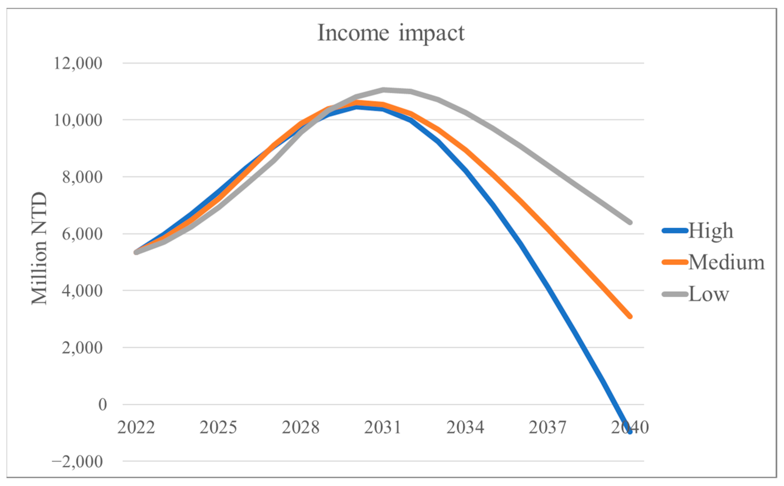
4.1. Economic Impacts

The output, income, and employment multipliers indicate the degree to which every NTD million that is invested affects the output, income, and employment, respectively. The results corresponding to each multiplier are illustrated below and summarized in

Table 6. Multiplier value and ranking of each industry.

Industry	Output	Rank	Income	Rank	Employment	Rank
Farming and Agri-food	1.86	10	0.35	7	0.84	2
Textile	1.95	6	0.37	5	0.61	3
Wood and Paper	1.81	13	0.33	11	0.53	6
Chemicals, Rubber, Plastic	1.90	8	0.22	15	0.28	18
Mineral Products	1.84	11	0.35	6	0.46	10
Metal and Metalworking	2.03	4	0.31	12	0.46	11
Electronic Components	1.50	14	0.18	19	0.26	19
Electronic Equipment	1.34	19	0.13	21	0.19	21
Machinery	1.87	9	0.33	10	0.49	8
Manufacture of ICEV	1.84	12	0.27	13	0.40	14
Manufacture of Other Transportation	2.01	5	0.34	8	0.46	12
Other Manufacturing	1.47	16	0.20	17	0.32	17
Electricity, Gas, Water	1.42	18	0.19	18	0.21	20
Construction	2.08	3	0.43	4	0.92	1
Wholesale and Retail	1.33	20	0.50	2	0.53	5
Transportation	1.49	15	0.34	9	0.52	7
Services	1.45	17	0.48	3	0.57	4
Administration	1.29	21	0.56	1	0.35	16
HEV	2.31	1	0.27	14	0.48	9
PHEV	2.12	2	0.22	16	0.43	13
BEV	1.94	7	0.18	20	0.37	15

.

The value of output multipliers varies according to the industry; however, they generally fall between 1.29 and 2.31. The output multiplier values for the top five industries were as follows: HEV (2.31), PHEV (2.12), construction (2.08), metal and metalworking (2.03), and the fabrication of other forms of transport (2.01). The output multiplier of BEVs was 1.94 (ranked 7th). These results indicate that the impact of EV-related industries in driving output value exceeds that of other industries. It is expected that by 2040, the EV industry will drive output of NTD 157~186.7 billion. The net output value will increase by NTD 77.9~97.5 billion, attributable to replacing ICEVs with a corresponding number of EVs.

Income multiplier values generally fall between 0.13 and 0.56. In the current study, the income multiplier values for the top five industries were as follows: administration (0.56), wholesale and retail (0.50), services (0.48), construction (0.43), and textile (0.37). These high values can be attributed to the high income coefficients in the above industries. Note, however, that the income multiplier values of the three EV industries were only 0.18~0.27 (ranked 14, 16, and 20, respectively). Thus, it is expected that by 2030, the EV industry will generate roughly NTD 10.5~10.8 billion in income; however, this will drop to NTD –0.9~6.4 billion by 2040. This can be attributed to the fact that HEVs have a higher income coefficient than ICEVs, which exceeds that of BEVs (i.e., HEVs > ICEVs > BEVs). Furthermore, the scenario setting results in an initial rapid increase in the number of HEVs, to be surpassed later by the number of BEVs. Thus, the income impact during the simulation period shows a trend from rise to decline.

Employment multiplier values generally fall between 0.19 and 0.92. In the current study, the employment multiplier values for the top five industries were as follows: construction (0.92), farming and agri-food (0.84), textiles (0.61), services (0.57), and wholesale and retail (0.53). These high values can be attributed to the fact that these sectors are labor-intensive. The three EV industries were ranked 9, 13, and 15, respectively. Compared with ICEVs, the difference in employment multiplier is not obvious. By 2040, the EV industry is expected to generate 19,700~26,700 job opportunities. Figure 1, Figure 2 and Figure 3 illustrate the impact on output, income, and employment under the three scenarios.

The impact of output, income, and employment on the various industries differed little among the scenarios. The industry that was most profoundly impacted was electronic equipment, followed by metal and metalworking, chemicals, rubber, plastic, and wholesale and retail.

It is expected that the introduction of EVs will reduce energy expenditures by NTD 53.8~60.5 billion by 2040, 34% of which (NTD 12.7~25.1 billion) can be attributed to HEVs, 5% of which (NTD 2.2~3.7 billion) can be attributed to PHEVs, and 61% of which (NTD 26.4~44.1 billion) can be attributed to BEVs. Figure 4 and Figure 5 present a comparison of the energy expenditures attributable to the various EVs under the three scenarios.

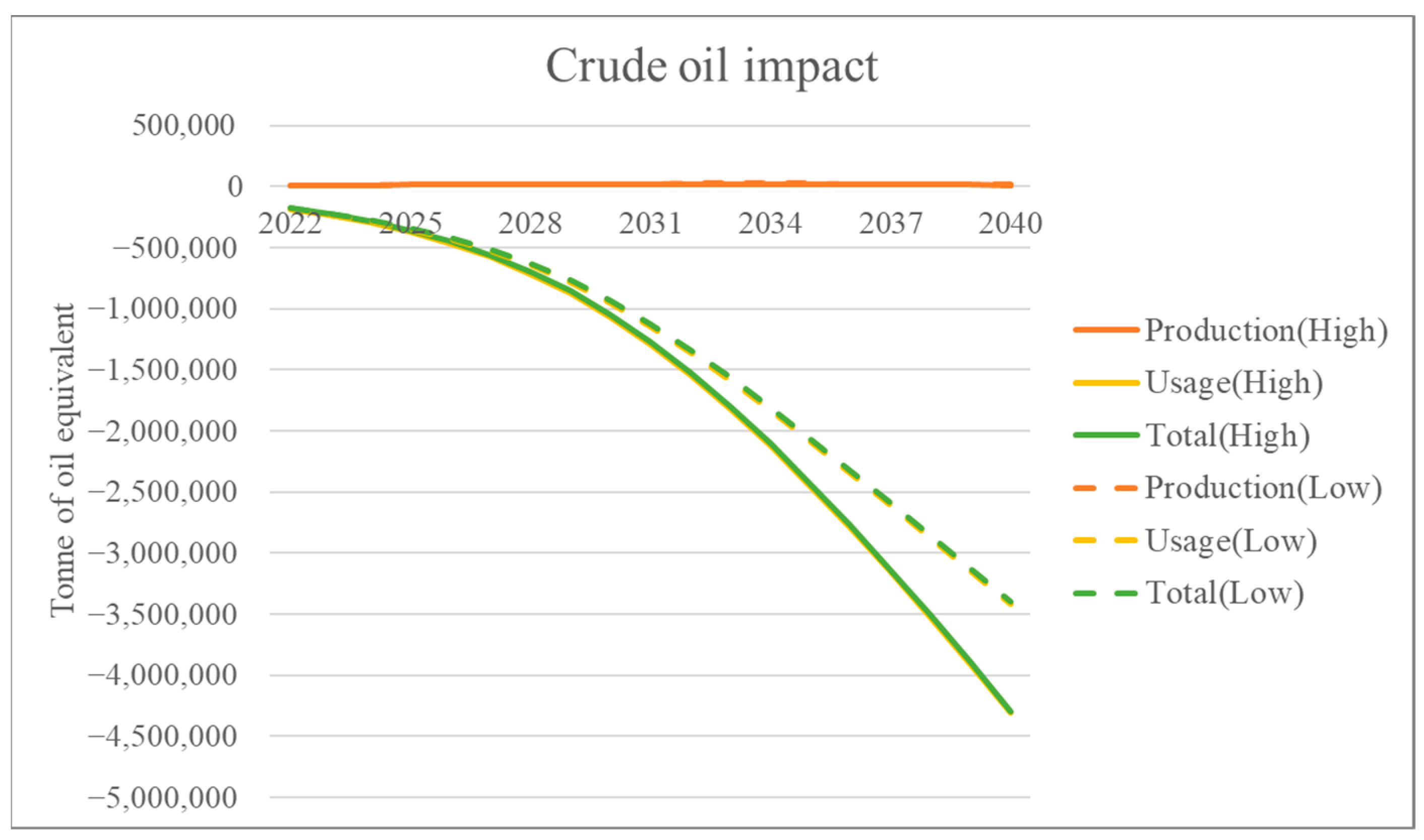
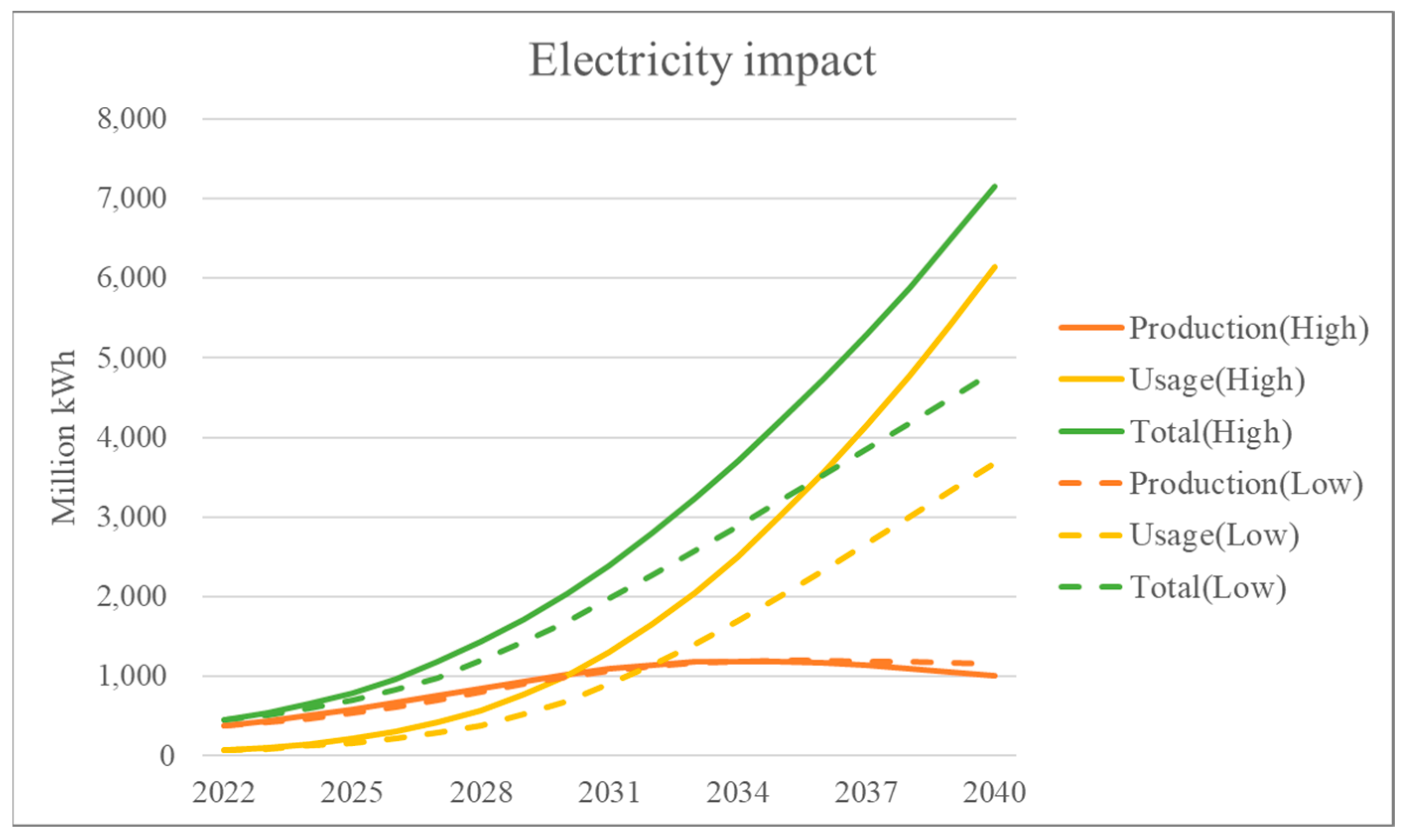
4.2. Impact of EVs on Energy Consumption

In this section, we examine the impact of EVs on energy consumption (crude oil and electricity) in terms of EV production and EV usage. The two values will then be combined to obtain the total impact of EVs on energy consumption (see Figure 6 and Figure 7).

The line indicating the impact on crude oil consumption of using EVs is close to that of the overall impact, due to the fact that the impacts of producing EVs are not significant. By 2040, the introduction of EVs is expected to reduce the consumption of crude oil by 3.42~4.31 million tons of oil equivalent (toe), which represents a 29~36% decrease in the consumption of crude oil in the transportation sector, while EV production will increase the consumption of crude oil by 10,100 to 18,900 toe. The combination of these two impacts is expected to achieve a 9~12% decrease in final consumption.

The effect on electricity consumption of manufacturing EVs will initially be more pronounced than the effect of using them; however, with the increase in the availability of EVs, the effects of EV usage are expected to exceed those of production by 2030 to 2032. By 2040, producing EVs will drive up electricity consumption by 1.0~1.2 billion kWh, while using EVs will drive up electricity consumption by 3.7~6.1 billion kWh; thus, total electricity consumption will increase by 4.8~7.1 billion kWh (2.08~3.08%).

If we normalize the consumption of crude oil and electricity by using the same unit, we find that the energy efficiencies of HEVs, PHEVs, and BEVs are, respectively, 1.62, 2.02, and 4.08 times higher than that of ICEVs. Overall, it appears that the introduction of EVs to Taiwan will reduce energy consumption in the transportation sector by 65~82% by 2040.

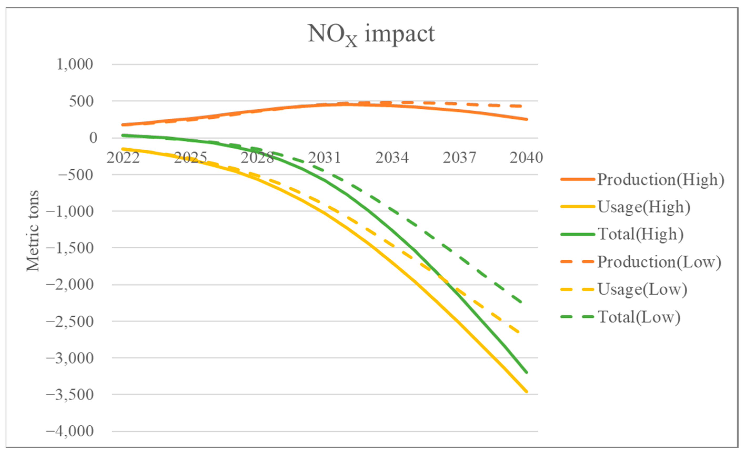
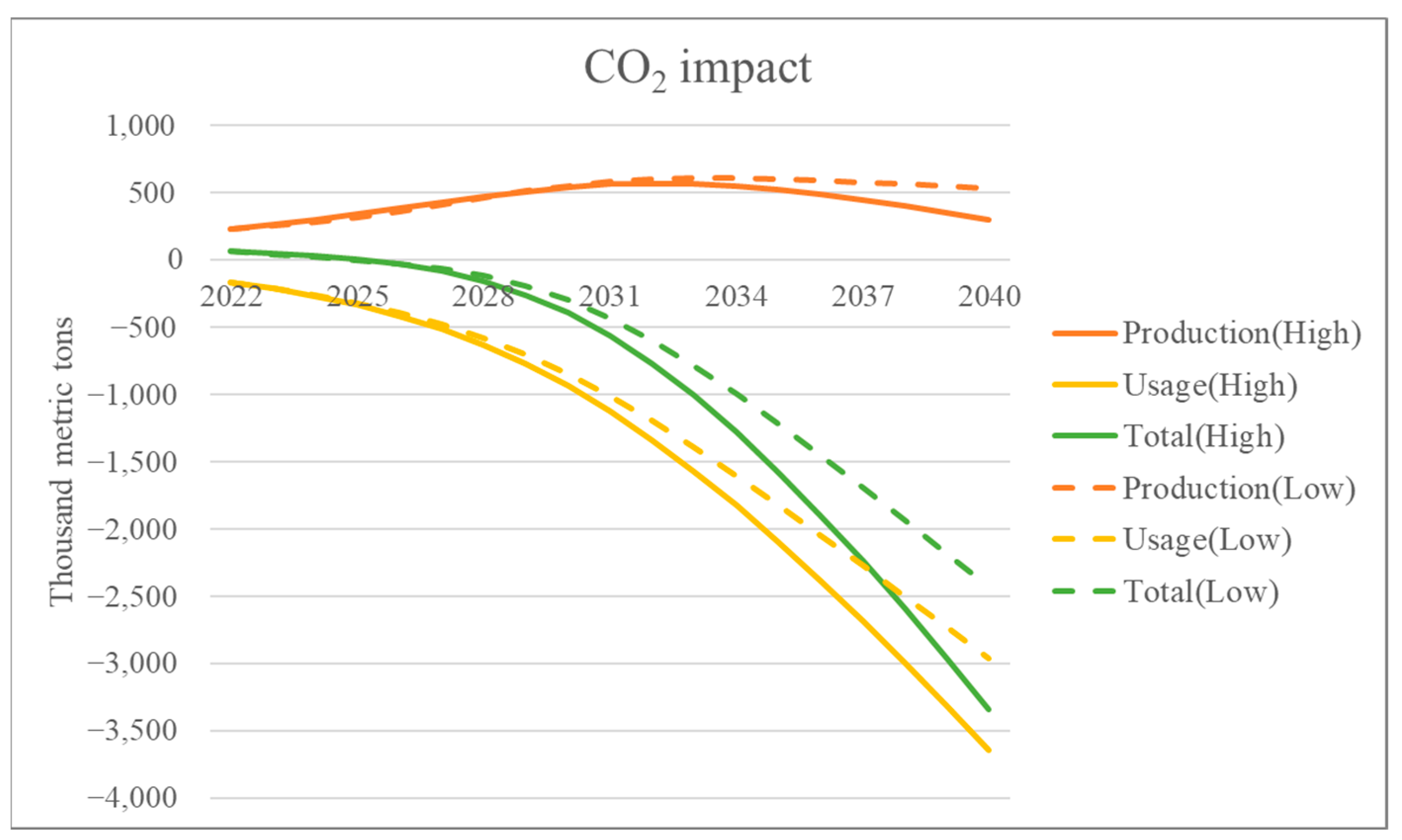
4.3. Environment Impacts

In this section, we examine the impact of EVs on the atmosphere, including CO₂, PM2.5, SO_X, and NO_X. As with the energy sector, we break down the impact of EVs into production and usage. The impact of manufacturing and using EVs on atmospheric pollutants is shown in Figure 8, Figure 9, Figure 10 and Figure 11.

Producing EVs will increase CO₂ emissions; however, using EVs will reduce CO₂ emissions. Note that the effect of producing EVs will be particularly evident in the sectors of electricity, gas, water, which should account for 66% of the effect. The effect of manufacturing EVs on CO₂ emissions will initially be more pronounced than the effect of using them; however, with the increase in the availability of EVs, the effects of EV usage are expected to exceed those of production by 2025 to 2026. By 2040, we will see a considerable decrease in CO₂ emissions (2432~3347 thousand metric tons, which is 6.86~9.44% of the CO₂ emissions in the transportation sector). Overall, it appears that the introduction of EVs to Taiwan (i.e., replacing an equivalent number of ICEVs) will reduce CO₂ emissions in the transportation sector by 12.79~17.61% by 2040.

The production of EVs is expected to increase atmospheric PM2.5 levels, while using EVs is expected to reduce these levels; however, the net result will be an increase in this pollutant. This can be attributed to the fact that PM2.5 emissions in manufacturing BEVs are 4.4 times higher than the PM2.5 emissions in manufacturing ICEVs, especially in battery manufacturing. In addition, the BEV industry is expected to grow enormously in the near future. Our results indicate that the emission of PM2.5 will increase by 63~96 metric tons by 2040, which represents a 5.76~8.78% increase attributable to replacing ICEVs with EVs.

The production of EVs is expected to increase atmospheric SO_X levels; however, the usage of EVs is expected to reduce SO_X levels, with overall SO_X emissions remaining at roughly the same level by 2040. In the production of EVs, most of the SO_X will be from the sectors of electricity, gas, water (30%) and metal and metalworking (30%). In using EVs, the initial decrease in SO_X emissions is expected to plateau at some point. This situation is similar to the impact of EVs on income, wherein the effect on reducing SO_X emissions will vary as follows: HEVs > ICEVs > BEVs. We are likely to see an initial rapid increase in the number of HEVs, to be surpassed later by the number of BEVs. Our results indicate that by 2040, SO_X emissions will decrease by 1~220 metric tons, which represents a decrease of 0.01~2.74% attributable to replacing ICEVs with a corresponding number of EVs.

Our results for NO_X are similar to of the result for CO₂, due to the fact that the emission coefficients of these pollutants are similar. In the production of EVs, most of the NO_X and CO₂ emissions will be from the sectors of electricity, gas, water (20%) and transportation (20%). Our results indicate that by 2040, NO_X emissions will decrease by 2298~3199 metric tons, which represents a decrease of 14.41~20.06% attributable to replacing ICEVs with a corresponding number of EVs.

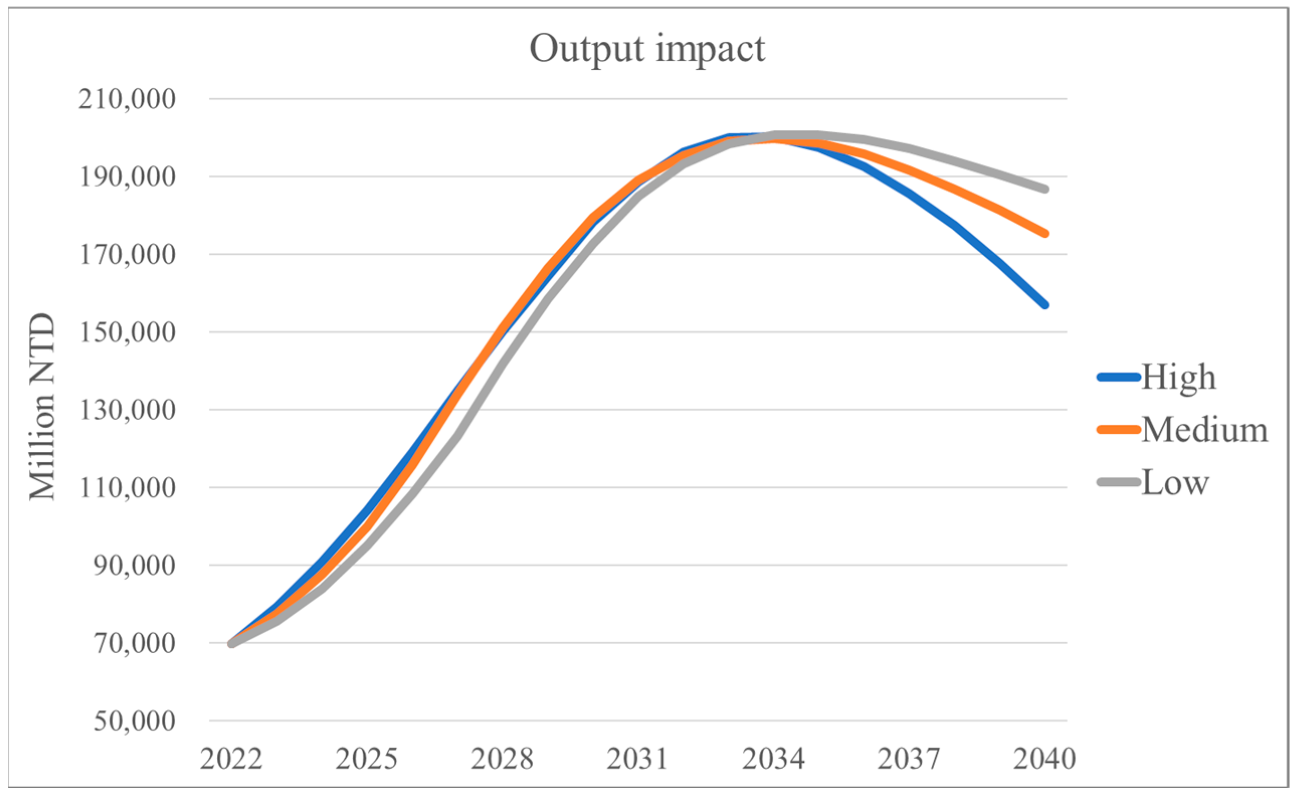
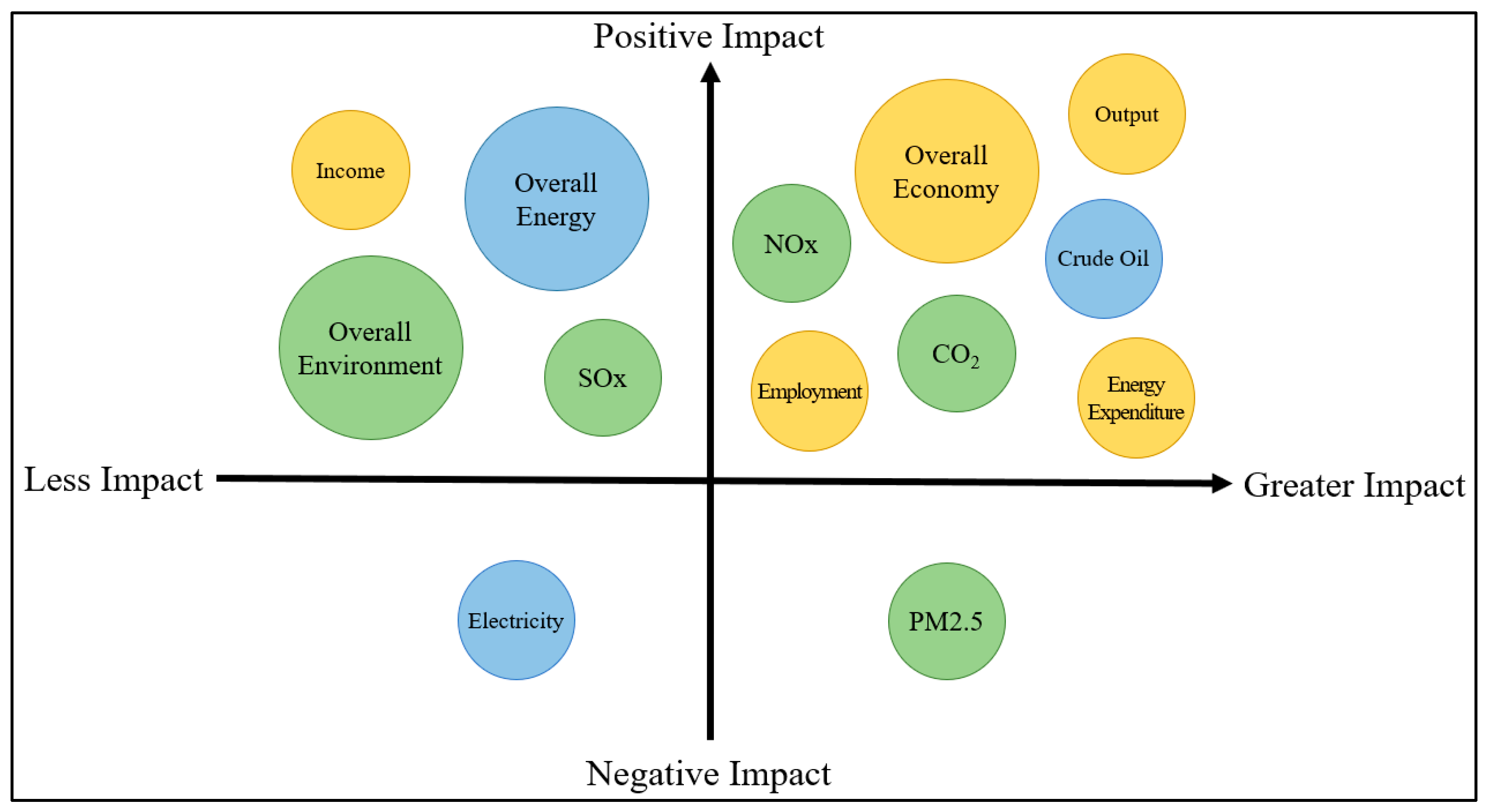
4.4. Economic–Energy–Environmental Impacts

The overall 3E effects of EVs are expected to be positive, with the most pronounced effects observed in economic indicators. Figure 12 presents a quadrant diagram illustrating the influential factors: Quadrant 1 (factors with a strongly positive impact), Quadrant 2 (factors with a weakly positive impact), Quadrant 3 (factors with a weakly negative impact), and Quadrant 4 (factors with a strongly negative impact). The yellow, blue, and green circles, respectively, indicate economic effects, energy-related effects, and environmental effects. All of the economic effects are expected to be positive; therefore, the overall economic impact is strongly positive (Quadrant 1). The energy efficiency of EVs is superior to that of ICEVs; however, there are still many electricity-related challenges that must be overcome (e.g., construction of charging facilities and enhancing the resilience of power plants and grids). Thus, the overall energy-related effect is weakly positive (Quadrant 2). According to the IQair World Air Quality Report 2022 [37], Taiwan ranked 76th in 2021 in terms of PM2.5 levels. The adoption of EVs is expected to have a profound impact on reducing environmental CO₂, NO_X, and SO_X; however, it is expected to increase PM2.5 levels. Taken together, the overall environmental impact of EV adoption is weakly positive (Quadrant 2).

Despite its valuable contributions, this paper is subject to several limitations and challenges.

• As an emerging industry, there is a lack of available data on the manufacture of EVs in Taiwan. Thus, in the current study, we were limited to the work of Suehiro and Purwanto [16] as data sources for the input structure. Until data pertaining to the domestic EV market become available, it will not be possible to derive specific input structures for Taiwan.
• The learning rates used in this study were derived from Weiss et al. [31,32]. In the future, it will be necessary to update the learning rate based on developments in the EV industry in Taiwan.
• An inherent limitation of the I–O method is its dependence on the selection of coefficients (e.g., the income coefficient). It is important to consider that these coefficients are static; i.e., they cannot account for import substitution, technological improvements, or relative changes in input prices over time. In the future, it should be possible to integrate the I–O model with an econometric model to reflect the dynamic nature of these effects.
• Capturing the distribution and flow of products among different industries in a given year through the construction of I–O tables takes a great deal of time. The latest I–O table (for 2016) was released in 2021. The inputs will need to be updated upon the release of the next I–O table.
• We were unable to obtain data pertaining to average vehicle performance in Taiwan; therefore, we adopted the most popular models as representative of overall vehicle performance. Note, also, that the technological improvements affecting energy efficiency were not considered in this study. These issues could be considered in future studies.

5. Conclusions and Policy Implications

In this study, we used I–O analysis to explore the cross-sectoral economic–energy–environmental impacts of EVs, using Taiwan as a case study. The EV industry possesses a high degree of backward linkages and a low degree of forward linkages, which means that it is largely unaffected by other industries and can easily drive development in other industries. In terms of economic impact, the output multiplier of the EV industry is relatively high. We estimate that by 2040, the output value of EVs will be NTD 157~186.7 billion, generating 19,700~26,700 job opportunities and reducing energy expenditure by NTD 53.8~60.5 billion. The development of the EV industry is not expected to have a profound effect on incomes; however, the overall economic impact should be positive.

By 2040, the development of the EV industry will reduce the final consumption of crude oil by 9~12% but increase the final consumption of electricity by 2.08~3.08%. Within the same period, the superior energy conversion efficiency of EVs (compared to ICEVs) is expected to reduce energy consumption in the transportation sector by 65~82%. The reduction in CO₂ and NO_X emissions through the ongoing usage of EVs should exceed the increase in CO₂ and NO_X emissions associated with the manufacture of these vehicles. Our results indicate that by 2040, the replacement of ICEVs with a corresponding number of EVs will reduce CO₂ emissions by 12.79~17.61% and NO_X emissions by 14.41~20.06%. The production of EVs is expected to increase atmospheric PM2.5 levels, while using EVs is expected to reduce these levels; the net result will be an increase in this pollutant. We expect that by 2040, replacing ICEVs with a corresponding number of EVs will increase the emission of PM2.5 by 63~96 metric tons (5.76~8.78%). Within the same time frame, we expect to see a 0.01~2.74% decrease in SO_X emissions attributable to EVs.

In accordance with our simulation results, we formulated three policy recommendations for reference in the context of efforts to promote the development and adoption of EVs.

• Strengthen the EV usage environment: Despite the seemingly inevitable widespread adoption of EVs, many consumers remain skeptical. Governments should proactively develop the infrastructure required for fast-charging systems in residences, companies, and public parking lots. Governments should also continue the provision of purchase subsidies to bolster the market shares of BEVs and PHEVs. For example, the Clean Vehicle Assistance Program (under Advanced Clean Cars II) in California provides low-income car buyers with down-payment subsidies of up to USD 5000 and favorable loan-interest rates. This program is backed by Governor Newsom’s USD $2.4 billion investment in vehicle incentives, the charging infrastructure, and public outreach programs.
• Promote the development and manufacture of EVs in Taiwan: The bourgeoning EV industry has enormous economic potential, particularly in terms of EV components, batteries, and the charging infrastructure. At present, Taiwan relies almost exclusively on imported EV batteries. Retaining the benefits of this transition will require Taiwan to develop domestic EV-battery technology. Therefore, we recommend that governments assist the domestic automobile industry in expanding production capacity. It is also expected that EV development will have a profound impact on the ICEV industry. Therefore, we recommend that governments enhance the resilience of domestic manufacturers by providing technical and financial support to promote the transformation of ICEVs. As an example, consider the subsidies for the EV industry in Austria. The Austrian Research Promotion Agency provides a 14% research tax credit to companies that are engaged in the technology development of EVs. The Austrian government has also established a “Climate and Energy Fund”, which provides financial support (grants of EUR 30,000 to EUR 750,000) to companies engaged in environmental and energy research.
• Strengthen the power supply and grid: A transition to EVs will inevitably increase demand for electricity and peak load levels, with a corresponding increase in pollution emissions. Governments should schedule the construction of new power-generation facilities and the decommissioning of outdated systems, as well as conduct rolling adjustments to compensate suppliers for changes in the demand for power. It is also important to continue the development of renewable energy to reduce emissions. One approach to overcoming the problem of peak load is to establish a payment mechanism aimed at spreading out the temporal distribution of EV-charging-station usage. Governments should also seek to strengthen energy-storage systems and vehicles-to-grid (V2G) technology to enhance the stability of the power grid.

References

1. REN21. Renewables 2023 Global Status Report. Available online: https://www.ren21.net/gsr-2023/ (accessed on 1 September 2023).
2. IEA. Global EV Outlook 2023. Available online: https://www.iea.org/reports/global-ev-outlook-2023 (accessed on 1 September 2023).
3. National Development Council. Taiwan’s Pathway to Net-Zero Emissions in 2050. Available online: https://www.ndc.gov.tw/en/Content_List.aspx?n=B154724D802DC488 (accessed on 31 December 2022).
4. Yang, L.; Yu, B.; Yang, B.; Chen, H.; Malima, G.; Wei, Y.M. Life cycle environmental assessment of electric and internal combustion engine vehicles in China. J. Clean. Prod. 2021, 285, 124899. [Google Scholar] [CrossRef]
5. Hussain, A.; Ullah, K.; Senapati, T.; Moslem, S. Complex spherical fuzzy Aczel Alsina aggregation operators and their application in assessment of electric cars. Heliyon 2023, 9, e18100. [Google Scholar] [CrossRef]
6. Mauler, L.; Duffner, F.; Zeier, W.G.; Lekerad, J. Battery cost forecasting: A review of methods and results with an outlook to 2050. Energy Environ. Sci. 2021, 14, 4712–4739. [Google Scholar] [CrossRef]
7. Leontief, W.W. Quantitative input and output relations in the economic systems of the United States. Rev. Econ. Stat. 1936, 18, 105–125. [Google Scholar] [CrossRef]
8. Lian, Y.W. Research on input-output analysis of transportation industry in Taiwan. Bank Taiwan Q. 1986, 37, 144–185. [Google Scholar]
9. Wang, T.F. Economic effect analysis of Taiwan’s transportation and communication construction. Taipei Econ. Inq. 1990, 30, 79–125. [Google Scholar]
10. Nir, A.S.; Liang, G.S. Transport sector construction inter-industry effects positive study in Taiwan area. Marit. Res. J. 2003, 14, 1–28. [Google Scholar]
11. Chen, H.C. Analysis of the Influence on Economy of Kaohsiung Metropolis Caused by the Constructure of Mass Rapid Transmit. Master’s Thesis, Institute of Economics, National Sun Yat-sen University, Kaohsiung City, Taiwan, 2004. [Google Scholar]
12. Lin, G.Y. The Initially Researches to Economic Activity and the Mobility Behavior of Passengers in Taiwan during High Speed Rail (HSR) Construction and Transport. Master’s Thesis, Institute of Public Affairs Management, National Sun Yat-sen University, Kaohsiung City, Taiwan, 2011. [Google Scholar]
13. Mead, D. The impact of the electric car on the U.S. economy: 1998–2005. Econ. Syst. Res. 1995, 7, 413–438. [Google Scholar] [CrossRef]
14. Leurent, F.; Windisch, E. Benefits and costs of electric vehicles for the public finances: An integrated valuation model based on input-output analysis, with application to France. Res. Transp. Econ. 2015, 50, 51–62. [Google Scholar] [CrossRef]
15. Ulrich, P.; Lehr, U. Economic effects of an e-mobility scenario—input structure and energy consumption. Econ. Syst. Res. 2020, 32, 84–97. [Google Scholar] [CrossRef]
16. Suehiro, S.; Purwanto, A.J. The Influence on Energy and the Economy of Electrified Vehicles Penetration in ASEAN; ERIA Research Project Report 2020, No. 14; ERIA: Jakarta, Indonesia, 2020. [Google Scholar]
17. Nagashimaa, S.; Uchiyamaa, Y.; Okajima, K. Environment, energy and economic analysis of wind power generation system installation with input-output table. Energy Procedia 2015, 75, 683–690. [Google Scholar] [CrossRef]
18. Hienuki, S.; Kudoh, Y.; Hondo, H. Life cycle employment effect of geothermal power generation using an extended input-output model: The case of Japan. J. Clean. Prod. 2015, 93, 203–212. [Google Scholar] [CrossRef]
19. Varela-Vazquez, P.; Sanchez-Carreira, M.C. Estimation of the potential effects of offshore wind on the Spanish economy. Renew. Energy 2017, 111, 815–824. [Google Scholar] [CrossRef]
20. Nakanoa, S.; Araib, S.; Washizuc, A. Development and application of an inter-regional input-output table for analysis of a next generation energy system. Renew. Sustain. Energy Rev. 2018, 82, 2834–2842. [Google Scholar] [CrossRef]
21. Bekel, K.; Pauliuk, S. Prospective cost and environmental impact assessment of battery and fuel cell electric vehicles in Germany. Int. J. Life Cycle Assess. 2019, 24, 2220–2237. [Google Scholar] [CrossRef]
22. Lombardi, L.; Tribioli, L.; Cozzolino, R.; Bella, G. Comparative environmental assessment of conventional, electric, hybrid, and fuel cell powertrains based on LCA. Int. J. Life Cycle Assess. 2017, 22, 1989–2006. [Google Scholar] [CrossRef]
23. Yan, X.; Sun, S. Impact of electric vehicle development on China’s energy consumption and greenhouse gas emissions. Clean Technol. Environ. Policy 2021, 23, 2909–2925. [Google Scholar] [CrossRef]
24. Das, J. Comparative life cycle GHG emission analysis of conventional and electric vehicles in India. Environ. Dev. Sustain. 2022, 24, 13294–13333. [Google Scholar] [CrossRef]
25. Hofmann, J.; Guan, D.; Chalvatzis, K.; Huo, H. Assessment of electrical vehicles as a successful driver for reducing CO2 emissions in China. Appl. Energy 2016, 184, 995–1003. [Google Scholar] [CrossRef]
26. Liu, D.; Xu, L.; Sadia, U.H.; Wang, H. Evaluating the CO2 emission reduction effect of China’s battery electric vehicle promotion efforts. Atmos. Pollut. Res. 2021, 12, 101115. [Google Scholar] [CrossRef]
27. Winyuchakrit, P.; Sukamongkol, Y.; Limmeechokchai, B. Do electric vehicles really reduce GHG emissions in Thailand? Energy Procedia 2017, 138, 348–353. [Google Scholar] [CrossRef]
28. Directorate General of Budget, Accounting and Statistics, Executive Yuan. The Report on 2016 Input-Output Statistics; Executive Yuan: Taipei, Taiwan, 2020. [Google Scholar]
29. IEA. Global EV Outlook 2022. Available online: https://www.iea.org/reports/global-ev-outlook-2022 (accessed on 31 January 2023).
30. Wright, T.P. Factors affecting the cost of airplanes. J. Aeronaut. Sci. 1936, 3, 122–128. [Google Scholar] [CrossRef]
31. Weiss, M.; Patel, M.K.; Junginger, M.; Perujo, A.; Bonnel, P.; Grootveld, G. On the electrification of road transport-Learning rates and price forecasts for hybrid-electric and battery-electric vehicles. Energy Policy 2012, 48, 374–393. [Google Scholar] [CrossRef]
32. Weiss, M.; Zerfass, A.; Helmers, E. Fully electric and plug-in hybrid cars—An analysis of learning rates, user costs, and costs for mitigating CO2 and air pollutant emissions. J. Clean. Prod. 2019, 212, 1478–1489. [Google Scholar] [CrossRef]
33. Bureau of Energy BOE. Energy Statistics Handbook 2019; Bureau of Energy, Ministry of Economic Affairs: Taipei, Taiwan, 2019. [Google Scholar]
34. Kim, H.C.; Wallington, T.J.; Mueller, S.A.; Bras, B.; Guldberg, T.; Tejada, F. Life cycle water use of ford focus gasoline and ford focus electric vehicles. J. Ind. Ecol. 2015, 20, 1122–1133. [Google Scholar] [CrossRef]
35. Bureau of Energy BOE. 2020 Vehicle Fuel Economy Guide; Bureau of Energy, Ministry of Economic Affairs: Taipei, Taiwan, 2021. [Google Scholar]
36. Environmental Protection Agency. Taiwan Emission Data System; Environmental Protection Agency: Taipei, Taiwan, 2021. [Google Scholar]
37. IQAir. 2022 World Air Quality Report. 2022. Available online: https://www.iqair.com/us/world-air-quality-report#msdynttrid=BScYH7jfCKlFL5Cb54-VR2LvdUe3v8vK_IbtpA5mzLY (accessed on 1 September 2023).
Figure 1. Impact of EV adoption on output under each scenario.
Sustainability 15 14135 g001
Figure 2. Impact of EV adoption on income under each scenario.
Sustainability 15 14135 g002
Figure 3. Impact of EV adoption on employment under each scenario.
Sustainability 15 14135 g003
Figure 4. Comparison of energy expenditures of electric vehicle type under each scenario.
Sustainability 15 14135 g004
Figure 5. Comparison of total energy expenditures under each scenario.
Sustainability 15 14135 g005
Figure 6. Impact of EV adoption on crude oil under each scenario.
Sustainability 15 14135 g006
Figure 7. Impact of EV adoption on electricity under each scenario.
Sustainability 15 14135 g007
Figure 8. Impact of EV adoption on CO2 under each scenario.
Sustainability 15 14135 g008
Figure 9. Impact of EV adoption on PM2.5 under each scenario.
Sustainability 15 14135 g009
Figure 10. Impact of EV adoption on SOX under each scenario.
Sustainability 15 14135 g010
Figure 11. Impact of EV adoption on NOX under each scenario.
Sustainability 15 14135 g011
Figure 12. Quadrant diagram characterizing the influence of the various factors on the 3Es.
Sustainability 15 14135 g012