
Optimization of the Uniformity Index Performance in the Selective Catalytic Reduction System Using a Metamodel

Abstract
:1. Introduction
2. Methodology
2.1. SCR System and Numerical Analysis
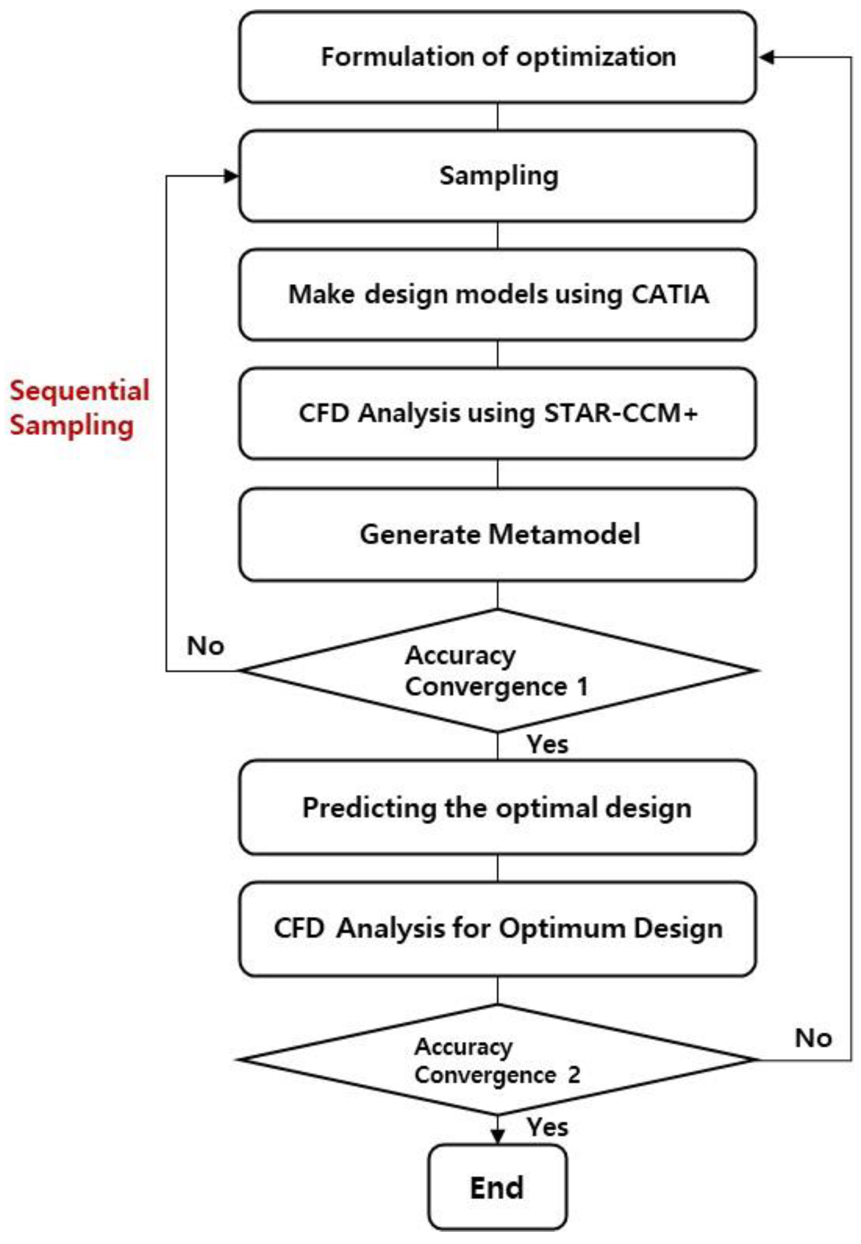
2.2. Formulation of Optimization
3. Results of Optimization
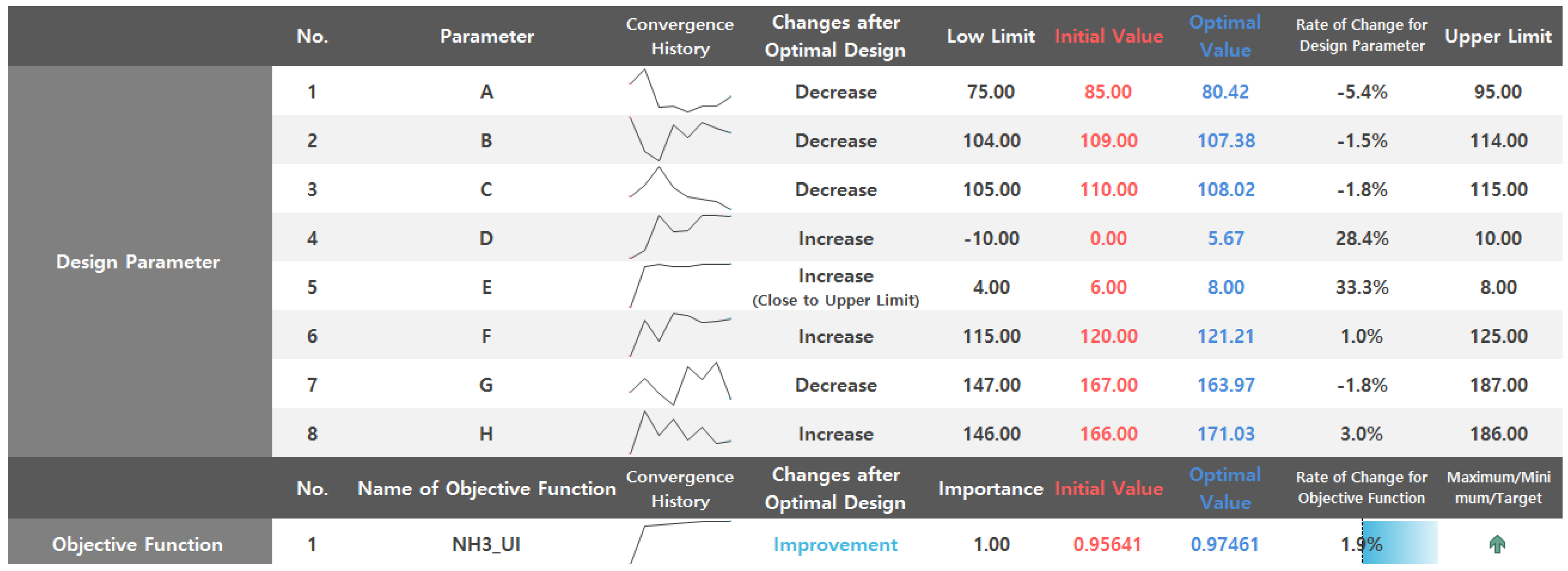
3.1. Optimization with the Metamodel
3.2. Comparison of Results
4. Conclusions
Author Contributions
Funding
Institutional Review Board Statement
Informed Consent Statement
Data Availability Statement
Acknowledgments
Conflicts of Interest
Abbreviations
| SCR | Selective Catalytic Reduction |
| UI | Uniformity Index |
| EDT | Ensemble Decision Tree |
| RBFi | Radial Basis Function Interpolation |
| RBFr | Radial Basis Function Regression |
| RMSE | Root Mean Square Error |
| Norm. RMSE | Normalized Root Mean Square Error |
| Max. Abs. Error | Maximum Absolute Error |
| DOE | Design of Experiments |
| MLO | Multi-start Local Optimization |
| QBC | Query-by-Commitment |
| MMDS | Multiple Maximum Distance Sampling |
| CFD | Computational Fluid Dynamics |
| MLE | Maximum Likelihood Estimation |
Appendix A

| No. | A | B | C | D | E | F | G | H | NH3 UI |
|---|---|---|---|---|---|---|---|---|---|
| Case 1 | 95 | 114 | 115 | 10 | 8 | 125 | 187 | 186 | 0.964 |
| Case 2 | 95 | 114 | 115 | −10 | 4 | 115 | 187 | 146 | 0.833 |
| Case 3 | 95 | 109 | 110 | 10 | 8 | 125 | 167 | 166 | 0.966 |
| Case 4 | 95 | 109 | 110 | 0 | 6 | 120 | 167 | 146 | 0.943 |
| Case 5 | 95 | 109 | 110 | −10 | 4 | 115 | 167 | 186 | 0.867 |
| Case 6 | 95 | 104 | 105 | 0 | 6 | 120 | 147 | 186 | 0.962 |
| Case 7 | 85 | 109 | 105 | 0 | 4 | 125 | 187 | 166 | 0.851 |
| Case 8 | 85 | 109 | 105 | −10 | 8 | 120 | 187 | 146 | 0.963 |
| Case 9 | 85 | 104 | 115 | 10 | 6 | 115 | 167 | 166 | 0.955 |
| Case 10 | 85 | 104 | 115 | 0 | 4 | 125 | 167 | 146 | 0.853 |
| Case 11 | 85 | 104 | 115 | −10 | 8 | 120 | 167 | 186 | 0.970 |
| Case 12 | 85 | 114 | 110 | 10 | 6 | 115 | 147 | 146 | 0.951 |
| Case 13 | 85 | 114 | 110 | −10 | 8 | 120 | 147 | 166 | 0.964 |
| Case 14 | 75 | 104 | 110 | 10 | 4 | 120 | 187 | 186 | 0.874 |
| Case 15 | 75 | 104 | 110 | 0 | 8 | 115 | 187 | 166 | 0.973 |
| Case 16 | 75 | 104 | 110 | −10 | 6 | 125 | 187 | 146 | 0.943 |
| Case 17 | 75 | 114 | 105 | 0 | 8 | 115 | 167 | 146 | 0.966 |
| Case 18 | 75 | 114 | 105 | −10 | 6 | 125 | 167 | 186 | 0.956 |
| Case 19 | 75 | 109 | 115 | 0 | 8 | 115 | 147 | 186 | 0.968 |
| No. | A | B | C | D | E | F | G | H | NH3 UI |
|---|---|---|---|---|---|---|---|---|---|
| Case 20 | 95 | 104 | 115 | 10 | 4 | 125 | 187 | 146 | 0.894 |
| Case 21 | 79.11 | 112.13 | 106.63 | 3.87 | 7 | 122.24 | 152.07 | 158.89 | 0.966 |
| Case 22 | 92.33 | 108.93 | 113.6 | −9.33 | 7 | 122.25 | 170.47 | 158 | 0.967 |
| Case 23 | 78.35 | 108.47 | 108.4 | −8.54 | 6 | 116.98 | 170.45 | 166.11 | 0.965 |
| Case 24 | 77.93 | 105.93 | 106.05 | 4 | 6 | 122.13 | 148.65 | 172.39 | 0.964 |
| Case 25 | 89.92 | 110.41 | 112.17 | 9.15 | 6 | 115.27 | 153.42 | 165.26 | 0.963 |
| Case 26 | 75 | 114 | 105 | 10 | 4 | 125 | 187 | 146 | 0.906 |
| Case 27 | 90.6 | 104.4 | 107.58 | 0.83 | 5 | 118.87 | 173.93 | 177.7 | 0.957 |
| Case 28 | 80.37 | 109.27 | 107.07 | −7.37 | 4 | 120.66 | 185.4 | 179.87 | 0.916 |
| Case 29 | 94.05 | 113.49 | 105.67 | −0.92 | 6 | 124.04 | 183.44 | 182.53 | 0.916 |
| Case 30 | 81.93 | 113.53 | 107.74 | −6.93 | 4 | 118.73 | 148.4 | 149.64 | 0.931 |
| Case 31 | 89.8 | 110.6 | 113.63 | 2.72 | 5 | 124.67 | 162.73 | 178.54 | 0.951 |
| Case 32 | 76.18 | 112.24 | 106.76 | −0.59 | 5 | 120.29 | 163.23 | 171.88 | 0.954 |
| Case 33 | 77.35 | 108.12 | 112.65 | 6.49 | 6 | 117.35 | 184.65 | 181.29 | 0.962 |
| Case 34 | 82.05 | 109.3 | 111.47 | 9.99 | 5 | 123.23 | 182.28 | 157.76 | 0.944 |
| Case 35 | 82.06 | 109.29 | 109.12 | −8.82 | 6 | 115 | 170.53 | 155.41 | 0.961 |
| Case 36 | 84.41 | 106.35 | 113.24 | 6.47 | 7 | 119.89 | 156.41 | 183.65 | 0.969 |
| Case 37 | 85.59 | 110.47 | 114.41 | 5.29 | 4 | 118.53 | 160.13 | 150.71 | 0.918 |
| Case 38 | 90.29 | 111.06 | 110.29 | 8.82 | 5 | 116.77 | 172.88 | 178.03 | 0.952 |
| Case 39 | 92.65 | 104.01 | 106.76 | −6.47 | 7 | 118.49 | 147.01 | 167.16 | 0.968 |
| No. | A | B | C | D | E | F | G | H | NH3 UI |
|---|---|---|---|---|---|---|---|---|---|
| Case 40 | 75.00 | 107.13 | 109.38 | 6.25 | 8 | 121.31 | 174.50 | 171.00 | 0.975 |
| Case 41 | 84.33 | 104.33 | 111.84 | 7.47 | 7 | 121.10 | 170.19 | 180.83 | 0.970 |
| Case 42 | 94.00 | 111.83 | 110.93 | −7.88 | 8 | 118.33 | 160.34 | 183.84 | 0.973 |
| Case 43 | 87.66 | 109.34 | 112.34 | −1.44 | 6 | 116.43 | 184.86 | 172.18 | 0.961 |
| Case 44 | 93.54 | 112.13 | 114.74 | 5.95 | 5 | 124.45 | 165.67 | 160.41 | 0.947 |
| Case 45 | 87.32 | 110.40 | 106.93 | −4.01 | 7 | 121.29 | 174.20 | 185.27 | 0.971 |
| Case 46 | 78.24 | 105.72 | 111.10 | 6.62 | 7 | 120.40 | 164.60 | 153.32 | 0.966 |
| Case 47 | 81.87 | 105.79 | 106.20 | 2.93 | 7 | 117.65 | 185.81 | 171.87 | 0.970 |
| Case 48 | 93.98 | 110.13 | 112.46 | −2.90 | 8 | 119.14 | 181.93 | 152.67 | 0.968 |
| Case 49 | 76.49 | 107.40 | 107.80 | 4.20 | 7 | 118.87 | 155.80 | 181.46 | 0.973 |
| Case 50 | 92.45 | 110.15 | 105.30 | −8.39 | 5 | 124.13 | 149.92 | 176.13 | 0.959 |
| Case 51 | 79.66 | 104.73 | 112.55 | 10.00 | 4 | 124.67 | 155.59 | 174.99 | 0.939 |
| Case 52 | 85.92 | 109.93 | 110.61 | −0.67 | 5 | 115.93 | 149.56 | 172.15 | 0.958 |
| Case 53 | 94.73 | 107.80 | 106.27 | 1.41 | 4 | 121.33 | 147.74 | 150.81 | 0.930 |
| Case 54 | 94.73 | 107.33 | 105.50 | 2.02 | 6 | 116.87 | 159.27 | 154.05 | 0.960 |
| Case 55 | 86.73 | 106.41 | 108.80 | −8.81 | 5 | 120.13 | 161.13 | 185.17 | 0.955 |
| Case 56 | 90.78 | 112.20 | 110.46 | 9.60 | 5 | 116.82 | 173.40 | 160.13 | 0.949 |
| Case 57 | 82.90 | 112.70 | 108.34 | 3.33 | 4 | 123.89 | 149.87 | 170.53 | 0.933 |
| Case 58 | 79.40 | 106.99 | 105.41 | 9.60 | 5 | 119.00 | 176.06 | 183.88 | 0.954 |
| Case 59 | 87.27 | 106.32 | 107.20 | 9.06 | 8 | 119.01 | 154.99 | 150.81 | 0.968 |
| No. | A | B | C | D | E | F | G | H | NH3 UI |
|---|---|---|---|---|---|---|---|---|---|
| Case 60 | 95.00 | 104.15 | 115.00 | −9.59 | 4 | 115.00 | 185.37 | 186.00 | 0.907 |
| Case 61 | 80.30 | 109.09 | 110.93 | 1.54 | 6 | 118.65 | 168.55 | 167.33 | 0.963 |
| Case 62 | 79.77 | 108.36 | 112.59 | −8.52 | 7 | 125.00 | 151.87 | 164.69 | 0.965 |
| Case 63 | 92.74 | 107.05 | 105.00 | −4.13 | 6 | 119.74 | 180.55 | 149.48 | 0.955 |
| Case 64 | 91.91 | 106.28 | 109.43 | −1.43 | 6 | 125.00 | 163.50 | 158.92 | 0.958 |
| Case 65 | 81.89 | 109.38 | 105.55 | 2.72 | 4 | 119.40 | 181.67 | 157.55 | 0.912 |
| Case 66 | 78.50 | 107.82 | 110.45 | −8.00 | 5 | 122.52 | 171.27 | 185.73 | 0.956 |
| Case 67 | 75.21 | 107.54 | 111.39 | 10.00 | 8 | 123.73 | 187.00 | 150.13 | 0.970 |
| Case 68 | 92.47 | 114.00 | 109.20 | 1.30 | 7 | 116.23 | 187.00 | 163.95 | 0.967 |
| Case 69 | 75.12 | 107.91 | 105.98 | 4.40 | 6 | 116.00 | 181.99 | 186.00 | 0.967 |
| Case 70 | 80.99 | 104.00 | 109.27 | 9.23 | 4 | 115.00 | 182.54 | 164.13 | 0.919 |
| Case 71 | 82.85 | 110.64 | 114.97 | 1.46 | 8 | 115.44 | 147.00 | 146.00 | 0.962 |
| Case 72 | 75.25 | 106.40 | 115.00 | −10.00 | 6 | 123.69 | 168.34 | 164.43 | 0.960 |
| Case 73 | 89.27 | 109.79 | 113.13 | −4.23 | 5 | 117.72 | 166.33 | 176.41 | 0.953 |
| Case 74 | 75.00 | 109.68 | 113.21 | 2.79 | 6 | 120.27 | 183.22 | 171.52 | 0.961 |
| Case 75 | 95.00 | 112.46 | 112.34 | 9.54 | 5 | 125.00 | 183.33 | 172.67 | 0.944 |
| Case 76 | 89.98 | 112.41 | 107.63 | −3.03 | 6 | 121.32 | 170.63 | 164.14 | 0.962 |
| Case 77 | 85.41 | 114.00 | 111.84 | 6.03 | 7 | 123.98 | 161.83 | 161.77 | 0.964 |
| Case 78 | 95.00 | 106.40 | 108.55 | −1.02 | 8 | 120.07 | 167.55 | 175.93 | 0.972 |
| Case 79 | 81.39 | 111.45 | 109.64 | −2.66 | 5 | 120.34 | 147.00 | 156.92 | 0.954 |
| No. | A | B | C | D | E | F | G | H | NH3 UI |
|---|---|---|---|---|---|---|---|---|---|
| Case 1 | 95 | 114 | 115 | 0 | 6 | 120 | 187 | 166 | 0.941 |
| Case 2 | 95 | 104 | 105 | 10 | 8 | 125 | 147 | 146 | 0.960 |
| Case 3 | 95 | 104 | 105 | −10 | 4 | 115 | 147 | 166 | 0.880 |
| Case 4 | 85 | 109 | 105 | 10 | 6 | 115 | 187 | 186 | 0.950 |
| Case 5 | 85 | 114 | 110 | 0 | 4 | 125 | 147 | 186 | 0.880 |
| Case 6 | 75 | 114 | 105 | 10 | 4 | 120 | 167 | 166 | 0.874 |
| Case 7 | 75 | 109 | 115 | 10 | 4 | 120 | 147 | 146 | 0.875 |
| Case 8 | 75 | 109 | 115 | −10 | 6 | 125 | 147 | 166 | 0.956 |
| a. SCR System | |||
| No. | Classification | Unit | Value |
| 1 | Shell Material | SUS | 436 L |
| 2 | Mass Flow of Exhaust Gas | kg/h | 316 |
| 3 | Exhaust Gas Temp. | Max, °C | 411 |
| 4 | Turbo Charger | Max, RPM | 203,000 |
| 5 | Engine RPM | RPM | 3000 |
| 6 | AdBlue | mg/s | 105 |
| 7 | Urea Injection | mg/Injection | 30.6 |
| 8 | Injection Duration | msec | 81.6 |
| 9 | Pressure of Exhaust Gas | kPa | 9.8 |
| b. Urea injector nozzle holes | |||
| No. | Classification | Unit | Value |
| 1 | Number | No. | 3 |
| 2 | Hole Diameter | 120 | |
| 3 | Diameter at Hole Center Positions | mm | 1.9 |
| 4 | Circumferential Distribution | deg. | 120 |
| 5 | Static Mass Flow | kg/h | 3.2 |
| c. Injection initialization | |||
| No. | Classification | Unit | Value |
| 1 | Equivalent Spray Type | Type | 3-Hole Full Cone Spray |
| 2 | Cone Angle | deg. | 7 |
| 3 | Spray Angle | deg. | 7 |
| 4 | Estimated Initial Droplet Velocity | m/s | 24 |
| 5 | Droplet Diameter, SMD | μm | 100 |
| d. Information of Mesh modeling | |||
| No. | Classification | Value | No. |
| 1 | Analysis Tool | Star-CCM + V12.04 | 1 |
| 2 | Mesh Type | Polyhedral | 2 |
| 3 | Total Mesh Quantity | 1,041,308 | 3 |
| 4 | Base Mesh Size | 4 mm | 4 |
| 5 | Surface Mesh Size | 50~100% (Compared Base Mesh Size) | 5 |
| 6 | Number of Prism Layers | 3 | 6 |
| 7 | Prism Layer Thickness | 0.25 (Compared Base Thickness) | 7 |
| 8 | Fine Mesh | Surface: 25%, Prism: 12.5% | 8 |
References
- Zhang, Z.; Dong, R.; Tan, D.; Duan, L.; Jiang, F.; Yao, X.; Yang, D.; Hu, J.; Zhang, J.; Zhong, W.; et al. Effect of structural parameters on diesel particulate filter trapping performance of heavy-duty diesel engines based on grey correlation analysis. Energy 2023, 271, 127025. [Google Scholar] [CrossRef]
- Zhang, Z.; Dong, R.; Lan, G.; Yuan, T.; Tan, D. Diesel particulate filter regeneration mechanism of modern automobile engines and methods of reducing PM emissions: A review. Environ. Sci. Pollut. Res. 2023, 30, 39338–39376. [Google Scholar] [CrossRef] [PubMed]
- Kim, H.-S.; Kasipandi, S.; Kim, J.; Kang, S.-H.; Kim, J.-H.; Ryu, J.-H.; Bae, J.-W. Current Catalyst Technology of Selective Catalytic Reduction (SCR) for NOx Removal in South Korea. Catalysts 2021, 10, 52. [Google Scholar] [CrossRef]
- Kaźmierski, B.; Kapusta, J. The importance of individual spray properties in performance improvement of a urea-SCR system employing flash-boiling injection. Appl. Energy 2023, 329, 120217. [Google Scholar] [CrossRef]
- Wardana, M.; Oh, K.; Lim, O. Investigation of Urea Uniformity with Different Types of Urea Injectors in an SCR System. Catalysts 2020, 10, 1269. [Google Scholar] [CrossRef]
- Mehdi, G.; Zhou, S.; Zhu, Y.; Shah, A.H.; Chand, K. Numerical Investigation of SCR Mixer Design Optimization for Improved Performance. Processes 2019, 7, 168. [Google Scholar] [CrossRef]
- Jiao, Y.; Zheng, Q. Urea Injection and Uniformity of Ammonia Distribution in SCR System of Diesel Engine. Appl. Math. Nonlinear Sci. 2020, 5, 129–142. [Google Scholar] [CrossRef]
- Jeong, S.; Kim, H.; Kim, H.; Kwon, O.; Park, E.; Kang, J. Optimization of the Urea Injection Angle and Direction: Maximizing the Uniformity Index of a Selective Catalytic Reduction System. Energies 2020, 14, 157. [Google Scholar] [CrossRef]
- Park, K.; Hong, C.H.; Oh, S.; Moon, S. Numerical Prediction on the Influence of Mixer on the Performance of Urea-SCR System. World Acad. Sci. Eng. Technol. Int. J. Mech. Aerosp. Ind. Mechatron. Eng. 2014, 8, 972–978. [Google Scholar] [CrossRef]
- Ye, J.; Lv, J.; Tan, D.; Ai, Z.; Feng, Z. Numerical analysis on enhancing spray performance of SCR mixer device and heat transfer performance based on field synergy principle. Processes 2021, 9, 786. [Google Scholar] [CrossRef]
- Antony, J. Design of Experiments for Engineers and Scientists; Elsevier: Amsterdam, The Netherlands, 2014. [Google Scholar] [CrossRef]
- Hoang, P.H.; Phan, H.N.; Nguyen, D.T.; Paolacci, F. Kriging Metamodel-Based Seismic Fragility Analysis of Single-Bent Reinforced Concrete Highway Bridges. Buildings 2021, 11, 238. [Google Scholar] [CrossRef]
- Kim, S.E.; Yoo, Y.M. Optimization of a Permanent Magnet Synchronous Motor for e-Mobility Using Metamodels. Appl. Sci. 2022, 12, 1625. [Google Scholar] [CrossRef]
- You, Y.-M. Optimal Design of PMSM Based on Automated Finite Element Analysis and Metamodeling. Energies 2019, 12, 4673. [Google Scholar] [CrossRef]
- Chung, I.B.; Lee, Y.B.; Choi, D.H. Global metamodeling using sequential and adaptive sampling with two criteria for global exploration and local exploitation. Korean Soc. Mech. Eng. 2020, 170–175. [Google Scholar]
- Shin, Y.S.; Lee, Y.B.; Ryu, J.S.; Choi, D.H. Sequential approximate optimization using kriging metamodels. Korean Soc. Mech. Eng. 2005, 29, 1199–1208. [Google Scholar] [CrossRef]
- Woo, S.H.; Ha, Y.C.; Yoo, J.W.; Josa, E.; Shin, D.H. Chassis Design Target Setting for a High-Performance Car Using a Virtual Prototype. Appl. Sci. 2023, 13, 844. [Google Scholar] [CrossRef]
- You, Y.M. Multi-Objective Optimal Design of Permanent Magnet Synchronous Motor for Electric Vehicle Based on Deep Learning. Appl. Sci. 2020, 10, 482. [Google Scholar] [CrossRef]
- Woldemariam, E.T.; Lemu, H.G.; Wang, G.A. CFD-Driven Valve Shape Optimization for Performance Improvement of a Micro Cross-Flow Turbine. Energies 2018, 11, 248. [Google Scholar] [CrossRef]
- Introduction of PIAnO. Available online: http://www.pidotech.com (accessed on 1 April 2018).
- Park, H.R.; Jung, S.J. Design and Automated Optimization of an Internal Turret Mooring System in the Frequency and Time Domain. J. Mar. Sci. Eng. 2021, 9, 581. [Google Scholar] [CrossRef]
- Chai, W.; Lipo, T.; Kwon, B.I. Design and Optimization of a Novel Wound Field Synchronous Machine for Torque Performance Enhancement. Energies 2018, 11, 2111. [Google Scholar] [CrossRef]
- Kim, S.H.; Park, Y.J.; Yoo, S.B.; Lim, O.T. Development of Machine Learning Algorithms for Application in Major Performance Enhancement in the Selective Catalytic Reduction (SCR) System. Sustainability 2023, 15, 7077. [Google Scholar] [CrossRef]
- Busca, G.; Lietti, L.; Ramis, G.; Berti, F. Chemical and mechanistic aspects of the selective catalytic reduction of NOx by ammonia over oxide catalysts: A review. Appl. Catal. B Environ. 1998, 18, 1–36. [Google Scholar] [CrossRef]
- Napolitano, P.; Liotta, L.F.; Guido, C.; Tornatore, C.; Pantaleo, G.; La Parola, V.; Beatrice, C. Insights of selective catalytic reduction technology for nitrogen oxides control in marine engine applications. Catalysts 2022, 12, 1191. [Google Scholar] [CrossRef]
- Yim, S.D.; Kim, S.J.; Baik, J.H.; Nam, I.S.; Mok, Y.S.; Lee, J.H.; Cho, B.K.; Oh, S.H. Decomposition of urea into NH3 for the SCR process. Ind. Eng. Chem. Res. 2004, 43, 4856–4863. [Google Scholar] [CrossRef]
- Sorrels, J.L.; Randall, D.D.; Schaffner, K.S.; Fry, C.R. Selective catalytic reduction. In EPA Air Pollution Control Cost Manual; US Environmental Protection Agency Research Triangle Park: Durham, NC, USA, 2019; p. 7. [Google Scholar]
- Tian, X.; Xiao, Y.; Zhou, P.; Zhang, W.; Chu, Z.; Zheng, W. Study on the mixing performance of static mixers in selective catalytic reduction (SCR) systems. J. Mar. Eng. Technol. 2015, 14, 57–60. [Google Scholar] [CrossRef]
- Savci, I.H.; Gul, M.Z. A methodology to assess mixer performance for selective catalyst reduction application in hot air gas burner. Alex. Eng. J. 2022, 61, 6621–6633. [Google Scholar] [CrossRef]
- Rogóż, R.; Kapusta, Ł.J.; Bachanek, J.; Vankan, J.; Teodorczyk, A. Improved urea-water solution spray model for simulations of selective catalytic reduction systems. Renew. Sustain. Energy Rev. 2020, 120, 109616. [Google Scholar] [CrossRef]
- Zhu, Y.; Zhou, W.; Xia, C.; Hou, Q. Application and development of selective catalytic reduction technology for marine low-speed diesel engine: Trade-off among high sulfur fuel, high thermal efficiency, and low pollution emission. Atmosphere 2022, 13, 731. [Google Scholar] [CrossRef]
- Shcherbakov, M.V.; Brebels, A.; Shcherbakova, N.L.; Tyukov, A.P.; Janovsky, T.A.; Kamaev, V.A.E. A Survey of Forecast Error Measures. World Appl. Sci. J. 2013, 24, 171–176. [Google Scholar]
- Lin, Y.; Krishnapur, K.; Allen, J.K.; Mistree, F. Robust design: Goal formulations and a comparison of metamodeling methods. In Proceedings of the International Design Engineering Technical Conferences and Computers and Information in Engineering Conference, Las Vegas, NV, USA, 12–16 September 1999; American Society of Mechanical Engineers: New York, NY, USA, 1999; Volume 19715, pp. 1355–1367. [Google Scholar]
- Ko, J.S.; Huh, J.H.; Kim, J.C. Overview of maximum power point tracking methods for PV system in micro grid. Electronics 2020, 9, 816. [Google Scholar] [CrossRef]
- Qin, S.; Zhang, Y.; Zhou, Y.L.; Kang, J. Dynamic model updating for bridge structures using the kriging model and PSO algorithm ensemble with higher vibration modes. Sensors 2018, 18, 1879. [Google Scholar] [CrossRef] [PubMed]
- Iapteff, L.; Jacques, J.; Rolland, M.; Celse, B. Reducing the number of experiments required for modelling the hydrocracking process with kriging through Bayesian transfer learning. J. R. Stat. Soc. Ser. C Appl. Stat. 2021, 70, 1344–1364. [Google Scholar] [CrossRef]
- Yang, X.; Guo, X.; Ouyang, H.; Li, D. A Kriging model based finite element model updating method for damage detection. Appl. Sci. 2017, 7, 1039. [Google Scholar] [CrossRef]
- Che, D.; Liu, Q.; Rasheed, K.; Tao, X. Decision tree and ensemble learning algorithms with their applications in bioinformatics. Softw. Tools Algorithms Biol. Syst. 2011, 696, 191–199. [Google Scholar] [CrossRef]
- Pal, M. Ensemble learning with decision tree for remote sensing classification. World Acad. Sci. Eng. Technol. 2007, 36, 258–260. [Google Scholar] [CrossRef]
- Bekdaş, G.; Cakiroglu, C.; Islam, K.; Kim, S.; Geem, Z.W. Optimum Design of Cylindrical Walls Using Ensemble Learning Methods. Appl. Sci. 2022, 12, 2165. [Google Scholar] [CrossRef]
- Zhou, Z.H.; Tang, W. Selective ensemble of decision trees. In Proceedings of the Rough Sets, Fuzzy Sets, Data Mining, and Granular Computing: 9th International Conference, RSFDGrC 2003, Chongqing, China, 26–29 May 2003; Springer: Berlin/Heidelberg, Germany, 2003; pp. 476–483. [Google Scholar]
- Ly, H.B.; Monteiro, E.; Le, T.T.; Le, V.M.; Dal, M.; Regnier, G.; Pham, B.T. Prediction and sensitivity analysis of bubble dissolution time in 3D selective laser sintering using ensemble decision trees. Materials 2019, 12, 1544. [Google Scholar] [CrossRef]
- Buhmann, M.D. Radial basis functions. Acta Numer. 2000, 9, 1–38. [Google Scholar] [CrossRef]
- Kalita, K.; Chakraborty, S.; Madhu, S.; Ramachandran, M.; Gao, X.Z. Performance analysis of radial basis function metamodels for predictive modelling of laminated composites. Materials 2021, 14, 3306. [Google Scholar] [CrossRef]
- Havinga, J.; van den Boogaard, A.H.; Klaseboer, G. Sequential improvement for robust optimization using an uncertainty measure for radial basis functions. Struct. Multidiscip. Optim. 2017, 55, 1345–1363. [Google Scholar] [CrossRef]
- Urquhart, M.; Ljungskog, E.; Sebben, S. Surrogate-based optimisation using adaptively scaled radial basis functions. Appl. Soft Comput. 2020, 88, 106050. [Google Scholar] [CrossRef]
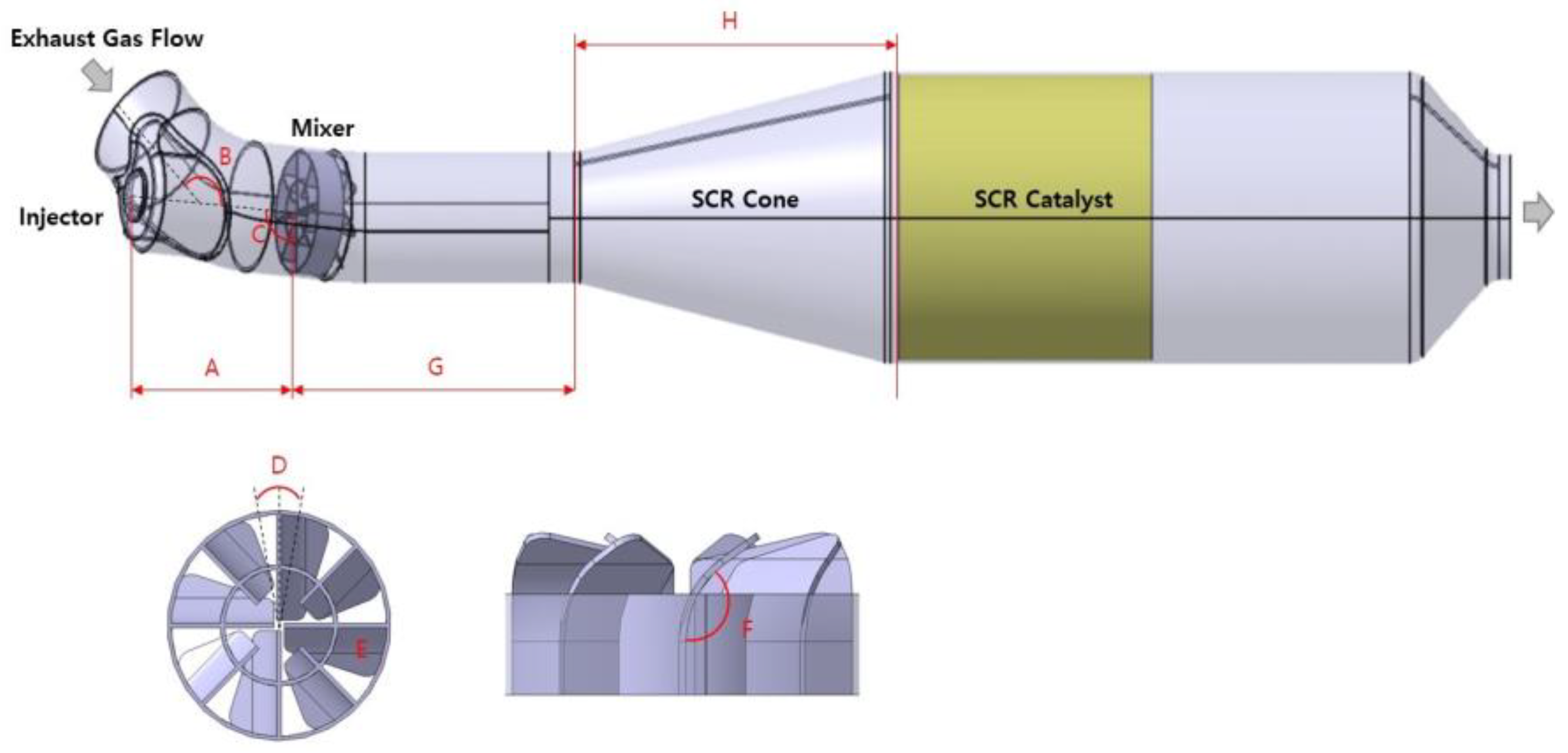

| No. | Major Design Parameters | Unit |
|---|---|---|
| 1 | A: Distance between the Urea Injector and Mixer | mm |
| 2 | B: Inflow Angle of the Exhaust Gas | deg. |
| 3 | C: Angle of the Urea Injector and Mixer | deg. |
| 4 | D: Mounting Angle of the Mixer | deg. |
| 5 | E: Number of Mixer Blades | No. |
| 6 | F: Bending Angle of Mixer Blades | deg. |
| 7 | G: Distance between the Mixer and SCR Cone | mm |
| 8 | H: Length of the SCR Cone | mm |
| No. | Major Design Parameters | Unit | Design Parameter Sets | ||
|---|---|---|---|---|---|
| Initial | Upper Limit | Lower Limit | |||
| 1 | A: Distance between the Urea Injector and Mixer | mm | 85 | 95 | 75 |
| 2 | B: Inflow Angle of the Exhaust Gas | deg. | 109 | 114 | 104 |
| 3 | C: Angle of the Urea Injector and Mixer | deg. | 110 | 115 | 105 |
| 4 | D: Mounting Angle of the Mixer | deg. | 0 | 10 | −10 |
| 5 | E: Number of Mixer Blades | No. | 6 | 8 | 4 |
| 6 | F: Bending Angle of Mixer Blades | deg. | 120 | 125 | 115 |
| 7 | G: Distance between the Mixer and SCR Cone | mm | 167 | 187 | 147 |
| 8 | H: Length of the SCR Cone | mm | 166 | 186 | 146 |
| Ranking No. | Algorithm | Plot | Norm. RMSE(%) | RMSE | Max. Abs. Error |
|---|---|---|---|---|---|
| 1 | KRG | 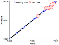 | 28.5% | 0.004 | 0.008 |
| 2 | EDT | 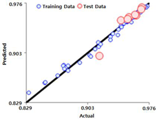 | 57.0% | 0.008 | 0.020 |
| 3 | RBFi | 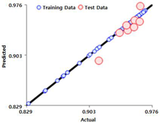 | 82.5% | 0.011 | 0.021 |
| No. | Major Design Parameters | Unit | Value | NH3 UI | |
|---|---|---|---|---|---|
| Prediction | CFD | ||||
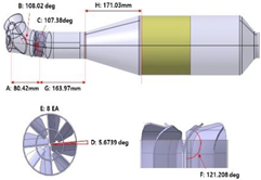
| 1 | A: Distance between the Urea Injector and Mixer | mm | 80.42 | 0.97461 | 0.97293 |
| 2 | B: Inflow Angle of the Exhaust Gas | deg. | 107.38 | ||
| 3 | C: Angle of the Urea Injector and Mixer | deg. | 108.02 | ||
| 4 | D: Mounting Angle of the Mixer | deg. | 5.67 | ||
| 5 | E: Number of Mixer Blades | No. | 8 | ||
| 6 | F: Bending Angle of Mixer Blades | deg. | 121.21 | ||
| 7 | G: Distance between the Mixer and SCR Cone | mm | 163.97 | ||
| 8 | H: Length of the SCR Cone | mm | 171.03 | ||
| Matching Rate (%) | 99.83 | ||||
| No. | Major Design Parameters | Contribution Analysis [%] |
|---|---|---|
| 1 | A: Distance between the Urea Injector and Mixer | 4 |
| 2 | B: Inflow Angle of the Exhaust Gas | 7 |
| 3 | C: Angle of the Urea Injector and Mixer | 0 |
| 4 | D: Mounting Angle of the Mixer | 19 |
| 5 | E: Number of Mixer Blades | 100 |
| 6 | F: Bending Angle of Mixer Blades | 22 |
| 7 | G: Distance between the Mixer and SCR Cone | 0 |
| 8 | H: Length of the SCR Cone | 3 |
| Base Model | DOE Optimization | Metamodel Optimization |
|---|---|---|
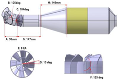 | 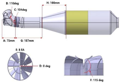 |  |
| NH3 UI: 0.959639 | NH3 UI: 0.973499 | NH3 UI: 0.972931 |
| Classification | Base Model | DOE Optimization | Metamodel Optimization |
|---|---|---|---|
| Results of Optimization | 0.959639 | 0.9734991 (1.44%↑) | 0.972931(1.38%↑) |
| Data Quantity | 1 | 27 | 87 |
| Contribution | N/A | N/A | E > F > D |
| Prediction | N/A | N/A | Predictable |
Disclaimer/Publisher’s Note: The statements, opinions and data contained in all publications are solely those of the individual author(s) and contributor(s) and not of MDPI and/or the editor(s). MDPI and/or the editor(s) disclaim responsibility for any injury to people or property resulting from any ideas, methods, instructions or products referred to in the content. |
© 2023 by the authors. Licensee MDPI, Basel, Switzerland. This article is an open access article distributed under the terms and conditions of the Creative Commons Attribution (CC BY) license (https://creativecommons.org/licenses/by/4.0/).
Share and Cite
Kim, S.; Park, Y.; Yoo, S.; Lee, S.; Chanda, U.K.; Cho, W.; Lim, O. Optimization of the Uniformity Index Performance in the Selective Catalytic Reduction System Using a Metamodel. Sustainability 2023, 15, 13803. https://doi.org/10.3390/su151813803
Kim S, Park Y, Yoo S, Lee S, Chanda UK, Cho W, Lim O. Optimization of the Uniformity Index Performance in the Selective Catalytic Reduction System Using a Metamodel. Sustainability. 2023; 15(18):13803. https://doi.org/10.3390/su151813803
Chicago/Turabian StyleKim, Sunghun, Youngjin Park, Seungbeom Yoo, Sejun Lee, Uttam Kumar Chanda, Wonjun Cho, and Ocktaeck Lim. 2023. "Optimization of the Uniformity Index Performance in the Selective Catalytic Reduction System Using a Metamodel" Sustainability 15, no. 18: 13803. https://doi.org/10.3390/su151813803
APA StyleKim, S., Park, Y., Yoo, S., Lee, S., Chanda, U. K., Cho, W., & Lim, O. (2023). Optimization of the Uniformity Index Performance in the Selective Catalytic Reduction System Using a Metamodel. Sustainability, 15(18), 13803. https://doi.org/10.3390/su151813803