Comparative Evaluation and Multi-Objective Optimization of Cold Plate Designed for the Lithium-Ion Battery Pack of an Electrical Pickup by Using Taguchi–Grey Relational Analysis

Abstract

It is aimed to minimize carbon emissions and the spread of electric vehicles is supported for a more sustainable future. To increase the safety and life of these vehicles, cooling systems are added and developed to their energy storage systems. The aim of this study is to design and optimize the cooling plate for the lithium-ion battery pack used in a lightweight commercial electrical vehicle. Multi-objective optimization using Taguchi–grey relational analysis was performed by considering maximum temperature, the standard deviation of temperature, and pressure drop for the design of the cold plate. Channel number, channel height, and mass flow rate values were determined as parameters to be examined, and three different levels were selected for each parameter. Analysis was performed using water and 25% and 50% ethylene glycol–water solutions, which can work under sub-zero environmental conditions, employed as cooling fluid. It is shown that increasing the ethylene glycol ratio in the coolant allows it to work in colder environmental conditions, it is relatively worsening thermal performances in the cold plate applications. A new empirical correlation is proposed to predict the Nusselt number for the three coolants under all geometric and operating conditions considered in this study. Statistical analysis shows that the number of channels is the most effective parameter for the relatively low and homogenous temperature distribution on the cold plate surface. A sensitivity analysis was performed for Reynolds number ranges from 2500 to 15,000 using the optimum configurations of the three coolant fluids. It is shown that the same cooling effects could be obtained by using 1.56 times and 2.66 times more mass flow rates for 25% and 50% ethylene glycol–water solutions, respectively, compared to the water. However, rising mass flow rates result in a significant increase in the required pumping power.

1. Introduction

The development of technology, the increase in the population, and the ability of societies to reach their needs more easily and cheaply have increased the demand and consumption volume in the global market. With the gradual increase in consumption, the burden on the transportation sector has increased and has led to the use of more transportation vehicles [1]. However, this increase affects the demand to energy and the carbon dioxide emission to a significant extent [2,3,4]. When the carbon emissions related to the sectors are examined, it is seen that the carbon emission in the transportation sector constitutes approximately one fourth of the total emissions [5]. Various measures are taken by the states in order to minimize these emissions caused by global warming and to bring the amount of CO₂ to its pre-industrial value [6,7]. For net zero emission, which is aimed for in light of these actions, electric vehicles and their systems have started to be developed [8,9]. Lithium-ion batteries are very common for energy storage systems, which is one of the most important among them. Having a high energy density and low self-discharge, being able to charge fast, and being able to easily design a pack according to needs are among the main reasons for its frequent use [10,11] Although it has many advantages, there are also points to be considered during its production and use. Since this stored energy has a high energy density and contains flammable solvents, more safety precautions should be taken compared to other batteries [12,13]. Li-ion batteries are extremely temperature-sensitive in terms of their performance, life, and safety. It is known that for almost all cell materials, the performance and stability of Li-ion batteries are decreased at the anomalous temperature range [14]. Because there are so many different electrode materials and electrolyte combinations used in commercial batteries, it is challenging to create a comprehensive and coherent process that improves the performance and safety of Li-ion batteries. For this reason, in most cases, the battery thermal management system (BTMS) should be used in order for the battery to work within the specified temperature ranges and to have a uniform temperature distribution between the cells [15].

Battery cooling systems can generally be examined in two categories as active systems and passive systems. In passive systems, the heat dissipation occurs by conduction, natural convection, and/or radiation, while in active systems, this is done by means of a pump or fan using a refrigerant. Phase change materials (PCM) and heat pipes are commonly employed in passive systems [16,17]. Since phase change materials (PCM) can absorb and release a large amount of heat, they can maintain batteries between certain temperatures. As they can vary according to the application, they are generally used for liquid–solid transitions [18]. As the temperature increases, the PCM absorbs the heat and changes from solid to liquid state; in the opposite case, heat is given to the environment by the exothermic process, and it returns to the solid state [19]. Aslan et al. [20] investigated the effect of graphene additives on PCM with three different mechanisms to increase the low thermal conductivity of PCM. They observed that the first and third designs did not have a noticeable contribution to heat transfer, but the second design supplemented with PCM–graphene significantly improved the heat transfer and provided faster cooling. A novel hybrid battery thermal management system with a nickel–titanium shape memory alloy actuated smart wire and PCM with expanded graphite was proposed by Joula et al. [21]. They stated that the suggested design easily prevents overheating the battery. Since there are no additional parts in passive systems, they are lighter than active ones, but they are not suitable for use in situations where effective cooling is required. Air cooling can be used in both passive systems using air velocity and in active systems with the help of a fan [22,23,24]. The fundamental advantage of air cooling systems over liquid coolant systems is their simplicity, electrical safety, and cost [16,25]. However, the cooling capacity of these systems is very limited due to the lower heat transfer coefficient of air and it is difficult to ensure uniformity throughout the battery pack [26,27,28,29].

Systems with liquid cooling are divided into direct and indirect methods. In direct cooling, the batteries are immersed in the dielectric refrigerant. Although its design is simple and it is a very effective cooling method, it is not common due to a possible leakage problem. While indirect cooling can be in the form of matrix, fins, or plates depending on the design of the pack and different types of refrigerants can also be used depending on the material [30]. A comparative study based on air cooling, direct liquid cooling, indirect liquid cooling, and fin cooling for lithium ion battery cells was performed by Chen et al. [31]. They concluded that indirect liquid cooling is a more practical form than direct liquid cooling though it has slightly lower cooling performance.

As summarized in the literature given above, despite being more complex, heavy, and expensive, indirect liquid cooling systems provide superior performance and easier management with lesser configurable space occupancy in BTMS applications. Among indirect liquid cooling-based BTMS, cooling plate with channels is the most frequently used one [32]. Researchers have carried out investigations using different channel geometries. Smith et al. [14] analyzed and compared three different plate designs at different ambient temperatures, different fluid temperatures, and different mass flow rates. As a result of the analysis, they stated that the U-shape plate came to the fore when thermal performance, energy consumption, and vehicle integration were taken into account. They also added that the heat transfer increased with the increase of the contact surface. Finally, they reported that the gradients of each device on a single cell were similar, and the largest gradients were observed in the region of the coolant inlet. In another study, Li et al. [33] carried out a numerical analysis of cooling plate geometries with different structures and discussed the results. After a series of simulations, they stated that the plate with the convex structure provided the optimum cooling among the other three configurations. In addition, they added that as the mass flow rate increases, the heat transfer also increases. Benabdelaziz et al. [34] developed a cooling system for an electric vehicle battery and analyzed alternative cooling systems. As a result of the analysis, they observed that the second design kept the maximum temperature under control and reduced the temperature gradients due to the contact surface area.

Those working on these systems examine the effects of not only geometry but also different parameters on heat transfer. Mei et al. [35] investigated the effects of different discharge rates, different coolant flow rates, and different inlet temperatures on the heat transfer and uniformity of a lithium-ion battery in flat heat pipes placed between rectangular cells. According to the findings, they stated that as the mass flow rate increases and the inlet temperature decreases, the maximum temperature is significantly reduced. In addition, they reported that with the increase of the discharge rate, the maximum temperature of the battery, the temperature in the battery is different and the average temperature of each cell gradually decreases. Lan et al. [36] designed an aluminum mini channel integrated into a single prismatic lithium-ion cell under different discharge rates. The performances of these battery management systems were investigated using different flow rates and configurations. At the end of the study, it was noted that as the discharge value increased, the mass flow value required to keep the temperature at a certain level increased and the required pump power increased. In another study, Zhao et al. [37] analyzed a mini-channel liquid cooling plate for lithium-ion battery with cylindrical geometry. In the study, the effect of the number of channels, mass flow, flow direction, and inlet dimensions on heat transfer was emphasized. In the findings, it has been stated that the liquid-cooled system for the examined battery provides advantages over convection cooling only when the number of channels is more than eight, the ability to control a temperature is limited with the increase in mass flow rate, and the heat dissipation capacity is related to the inlet dimensions when the inlet mass flow rate remains constant.

Another method used to improve battery management systems is to optimize the existing system using various optimization techniques including statistical analysis methods such as Taguchi, Latin hypercube sampling (LHS), ANOVA, and grey relational analysis (GRA) [38,39,40]. For example, Mo et al. [41] optimized the traditional cooling plate design with the topology optimization method. At the end of the analysis, velocity, pressure, and temperature results for optimized and traditional cooling plates were compared. In addition, the effects of mass flow rate and inlet temperature on performance were included in the analysis. They noted that the pressure drop value on the topology-optimized cooling plate decreased by 47.9% and the maximum temperature value decreased by 2.3 °C. Another study on this subject was conducted by Ye et al. [42]. In their study, they used an orthogonal matrix for the optimization of the cooling system they designed. The parameters they determined for the study are the battery gap, the cross-section size, and the number of the cooling channel. The results showed that the optimized cooling plate reduced the maximum and minimum temperatures by 9.5%, while the pressure drop was reduced by 16.88%. Egab and Oudah [43] have used dimples to increase heat transfer. They used circular, elliptic, and cylindrical geometries to achieve effective cooling. The working fluid was chosen as air, and they adopted laminar flow. At the end of the study, it was seen that cylindrical dimples provide one and a half times more heat transfer than the geometry with no dimples, and the shapes of these geometries have a slight effect on the thermal performance of the battery. The study by Ling et al. [44] can be shown as an example of a study in which the cooling performance is examined using the Taguchi optimization method. In the study, the Taguchi method and digital heat transfer model were used to minimize the weight and volume of the thermal management system. At the end of the optimization, it was noted that the hybrid system studied had higher efficiency and lighter weight than conventional liquid cooling systems. Naqiuddin et al. [45] worked on a segmented microchannel to increase the thermal performance of the cooler with a flat channel. Jiaqiang et al. [46] investigated the orthogonal matrix with L16 experimental setup to examine the effect of four different parameters they determined on a Li-ion battery with liquid cooling, and they found that the number of pipes is the most effective parameter, but the pipe height has the most effect on the cooling performance. Kılıç and Şentürk [47] investigated the case where the heat transfer performance is the highest and the required pump power is the lowest by using the multi-response Taguchi method in their study on mini-channel cooler blocks with liquid cooling.

The efficiency and performance of the cooling system are greatly influenced by the operational and design parameters, such as working fluid, flow geometry, mass flow rate, height, and width of the channels. Researchers have published numerous optimization studies using various approaches in the literature. Yet, there has not been thorough research that examines all these variables and uses statistics to calculate their relative contributions to the system’s performance. As a result, the goal of this study is to investigate the parameters that have the greatest impact on the values of the cooling plate performance and to rank these parameters according to their significance using the Taguchi–grey relational analysis and ANOVA methodologies. Moreover, several statistical analysis techniques are used to establish the ideal working conditions, and the results are compared. In view of these, the main contribution of the present study can be stated as follows. Firstly, a new multi-channel liquid cooling plate was designed based on the lithium-ion battery pack in the lightweight commercial vehicle manufactured by Goupil Industrie. Secondly, a one-dimensional battery model was created and validated for the constant heat flux limit condition required during the analysis, and the required value was obtained. Thirdly, a multi-objective optimization procedure by means of the Taguchi–grey relational analysis method was performed to optimize the new cooling plate configuration with the objective of minimizing the pressure drop of the fluid flow, the battery pack surface temperature, and its variation, by using controllable factors, including working fluid, the mass flow rate, the number of channels, and the height and width of the channels. Plain water was chosen as the coolant in most similar studies. However, water is not suitable for operation at low temperatures below zero. In this study, 25% (EGW 25) and 50% (EGW 50) ethylene glycol–water solutions that can operate under sub-zero ambient temperature conditions were also analyzed and their performances were compared and evaluated. For the multi-objective optimization, Taguchi and ANOVA statistical analysis methods were used to obtain the control factors’ effect degrees and ratios.

2. Materials and Methods

2.1. Testing and One-Dimensional Generic Model of the Battery

During the charge and discharge processes, heat generation occurs throughout the battery cell due to the chemical reactions, polarization, and Joule heat value [48]. However, expressing this as a constant value is not sufficient since it depends on the charging or discharging processes. AMESIM software [49] was used to find the heat produced by the battery. A one-dimensional (1D) model of the battery and a generic thermal model was created and analyzed from 0% SOC (State of Charge) to 100% SOC.

The generic battery model is as shown in Figure 1. The sub-element numbered 1 represents the battery. Due to the data needed, a generic model is preferred instead of the cell-based model. A battery pre-sizing tool was used to observe the temperature change. It is the element used for the current input shown with 2. The thermal model of the battery is shown with 3. To simplify the model, only convection is modeled. Finally, the sub-element shown with 4 indicates battery and cell materials.

The energy equation for a cylindrical battery cell [15,50] can be written as:

$${\rho }_b{c}_{pb}\frac{dT}{dt}=k_r \frac{1}{r} \frac{d}{dr} \left(r \frac{dT}{dr}\right)+k_{\phi } \frac{1}{r^2} \frac{d^{2}T}{d{\phi }^2}+k_z \frac{d^{2}T}{d{z}^2}+Q_g$$

(1)

where $Q_g$ represents the heat generation rate in the battery. It can be calculated as given in Equation (2) [51].

$$Q_g=I \left(E-E_{oc}\right)+I \left[T \frac{d{E}_{oc}}{dT}\right]$$

(2)

where I (A) is the charge/discharge current, E_oc (V) is the open circuit voltage, E (V) is the working voltage, T (K) is the temperature, dE_oc/dT is the entropy coefficient which depends on the battery state of charge (SOC), battery temperature, and density.

Element number 2 seen in Figure 1 is placed for the current input. The elements indicated with 3 are the heat transfer model created to obtain the average temperature outputs required for the comparison of the temperature results. Finally, the fourth elements are used to define the material required to calculate the heat transfer. Considering the ease of design and the data needed, a general model was used instead of the cell-based model. The internal resistance and open circuit voltage values obtained from the manufacturer are the values obtained at a single ambient temperature. However, this makes it impossible to perform analyses at different ambient temperatures. For this reason, the battery model was created based on real data and using the battery pre-sizing tool in AMESIM [49]. The mentioned battery pre-sizing tool is as shown in Figure 2. The data of the battery to be modeled were entered in the area marked as A and the outputs in the section indicated with B were calculated and four different graphs based on the temperatures in section C were created by AMESIM.

Parallel to the AMESIM modeling, the charging test was performed in reality by using a test bench. Thermal sensors are connected to the battery and the battery is expected to charge from 0% to 100% SOC. Although the ambient temperature is accepted as 25 °C, the mentioned test was carried out in an open environment. For this reason, the outdoor temperature could not be controlled and its effect on the battery could not be fully investigated during the test.

In Figure 3, the potential graphics of the current batteries under charging tests performed in AMESIM and the test bench are given. Although there are large differences (about 6%) at the beginning of the period, the differences decrease to less than 3% in the rest of the testing period. It was observed that both graphs showed similar behavior.

The average temperatures obtained from the two tests are given in

Table 1. Comparison of temperature outputs.

	AMESIM	Measured	Difference (%)
Average Battery Temperature (°C)	30.31	33.19	8.7

. One of the reasons for the current deviation in the mean temperature outputs is that the battery modeled in AMESIM is constructed using a pre-sizing tool in certain approaches. This tool applies real data to mathematical models and obtains graphs indicated with C in Figure 3 for certain temperature ranges. Due to this approach, a certain deviation is expected. Another reason is that, as mentioned before, the environment was not isolated for the test-bench. Therefore, it can be assumed that the test is affected by the ambient temperature. Considering these conditions, the validation of the 1D model created was approved and used for further tests.

The value to be used as a limit condition for the computational fluid dynamics (CFD) analysis was determined by the AMESIM model. As current input, 200 A was determined and a heat flux value for 50% SOC condition was calculated with a post processing section. The heat flux value obtained as a result of the AMESIM analysis is as seen in Figure 4.

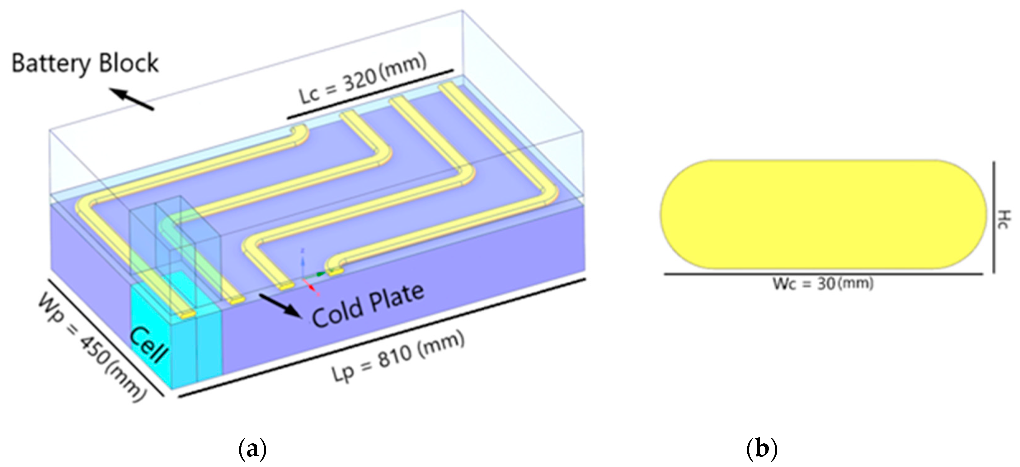
2.2. Physical Model and Used Materials of Cooling Plate

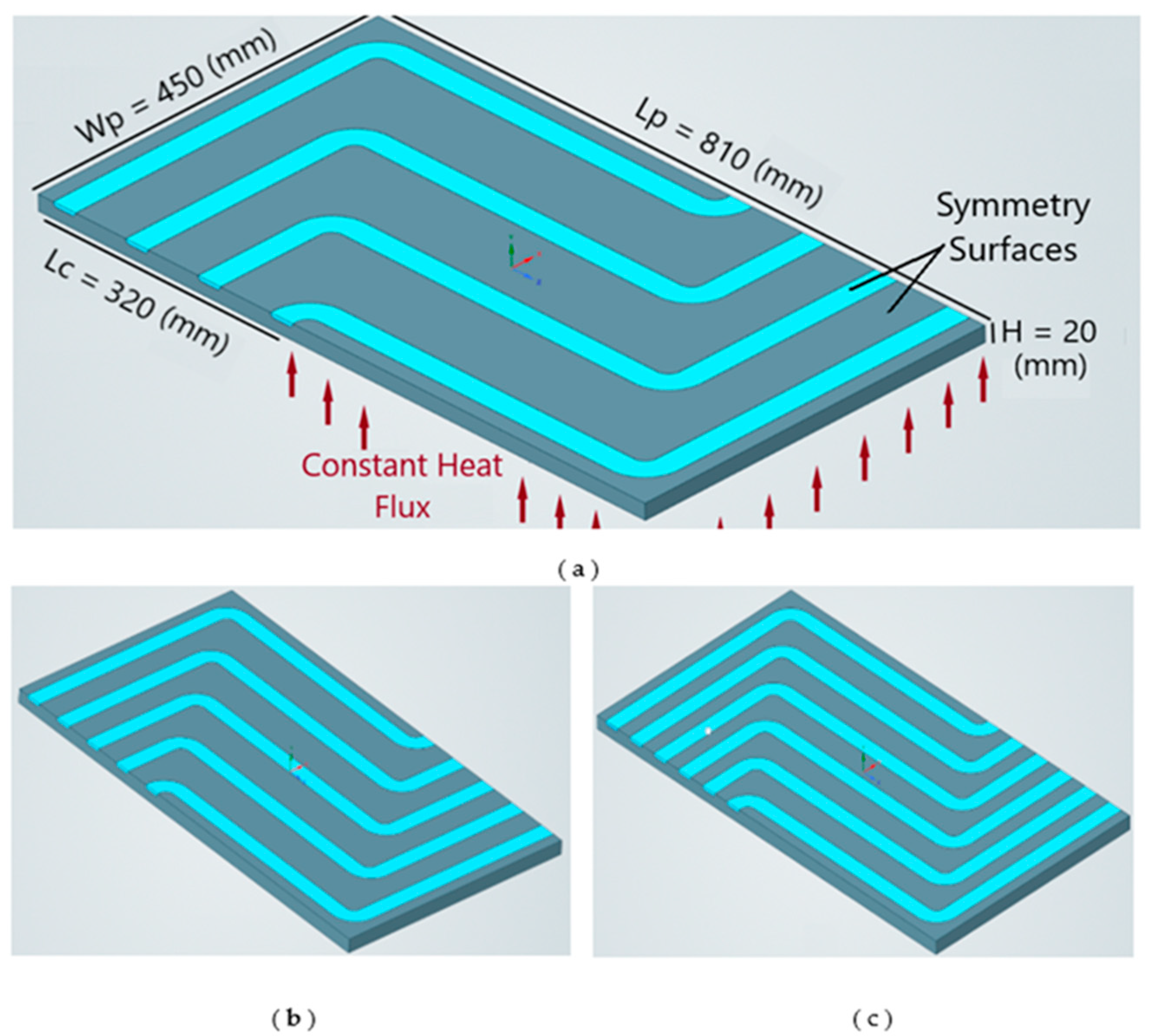
While designing the cooling plate examined in the study, the dimensions of the battery used in the GOUPIL G6 lightweight commercial electrical vehicle were used as a base, and the battery measured 450 mm × 810 mm. Therefore, the heat sink was built to be the same size as the battery pack as shown in Figure 5.

Since the geometry is symmetrical, only half of it was modeled; a symmetry boundary condition was defined for the upper part of the cooling plate and a constant heat flux of 3020 W/m² was applied to the lower part of the cooling plate. However, since the heat produced by the battery was not constant, the generic thermal model of the battery was created using the AMESIM software and optimized by comparing it with the real-time experiment. As a result, the constant current value was given to the model and the constant heat flux value used in the analysis was determined.

The cold plate geometries with three different channel numbers used in the study are shown in Figure 6 and L_p, W_p, H_p represent the length, depth, and height of the cooler, respectively. L_c is the total length of the area occupied by the duct, and all the ducts are located in a fixed area, the length of the area is 320 mm. The distance of the area from the outer surfaces of the plate was kept constant at 15 mm and the plate thickness at 20 mm.

The width of the channels was kept constant at 30 mm; only the height was increased, and the channel heights used were 10 mm, 12 mm, and 14 mm, respectively. Four, five, and six channels were used in the analyzed geometries.

For full development conditions of the flow, the channels were extended out of the plate as previously mentioned. The extended channel length is called the hydrodynamic inlet length (L_h) [52]. Hydrodynamic inlet length in turbulent flow:

$${10D_h \le L}_h \le 60D_h$$

(3)

The hydraulic diameter is denoted by D_h in the given equations and it is the expression used instead of the diameter if the cross-section of the channel through which the fluid passes is a shape other than a circle. The hydraulic diameter is the ratio of the cross-sectional area (A) of flow to the wetted perimeter (P). Since the channel resembles an ellipse in this study, the hydraulic diameter calculation is given below Equation (4).

$$D_h=\frac{4A}{P}=\frac{\pi {H_c}^2+4H_c{(W}_c-H_c)}{\pi H_c+2(W_c-H_c)}$$

(4)

The number of channels (NOC), channel height (H_c), and fluid flow rate (M), which are the factors whose effects will be investigated in order to examine the pressure drop in the cooling block, the maximum temperature on the surface in contact with the battery, and the standard deviation of the temperature on the same surface in order to ensure temperature homogeneity are given in

Table 2. Factors and levels whose effects were investigated.

Parameters	Coolant	(NOC) Number of Channels	(Hc) Channel Height (mm)	(M) Mass Flow Rate (kg/s)
Level 1	Water	4	10	0.8
Level 2	EGW 25	5	12	1
Level 3	EGW 50	6	14	1.2

. The factors given to ensure the lowest thermal resistance, temperature homogeneity, and pressure drop were investigated using Taguchi’s experimental design. In order to observe the effect of different refrigerants in the best way, the analyses were repeated for each fluid, keeping the other three parameters (factors) independent from the Taguchi matrix. Since the vehicle could work under zero environmental temperature conditions, in addition to water, two other fluid solutions which work under sub-zero conditions were considered. Pure water, the mixtures of water, 25% (EGW 25) and 50% (EGW 50) ethylene glycol–water solutions were used as the coolant fluid. The cold plate material was chosen as aluminum. The thermo-physical properties of refrigerant and solid materials are given in

Table 3. Thermophysical properties of fluid and solid materials [53].

Specifications	Coolant Fluids			Material of the Plate
	Water	EGW 25	EGW 50	Aluminum
Density ($\rho$) (kg/m3)	998.2	1028	1061	2719
Specific heat ($c_p$) (J/kg K)	4182	3827	3348	871
Heat transfer coefficient (k) (W/mK)	0.6	0.493	0.3935	202.4
Viscosity (µ) (Ns/m²)	0.001003	0.001564	0.002974
Prandtl Number (Pr)	6.99	12.14	23.30
Freezing temperature (°C)	0	−10	−36

, which were obtained by using Engineering Equation Solver (EES, V.11) internal libraries [53]. It can be seen that the freezing temperatures for water, EGW 25, and EGW 50 are 0, −10, and −36 degrees Celsius, respectively.

For the optimization of the cooling plate used in the study, the orthogonal arrays developed by Taguchi were used and the calculation was made with the noise ratio (S/N—signal/noise) analysis.

Table 4. Taguchi orthogonal array for turbulent flow design.

Factors/ Levels	NOC	Hc	M
1	4	10	0.8
2	4	12	1
3	4	14	1.2
4	5	10	1
5	5	12	1.2
6	5	14	0.8
7	6	10	1.2
8	6	12	0.8
9	6	14	1

shows the level combinations created according to the Taguchi L9 (3³) statistical design used in this study and used in CFD analysis.

2.3. CFD Model

The combined three-dimensional model of the solid and fluid volumes in the cold-plate is given in Figure 6. The finite volume method is employed to perform the computation to solve the flow field and to obtain conjugate heat transfer in both solid and fluid regions [54]. Numerical computations to solve governing equations as conservation of mass, momentum, and energy equations were realized by using ANSYS Fluent (Release 19.2). The SIMPLE (Semi-Implicit Method for Pressure Linked Equations) algorithm was used for the coupling of pressure–velocity in the fluid region [55]. Detailed information and descriptions of the numerical methods can be found in Ref. [56]. The conservation equations used in numerical analysis are given below.

Continuity equation:

$$\frac{\partial \left({\rho u}_i\right)}{\partial x_i}=0$$

(5)

Momentum conservation equations in x, y, and z directions:

$$\frac{\partial }{\partial x_i}\left(\rho u_i{u}_j\right)=-\frac{\partial p}{\partial x_i}+\frac{\partial }{\partial x_i}\left[\left(\mu + {\mu }_t\right)\frac{\partial u_j}{\partial x_i}\right]+S_c$$

(6)

Energy conservation equation:

$$\frac{\partial }{\partial x_i}\left(\rho u_i{c}_{p}T\right)=\frac{\partial }{\partial x_i}\left[k_f\frac{\partial T}{\partial x_i}\right]+S_c$$

(7)

where x_i (m) is the coordinate component, 𝜌 (kg/m³) is the density of the fluid, u_i (m/s) is the velocity component, 𝑐_𝑝 the specific heat of the fluid (J/kg K), µ (Ns/m²) is the dynamic viscosity, µ_t (Ns/m²) is the turbulent viscosity, p is the pressure (Pa), g (m/s²) is the gravitational acceleration where 𝑇 is the temperature (K) and S_c represents the volumetric source terms. Turbulent viscosity was calculated by using the eddy viscosity approach as given in Equation (8):

$${\mu }_t=\rho \frac{k}{\omega }$$

(8)

where k is the turbulence kinetic energy, $\omega$ is the specific dissipation rate. Turbulence properties can be obtained by using the two-equation k − $\omega$ turbulence model as given in Equations (9) and (10) [56,57].

$$\frac{\partial \left(\rho k\right)}{\partial t}+\frac{\partial \left(\rho u_{j}k\right)}{\partial x_j}={\tau }_{ij}\frac{\partial \left(u_i\right)}{\partial x_j}-{\beta }^{*}\rho \omega k+\frac{\partial }{\partial x_j}\left[\left(\mu +{\sigma }_k\frac{\rho k}{\omega }\right)\frac{\partial k}{\partial x_j}\right]$$

(9)

$$\frac{\partial \left(\rho \omega \right)}{\partial t}+\frac{\partial \left(\rho u_j\omega \right)}{\partial x_j}=\frac{\gamma \omega }{k}{\tau }_{ij}\frac{\partial \left(u_i\right)}{\partial x_j}-\beta \rho {\omega }^2+\frac{\partial }{\partial x_j}\left[\left(\mu +{\sigma }_{\omega }\frac{\rho k}{\omega }\right)\frac{\partial \omega }{\partial x_j}\right]$$

(10)

where model constants were taken as: γ = 0.52, β = 0.072, β* = 0.09, σ_k = 0.5, and σ_ω = 0.5.

Assumptions and boundary conditions were applied in numerical CFD analysis as follows:

• The flow is steady-state, three-dimensional, and turbulent in a continuous regime.
• The properties of the solid and the fluid do not change with temperature.
• Since the working fluid is liquid, the variation of the density can be ignored. Hence, fluid can be acceptable as incompressible.
• No-slip boundary condition was used for solid–fluid boundary surfaces.
• Since the surface area of the side walls are smaller compared to the heat flux surface (horizontal surface), the adiabatic boundary condition was applied to the side walls of the solid region (cold plate).
• Channel inlets and outlets were extended by 300 mm, which is ten times the channel width. Then, homogeneous velocity distribution was taken at the extended channel entrance.
• Pressure boundary condition at the channel outlet was applied.
• Coupled interface definitions were made on these common surfaces between the cold plate and the channels, and mesh interfaces were created fluently so that the software could solve the heat transfer in these regions.
• Only the energy equation was solved in the solid part of the cold plate geometry.
• Since the geometry and conditions were symmetric with respect to the middle horizontal plane of the cold plate, the symmetry conditions were applied at those surfaces.
• As it is discussed in Section 2.2, constant heat flux boundary condition was applied at the bottom surface of the cold plate.
• The normalized residuals of the governing equations were considered for the convergence criteria. During the computations, it was accepted that the numerical simulation was converged when the normalized residuals of the continuity, momentum, and turbulence equations were less than 10⁻⁵ and the energy equation was less than 10⁻⁷.

2.4. Validation and Mesh Independence Study

Since the geometries to be used in the study cannot be validated experimentally, we aimed to provide validation of the methods to be used during the analysis by considering a similar study. For the validation, the optimization of the cold plate used in electric vehicle batteries studied by Jarrett and Kim [58] was chosen. The fluid that passed through the fluid domain was a water–50% ethylene glycol mixture. The outer dimensions of the geometry were 1 mm × 160 mm × 200 mm as specified in the paper. The geometry to be analyzed was symmetrical, so the thickness was reduced to 0.5 mm and only half of the geometry was created in 3D. A total of 243,971 elements were used and 240,874 of them were in the fluid domain. The inlet boundary condition was set as mass–flow–inlet and 0.0005 kg/s value was given as input. For the heat flux boundary condition, 500 W/m² was applied, similar to the reference study. Three different calculated parameters were considered for the validation. These were the mean temperature on the heat flux surface, T_mean, the standard deviation of the temperature on the heat flux surface, T_σ, and the pressure drop, ΔP, between the inlet and the outlet.

Table 5. Comparison of the present results with the data of the reference study.

Parameter	Present Calculation	Data of Reference [58]	% Difference
Tmean (K)	306.12	306.09	0
Tσ (K)	2.54	2.51	1.2
ΔP (Pa)	3007	2948	2

shows the comparison of the present computation and the results given in the reference study [58]. It can be seen that the results show very good agreement with the reference ones. Therefore, the present model was assumed as validated.

Results from the analysis vary up to a certain number of items. Increasing the number of elements after this limit does not make the solution more accurate, but also increases the solution time and makes the analysis more costly [59]. This limit of the element number value, where the variation is negligible and almost unobservable, is used for the mesh-independent results. For the mesh dependency test, six different mesh structures with the elements numbers between 1.6 × 10⁶ and 5 × 10⁶ were created and analyzed for turbulent flow with a mass flow rate of 0.2 kg/s, for geometry with four channels and a height of 10 mm. Figure 7 shows the mesh structure used in the CFD analysis. Tetrahedral elements were used in the mesh structure. Inflation layers were added in order to condense the mesh structure on the channel surfaces and to provide better resolution of the flow.

The maximum temperature on the cold plate surface and the pressure drop between the inlet and the outlet were chosen as the evaluation criteria. Figure 8 shows the comparison of Tmax and ΔP values obtained from the calculations using different mesh element numbers between 1,500,000 to 5,000,000. It was observed that there was not much change after the 2,200,000 elements in the mesh. Therefore, it was assumed that the mesh independent analysis could be performed by using about 2,000,000 mesh elements. Then, the main analyses were carried out according to this mesh structure.

2.5. Parameters Used in the Evaluation of the CFD Analysis

In the analyses, the maximum temperature of the surface for which the constant heat flux was defined, the standard deviation of the temperature on this surface, and the pressure drop along the channel were taken as the result parameters to calculate the thermal resistance, temperature homogeneity, and pump power, respectively. Thermal resistance (Equation (10)) is inversely proportional to the heat transfer coefficient of the material in the solid material and the heat transfer coefficient on the fluid side [29]. The heat transfer coefficient is related to the channel geometry, mass flow rate, and the flow characteristics. Calculation of thermal resistance is as shown below:

$$R=\frac{T_{max}-T_{in}}{qA}$$

(11)

where R represents the thermal resistance (K/W), q represents the heat flux applied to the base (W/m²), and A represents the total surface area to which the heat flux is applied. Considering Equation (11), thermal resistance decreases when maximum temperature approaches the coolant inlet temperature. Therefore, it must be considered in the design and optimization of the cold plate.

In light of the calculated pressure drops, a suitable pump selection should be made according to each case. The required pump power is calculated as shown below:

$$W_p=\dot{V} ∆P$$

(12)

where $\dot{V}$ represents the volumetric flow rate (m³/s) and ΔP the pressure drop (Pa). Since the total mass flow rate, M (kg/s), is known, it is possible to calculate the volumetric flow rate as in Equation (13):

$$\dot{V}=\frac{M}{\rho }$$

(13)

It should be noted that the pressure drop must be as small as possible for an energy-efficient cooling process. Therefore, the pressure drop is another important parameter that must be considered in the design and optimization of the cold plate. These show that multi-objective optimization is an important issue for the design of the cold plate.

The Reynolds number (Equation (14)), denoted by Re, is the dimensionless number representing the ratio of inertial forces to viscous forces in the flow, and indicates that the flow is in the turbulent regime [52]. The Reynolds number is defined as given in Equation (14).

$$Re=\frac{u{D}_h\rho }{\mu }$$

(14)

Table 6. Reynolds numbers and hydraulic diameter calculated according to the Taguchi orthogonal array matrix.

			Reynolds Number
Levels	Dh	M	Water	EGW 25	EGW 50
1	0.0156	0.8	11,168.53	7162.43	3766.66
2	0.0179	1	13,528.17	8675.68	4562.46
3	0.0199	1.2	15,746.01	10,097.98	5310.44
4	0.0156	1	11,168.53	7162.43	3766.66
5	0.0179	1.2	12,987.05	8328.65	4379.96
6	0.0199	0.8	8397.87	5385.59	2832.23
7	0.0156	1.2	11,168.53	7162.43	3766.66
8	0.0179	0.8	7215.03	4627.03	2433.31
9	0.0199	1	8747.78	5609.99	2950.24

shows the Reynolds numbers for the cases considered in this study. After calculating the mass flow rate of a single channel from the mass flow entering the entire block (Equation (15)), the average velocity value of the fluid is reached (Equation (16)).

$${\dot{m}}_k=\frac{M}{N}$$

(15)

$$u=\frac{{\dot{m}}_k}{\rho A_k}$$

(16)

In the equations given here, M (kg/s) is the total mass flow rate to the cold plate; ${\dot{m}}_k$ is the flow rate through a single channel; N is the number of channels; and A_k is the cross-sectional area of the single channel (m²).

2.6. Taguchi-Based Grey Relation Analysis

It has been observed that the experimental design methods, which were first developed by Fischer in the 1930s, were not efficient enough because the number of factors affecting the system increased as the number of experiments increased. Genichi Taguchi made these systems efficient by applying the reduction of variables to experimental designs. Experimental design methods are very efficient optimization approaches when both time and economic conditions are considered. The Taguchi method provides high quality outputs, while ensuring that the solution is obtained with the least number of experiments [60].

After determining the factors and levels to be analyzed, the design needs to be determined. The first data required to determine the matrix order is the total degrees of freedom. The degree of freedom represents the number of parameters determined to reach the optimum result [61].

The data obtained as a result of the experiments are converted into the signal to noise ratio and evaluated. In the S/N ratio, the noise represents the unwanted factors, and the signal represents the desired true value in the obtained values. This ratio is calculated in three different ways as smaller better, larger better, and nominal better according to the target value of the quality value. For the smaller better and the larger better criteria, the S/N ratios can be calculated using Equations (17) and (18), respectively [62].

$$\raisebox{1ex}{$S$}\!\left/ \!\raisebox{-1ex}{$N$}\right.=-10{\log }_{10}\left(\frac{1}{n}\sum _{i=1}^n{y}_i^2 \right)$$

(17)

$$\raisebox{1ex}{$S$}\!\left/ \!\raisebox{-1ex}{$N$}\right.=-10{\log }_{10}\left(\frac{1}{n}\sum _{i=1}^n\frac{1}{y_i^2} \right)$$

(18)

Even if any of the three methods is chosen as the evaluation type, the largest S/N ratio indicates the design with the best experimental result.

The similarities and differences between two elements in a particular system are called the grey relationship, and the grey relation analysis (GRA) is the measurement of the relation between these two elements. If these changes are significant between the two elements, there is a higher relation, and in the opposite case, there is a lower relation [63].

The traditional Taguchi method is used when it comes to optimizing a single performance response of the specified parameter. However, when there is a multi-response optimization problem, hybrid approaches in which multi-criteria decision-making methods are used together with Taguchi should be adopted. Thus, multiple parameters can be converted into a single response. One of these hybrid approaches is Taguchi–grey analysis [64].

The S/N ratios of each response obtained in the GRA method are calculated and the deltas of each parameter are summed. The available data are normalized between 0 and 1 and the grey relational coefficient is calculated from the normalized matrix representing the correlation between the desired and actual experimental data. In the last step, the weight coefficients of each parameter are calculated according to the total delta value and grey relational analysis is performed.

In this study, the objective function “smaller is better”, which is one of three different criteria that maximizes the values of the system, was used because the battery surface temperature and pump power are desired to be low. Equation (19) was used to normalize the output parameters in the GRA method [65].

$$y_i\left(k\right)=\frac{\max x_i^0\left(k\right)-x_i^0\left(k\right)}{\max x_i^0\left(k\right)-\min x_i^0\left(k\right)}$$

(19)

where, $y_i\left(k\right)$ represents the normalization value of the grey relational analysis, and $\max x_i^0\left(k\right)$ and $\min x_i^0\left(k\right)$ are the largest and smallest values of $x_i\left(k\right)$ for the kth response, respectively. In addition, the symbols i and k represent the number of experiments and the number of responses, respectively [66].

After the normalization of the data, the grey correlation coefficient (${\xi }_i$), which relates the ideal and real normalized experimental results, was calculated with the help of Equation (20).

$${\xi }_i\left(k\right)=\frac{{\mathsf{\Delta }}_{min}+\varphi {\mathsf{\Delta }}_{max}}{{\mathsf{\Delta }}_{0i}\left(k\right)+\varphi {\mathsf{\Delta }}_{max}}$$

(20)

$${\mathsf{\Delta }}_{0i}\left(k\right)=‖y_0\left(k\right)-y_i\left(k\right)‖$$

(21)

$${\mathsf{\Delta }}_{max}={max}_{\forall \mathrm{j}\mathrm{ℇ}\mathrm{i}}{max}_{\forall \mathrm{k}}‖y_0\left(k\right)-y_i\left(k\right)‖$$

(22)

$${\mathsf{\Delta }}_{min}= {min}_{\forall \mathrm{j}\mathrm{ℇ}\mathrm{i}}{min}_{\forall \mathrm{k}}‖y_0\left(k\right)-y_i\left(k\right)‖$$

(23)

${\mathsf{\Delta }}_{0i}\left(k\right)$ $\mathrm{i}\mathrm{n} \mathrm{E}\mathrm{q}\mathrm{u}\mathrm{a}\mathrm{t}\mathrm{i}\mathrm{o}\mathrm{n} \left(21\right)$ is the deviation between $y_0\left(k\right)$ and $y_i\left(k\right)$. Equations (22) and (23) can be used to calculate Δ_max and Δ_min, respectively. $\varphi$, which is defined as the discriminant coefficient, was in the range of 0–1 and $\varphi$ was taken as 0.5 [63]. Grey relational degree (γ_i) with normalized weight factor is calculated by Equation (24).

$${\gamma }_i=\frac{1}{n} \sum _{k=1}^n{w}_k{\xi }_i\left(k\right)$$

(24)

In this equation, n is the number of process responses. A high ${\gamma }_i$ designates a strong correlation between $y_0\left(k\right)$ and $y_i\left(k\right)$. ${\gamma }_i$ is used to determine the closeness of the compared serial value to the reference serial value. Therefore, if the two series have the same values, ${\gamma }_i=1$.

In Equation (24), $\sum _{k=1}^n{w}_k=1$, where w_k is the normalized weighting factor for each response. In order to reduce the multi-objective optimization problem to a single equation, the effect ratio of each output parameter on the objective function is expressed with a weight factor and calculated by Equation (25).

$$w_i=\frac{{\sum }_{j=1}^p{Delta}_{i,j}}{\sum _{i=1}^t{\sum }_{j=1}^p{Delta}_{i,j}}$$

(25)

In the equation, $t$ denotes the number of responses, $p$ is the number of parameters, and $Delta$ is the range of S/N.

3. Results and Discussions

3.1. General Evaluations of the Results

The calculated results for the three coolant fluids separately according to the Taguchi orthogonal matrix are given in

Table 7. Obtained results for the Taguchi orthogonal matrix conditions.

Parameters/Arrays	Water				EGW25				EGW50
	Tmax (K)	Tmean (K)	Tσ	∆P (Pa)	Tmax (K)	Tmean (K)	Tσ	∆P (Pa)	Tmax (K)	Tmean (K)	Tσ	∆P (Pa)
L1	305.44	303.36	1.02	1099.20	306.54	304.34	1.10	1229.84	309.30	306.50	1.34	1444.32
L2	305.23	303.19	1.03	1050.27	306.24	304.06	1.10	1185.10	308.80	306.11	1.30	1396.90
L3	305.13	303.07	1.03	1009.82	306.10	303.89	1.10	1140.10	308.36	305.73	1.28	1361.86
L4	303.58	302.37	0.54	1096.83	304.44	303.14	0.60	1227.72	306.65	304.86	0.82	1441.14
L5	303.51	302.28	0.54	978.00	304.30	302.98	0.60	1104.75	306.41	304.67	0.77	1303.57
L6	304.55	303.12	0.63	355.46	305.93	304.23	0.75	398.72	309.07	306.58	1.14	473.66
L7	303.47	301.85	0.36	1109.72	304.07	302.49	0.42	1244.48	305.30	303.94	0.64	1456.62
L8	304.28	302.64	0.45	371.34	305.14	303.65	0.59	412.44	307.67	305.69	1.05	493.58
L9	304.18	302.40	0.43	384.53	305.00	303.29	0.54	430.71	306.99	305.22	0.91	508.71

. Table 7 shows the maximum (T_max) and mean (T_mean) temperatures on the cold plate surface, the standard deviation of the surface temperature (T_σ), and mean pressure drop of flow passing the channels in the cold plate. It can be seen that the cases with water present better thermal and hydraulic performance (i.e., smaller T_max, T_mean, T_σ, and ∆P) compared to the other coolants for the same geometry and working conditions. Meanwhile, EGW 50 coolant gives the worst performance values. It should be noted that EGW 50 coolant has the lowest freezing temperature among the coolants considered in this study. It is also observed that increasing the number of channels results in smaller standard deviation (T_σ). This means that a high channel number gives a more homogeneous temperature distribution on the cold plate surface. Meanwhile, it is seen that the pressure drop (∆P) is the most influenced parameter from the geometry and mass flow rate. It has significant variation from case to case for all the coolant fluids. Hence, a multi-objective optimization must be performed for a robust design.

Figure 9 shows Nusselt number variation with Reynolds number for all the cases considered in this study. Considering the thermo-physical properties of the fluids given in Table 2, the heat conduction coefficient decreases whereas viscosity and Prandtl number increase as the ethylene glycol ratio increases, so it results in lower Reynolds and Nusselt numbers compared to the water for the same geometry. When the pressure drops are compared, as the ethylene glycol ratio increases, the pressure drop in the channel increases, while the lowest results are obtained when water is used as the fluid.

A traditional expression as in Equation (26) for calculation of heat transfer in fully developed turbulent flow in smooth tubes is that suggested by Dittus and Boelter [67].

$$Nu=\frac{h_m{D}_h}{k_f}=0.023{Re}^{0.8}{Pr}^{0.4}$$

(26)

By evaluating the present calculated results, an empirical Nusselt number equation is proposed as given in the Equation (27).

$$Nu=\frac{h_m{D}_h}{k_f}=0.0255{Re}^{0.81}{Pr}^{0.4}$$

(27)

Equation (27) gives Nusselt numbers within 5% difference with the CFD analysis result for all the cases considered in this study. Figure 9 also shows a comparison between the present results and the well-known equation of Dittus and Boelter [67] for smooth pipes. The Nusselt number with the present channel configurations is significantly higher comparing the reference Equation (25) values in the range of Reynolds number considered in this study. Since the shape of channels in the present study is not circular and also not straight, these differences result in higher Nu number values.

3.2. Taguchi-Based Grey Relation Analysis Results

In order to reach the optimized result, first, Taguchi analysis was performed for each result parameter one by one, and the signal/noise ratios were calculated according to the “smallest best” criterion. The values of the achieved signal-to-noise ratios are given in

Table 8. Calculated S/N ratios.

Tmax			Tσ			∆P
Water	EGW25	EGW50	Water	EGW25	EGW50	Water	EGW25	EGW50
−49.6985	−49.7297	−49.8075	−0.1720	−0.8279	−2.5688	−60.8216	−61.797	−63.1933
−49.6927	−49.7212	−49.7935	−0.2207	−0.8279	−2.2459	−60.4260	−61.4751	−62.9033
−49.6897	−49.7173	−49.7812	−0.2369	−0.8279	−2.1504	−60.0849	−61.1389	−62.6827
−49.6454	−49.6700	−49.7328	5.3727	4.4370	1.7486	−60.8028	−61.782	−63.1741
−49.6434	−49.6660	−49.7261	5.3334	4.4370	2.2409	−59.8068	−60.8653	−62.3027
−49.6733	−49.7124	−49.8010	3.9548	2.4988	−1.1452	−51.0158	−52.0134	−53.5094
−49.6423	−49.6595	−49.6945	8.7577	7.5350	3.9292	−60.9042	−61.8998	−63.2669
−49.6654	−49.6900	−49.7618	6.9224	4.5830	−0.3849	−51.3954	−52.3072	−53.8671
−49.6627	−49.6860	−49.7426	7.3225	4.7314	0.8508	−51.6985	−52.6838	−54.1295

.

In

Table 9. S/N ratios and weighting factors according to factor levels of turbulent results.

Tmax
	Water			EGW 25			EGW 50
	NOC	Hc	M	NOC	Hc	M	NOC	Hc	M
1	−49.69	−49.66	−49.68	−49.723	−49.686	−49.711	−49.79	−49.74	−49.79
2	−49.65	−49.67	−49.67	−49.683	−49.692	−49.692	−49.75	−49.76	−49.76
3	−49.66	−49.68	−49.66	−49.678	−49.705	−49.681	−49.73	−49.77	−49.73
Delta	0.04	0.01	0.02	0.044	0.019	0.03	0.06	0.03	0.06
Rank	1	3	2	1	3	2	1	3	2
ΣDelta	0.07			0.093			0.15
w (%)	0.248405			0.331338			0.56255
Tσ
	Water			EGW 25			EGW 50
	NOC	Hc	M	NOC	Hc	M	NOC	Hc	M
1	−0.2099	4.6528	3.5684	−0.8279	3.7147	2.0846	−2.3217	1.0363	−1.3663
2	4.887	4.0117	4.1582	3.7909	2.7307	2.7802	0.9481	−0.13	0.1178
3	7.6675	3.6801	4.6181	5.6165	2.1341	3.7147	1.465	−0.815	1.3399
Delta	7.8774	0.9727	1.0497	6.4443	1.5806	1.6301	3.7868	1.8513	2.7062
Rank	1	3	2	1	3	2	1	3	2
ΣDelta	9.8998			9.655			8.3443
w (%)	35.13084			34.3986			31.2939
∆P
	Water			EGW 25			EGW 50
	NOC	Hc	M	NOC	Hc	M	NOC	Hc	M
1	−60.44	−60.84	−54.41	−61.47	−61.83	−55.37	−62.93	−63.21	−56.86
2	−57.21	−57.21	−57.64	−58.22	−58.22	−58.65	−59.66	−59.69	−60.07
3	−54.67	−54.27	−60.27	−55.63	−55.28	−61.3	−57.09	−56.77	−62.75
Delta	5.78	6.58	5.85	5.84	6.55	5.93	5.84	6.44	5.89
Rank	3	1	2	3	1	2	3	1	2
ΣDelta	18.21			18.32			18.17
w (%)	64.62076			65.27006			68.14355

, the S/N ratios calculated according to the levels of control factors determined in the Taguchi analysis are given. The delta value shown in the tables is the difference between the largest and smallest values of the S/N ratios calculated for each factor. The larger the delta value, the greater the effect of that factor on the result parameter. In addition, the rank expression given in the tables shows the order of influence of the control factors on the outcome parameters, that is, the degree of importance. The degree of influence of the factors on the results varies. It can be seen in Table 9 that the Delta values of NOC (channel number) factor have greatest values in the standard deviation of the temperature (T_σ) and the maximum temperature (T_max) for all coolants. However, the Delta values of H_c (channel height) have greatest values in the pressure drop (∆P). The variation of the channel height directly affects the fluid velocity and the friction surface area as well as the flow turbulence characteristics, so, its effect on pressure drop is higher than the channel number and the mass flow rate. Meanwhile, weight factors were also calculated for each outcome parameter. The weight factor calculated for the pressure drop takes a value between approximately 65.27 and 68.14% for each fluid and flow type and it is seen in Table 9 that it is more dominant than the other result parameters.

The optimal factor level sequence for pressure drop under turbulent flow conditions is NOC₃H_C3M₁. The sequences differ for each fluid in the result parameters of the maximum temperature and the standard deviation of the temperature.

Table 10. ANOVA results for turbulent flow and contribution ratios for results.

Control Factor	Water			EGW 25			EGW 50
	Contribution Percentage (%)
	Tmax	Tσ	∆P	Tmax	Tσ	∆P	Tmax	Tσ	∆P
NOC	76.19	96.8	30.13	64.63	89.17	30.43	48.44	60.29	30.95
Hc	6.87	1.48	38.98	10.04	5.15	38.22	11.26	12.53	37.56
M	16.69	1.68	30.89	24.52	5.41	31.34	39.99	26.26	31.48
Error	0.26	0.04	0	0.81	0.27	0.01	0.31	0.92	0.01
Total	100	100	100	100	100	100	100	100	100

below shows the ANOVA results obtained for the output parameters. The effect results of all parameters were found as a result of 95% reliability test comparisons.

When the ANOVA results, shown in Table 10, are examined, it is seen that the most effective control factor for the maximum temperature and standard deviation of the temperature is the number of channels, while the effects of the control factors on the pressure drop are almost equal to each other.

3.3. Multi-Response Optimization with Taguchi–Grey Relational Analysis Method

In Section 3.2, the parameters were examined separately and the best sequences were obtained according to a single parameter. However, the Taguchi-based grey relational analysis method was used to benefit from an objective function that would cover the effects of all outcome parameters.

When using this method, as a first step, the three output parameters calculated according to the orthogonal array given in Table 5 were normalized according to Equation (18). As a second step, Equations (19)–(22) were applied to the normalized results and the grey correlation coefficient (GRC) was calculated for each output parameter (Table 9). In the last step, the grey relational degree (GRG) was obtained according to Equation (23). While calculating the grey relational degree, the weight coefficients (Equation (24)) found by performing Taguchi analysis for each result parameter in Table 9 were used.

The normalization and grey relational degree calculations of the results calculated according to turbulent flow conditions are given in

Table 11. Normalization and grey relational grade calculation according to turbulent flow results.

Water
Analysis	Normalization			Grey Relationship Coefficient			GRG	Arrangement
	Tmax	Tσ	ΔP	Tmax	Tσ	ΔP
1	0.014	0.000	0.012	0.336	0.333	0.336	33.626	9
2	0.079	0.103	0.003	0.352	0.358	0.334	34.557	8
3	0.132	0.156	0.000	0.366	0.372	0.333	35.429	7
4	0.017	0.945	0.738	0.337	0.901	0.656	45.054	6
5	0.175	0.980	0.734	0.377	0.962	0.653	47.548	5
6	1.000	0.449	0.594	1.000	0.476	0.552	84.117	3
7	0.000	1.000	1.000	0.333	1.000	1.000	56.919	4
8	0.979	0.589	0.870	0.960	0.549	0.794	90.049	1
9	0.961	0.638	0.901	0.928	0.580	0.835	89.470	2
EGW 25
Analysis	Normalization			Grey Relationship Coefficient			GRG	Arrangement
	Tmax	Tσ	ΔP	Tmax	Tσ	ΔP
1	0.017	0.000	0.001	0.337	0.333	0.334	33.597	9
2	0.070	0.122	0.000	0.350	0.363	0.333	34.412	8
3	0.123	0.179	0.000	0.363	0.378	0.333	35.300	7
4	0.020	0.850	0.736	0.338	0.770	0.655	44.818	6
5	0.165	0.908	0.740	0.375	0.844	0.658	47.361	5
6	1.000	0.247	0.517	1.000	0.399	0.508	82.891	3
7	0.000	1.000	1.000	0.333	1.000	1.000	56.487	4
8	0.984	0.566	0.749	0.969	0.536	0.666	86.305	1
9	0.962	0.622	0.763	0.930	0.570	0.679	84.220	2
EGW 50
Analysis	Normalization			Grey Relationship Coefficient			GRG	Arrangement
	Tmax	Tσ	ΔP	Tmax	Tσ	ΔP
1	0.013	0.000	0.000	0.336	0.333	0.333	33.524	9
2	0.061	0.124	0.069	0.347	0.363	0.349	34.814	8
3	0.096	0.234	0.089	0.356	0.395	0.354	35.588	7
4	0.016	0.663	0.744	0.337	0.597	0.661	43.977	6
5	0.156	0.721	0.807	0.372	0.642	0.722	48.293	5
6	1.000	0.058	0.287	1.000	0.347	0.412	81.238	2
7	0.000	1.000	1.000	0.333	1.000	1.000	54.571	4
8	0.980	0.406	0.422	0.961	0.457	0.464	80.263	3
9	0.964	0.576	0.618	0.933	0.541	0.567	81.649	1

. Considering the weighting factors of each output parameter for water and 25% ethylene glycol–water mixtures, the optimal cooling performance is L8 (NOC3Hc2M1) with channel number 6, channel height 12 mm, and mass flow 0.8 kg/s. For the 50% ethylene glycol–water mixture, for L9 (NOC3Hc3M2), the number of channels is 6, the channel height is 14 mm, and the mass flow rate is 1 kg/s. As a result of the amount of ethylene glycol added, higher mass flow rate, and greater channel height are required compared to water to improve cooling performance.

Considering the temperature distributions shown in Figure 10 and the results explained above, the lowest maximum temperature occurring on the bottom surface is water, while the 25% ethylene glycol water mixture takes second place. Considering the homogeneity of the temperature, water has the lowest value. Pressure losses are at optimum value for each fluid. Optimization of the cold plate results for the water show that T_max, T_σ, and ΔP decrease about 1.2 K, 0.58 K, and 740 Pa, respectively, compared to the highest values. Optimization of the cold plate results for the EGW 25 show that T_max, T_σ, and ΔP decrease about 1.4 K, 0.51 K, and 817 Pa, respectively, compared to the highest values. Optimization of the cold plate results for the EGW 50 show that T_max, T_σ, and ΔP decrease about 1.63 K, 0.29 K, and 962 Pa, respectively, compared to the highest values.

3.4. Sensitivity Analysis of the Optimized Cold Plates

In this section, a sensitivity analysis for the optimized cold plates was carried out by employing three coolant types, namely water and 25% and 50% ethylene glycol–water mixtures. Geometric structures were taken as the optimized ones in Section 3.3. An analysis was performed by taking a Reynolds number range from 2500 to 15,000.

Figure 11 shows the effect of Reynolds number, as well as a single channel mass flow rate (${\dot{m}}_k$), on the maximum temperature, T_max, the mean temperature, T_mean, and the standard deviation of the temperature, T_σ, of the optimized cold plate surface by using water as coolant. The Reynolds number ranged from 2500 to 15,000 for the water corresponding to a single channel mass flow rate (${\dot{m}}_k$) ranging from 0.046 to 0.277 kg/s. It can be seen that all three parameters (T_max, T_mean, and T_σ) decreased sharply (about 4 K, 3 K, and, 0.8 K, respectively) with increasing Reynolds number at the range of 2500 to about 6000, then a nearly linear decrease (about 2 K for T_max and T_mean, and about 0.1 K for T_σ) were observed at the Reynolds number range of 6000 to 15,000.

Figure 12 shows the effect of the Reynolds number, as well as a single channel mass flow rate (${\dot{m}}_k$), on the ΔP and Nusselt number for the optimized cold plate by using the water as coolant. Both the pressure drop and the Nusselt number rise with the increasing Reynolds number. Higher Reynolds numbers result in higher Nusselt numbers; in other words, it means better convective heat transfer. This explains the decreases of T_max, T_mean, and T_σ in Figure 11. On the other hand, higher Reynolds numbers result in higher pressure drops, meaning more pumping energy is required. Figure 12 also shows that the computed Nusselt number values and the ones obtained using Equation (27) are in perfect agreement for the cases in which the water is used as coolant.

Figure 13 shows the effect of Reynolds number, as well as a single channel mass flow rate (${\dot{m}}_k$), on the maximum temperature, T_max, the mean temperature, T_mean, and the standard deviation of the temperature, T_σ, of the optimized cold plate surface by using EGW 25 as coolant. The Reynolds number range from 2500 to 15,000 for the EGW 25 corresponds for a single channel mass flow rate (${\dot{m}}_k$) range from 0.072 to 0.4322 kg/s. It can be seen that all three parameters (T_max, T_mean, and T_σ) show similar to the cases of the water as given in the Figure 10. The main difference between Figure 11 and Figure 13 is the range of a single channel mass flow rates. For the same Re number, the mass flow rate of EGW 25 is 1.56 times more than the one of the water. This means that the same cooling effects could be obtained by using more (1.56 times) EGW 25 solution compared to the water.

Figure 14 shows the effect of Reynolds number, as well as a single channel mass flow rate (${\dot{m}}_k$), on the ΔP and Nusselt number for the optimized cold plate by using the EGW 25 as coolant. Similar behaviors to the water cases appear as both the pressure drop and the Nusselt number rises with the increasing Reynolds number. Nusselt numbers are slightly higher compared to the water ones shown in Figure 12. This is due to EGW 25 having a smaller heat transfer coefficient than water, as seen in Table 3. On the other side, higher Reynolds numbers for the EGW 25 result in higher pressure drops compared to the water ones. This is caused by both higher mass flow rates and higher viscosity values relative to the water. Figure 14 also shows that the computed Nusselt number values and the ones obtained using Equation (27) are also in perfect agreement for the cases in which the EGW 25 is used as coolant.

Figure 15 shows the effect of Reynolds number, as well as a single channel mass flow rate (${\dot{m}}_k$), on the maximum temperature, T_max, the mean temperature, T_mean, and the standard deviation of the temperature, T_σ, of the optimized cold plate surface by using EGW 50 as coolant. The Reynolds number ranges from 2500 to 15,000 for the EGW 50 corresponding to a single channel mass flow rate (${\dot{m}}_k$) ranging from 0.123 to 0.738 kg/s. It can be seen that all three parameters (T_max, T_mean, and T_σ) show similar behavior to the cases of the water and EGW 25 as given in Figure 10 and Figure 12. The main differences between Figure 10, Figure 12 and Figure 14 are the ranges of a single channel mass flow rates. For the same Re number, the mass flow rate of EGW 50 is 2.66 times more than that of the water. This means that the same cooling effects could be obtained by using more (2.66 times) EGW 50 solution compared to the water.

Figure 16 shows the effect of the Reynolds number, as well as a single channel mass flow rate (${\dot{m}}_k$), on the ΔP and Nusselt number for the optimized cold plate by using the EGW 50 as coolant. Similar behaviors to the water cases appear as both the pressure drop and the Nusselt number rise with the increasing Reynolds number. Nusselt numbers are slightly higher compared to the water and the EGW 25 ones shown in Figure 12 and Figure 14. This is due to EGW 50 having a smaller heat transfer coefficient than water and EGW 25 as seen in Table 3. On the other hand, higher Reynolds numbers for the EGW 50 result in higher pressure drops compared to those of the water and EGW 25. This is caused by both higher mass flow rates and higher viscosity values relative to the water and the EGW 25. Figure 16 also shows that the computed Nusselt number values and the ones obtained using Equation (27) are also in perfect agreement for the cases in which the EGW 50 is used as the coolant.

Figure 17 shows the effect of the Reynolds number on the required pump power, $\dot{W}$, for the optimized cold plate by using water, EGW 25, and EGW 50 as coolant. The required pump power, $\dot{W}$, is calculated by using Equation (12) given in Section 2.5. It is the function of the pressure drop and the volumetric flow rate. It can be seen that increasing the Reynolds number results in an increase of the pumping power due to increasing mass flow rate and pressure drop for all three types of coolants. On the other hand, the thermophysical properties significantly affect the magnitude of energy consumption. The required pumping power for the same Reynolds number dramatically rises with the increasing ratio of ethylene glycol in the mixture of the fluid.

4. Conclusions

In this study, the design and multi-purpose optimization of a new multi-channel liquid-cooled block used for the cooling of the lithium-ion battery pack of lightweight commercial vehicles was carried out by numerical and statistical methods. The cooling performance of the cold plate was evaluated by using only water and 25% and 50% ethylene glycol–water solutions as the coolant fluid, the effects of channel number, channel height, and total mass flow rate under turbulent flow conditions. The maximum temperature at the cold plate surface, the standard deviation of the temperature on this surface, and the pressure drop of the coolant fluid due to operating conditions and the geometry parameters were selected for the multi-objective optimization of the cold plate. First, each result parameter was examined separately by using the Taguchi matrix; then, a multi-response optimization study was carried out by using the Taguchi-based grey-relational analysis method to cover all output parameters. Some important conclusions may be drawn as follows:

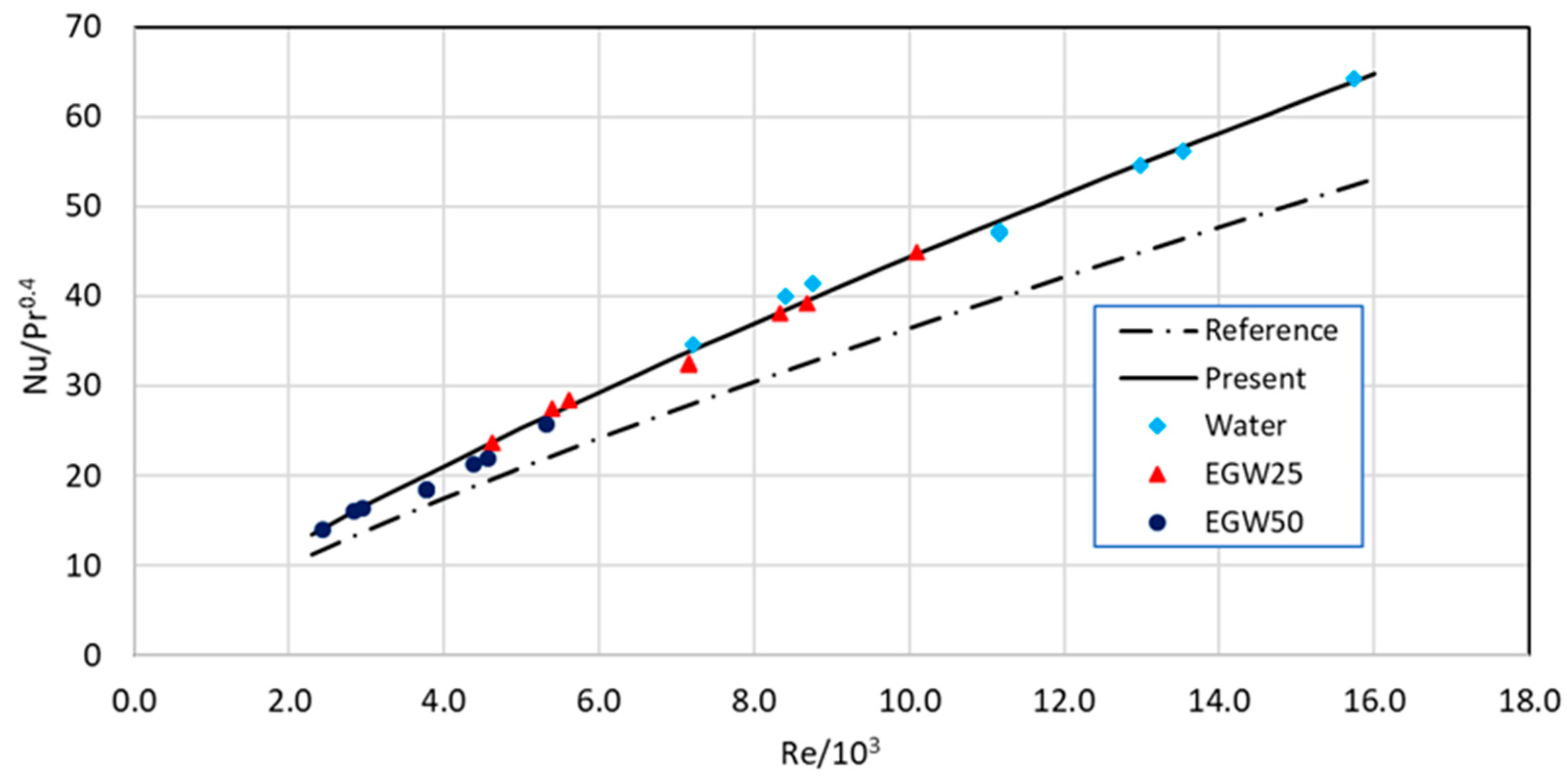
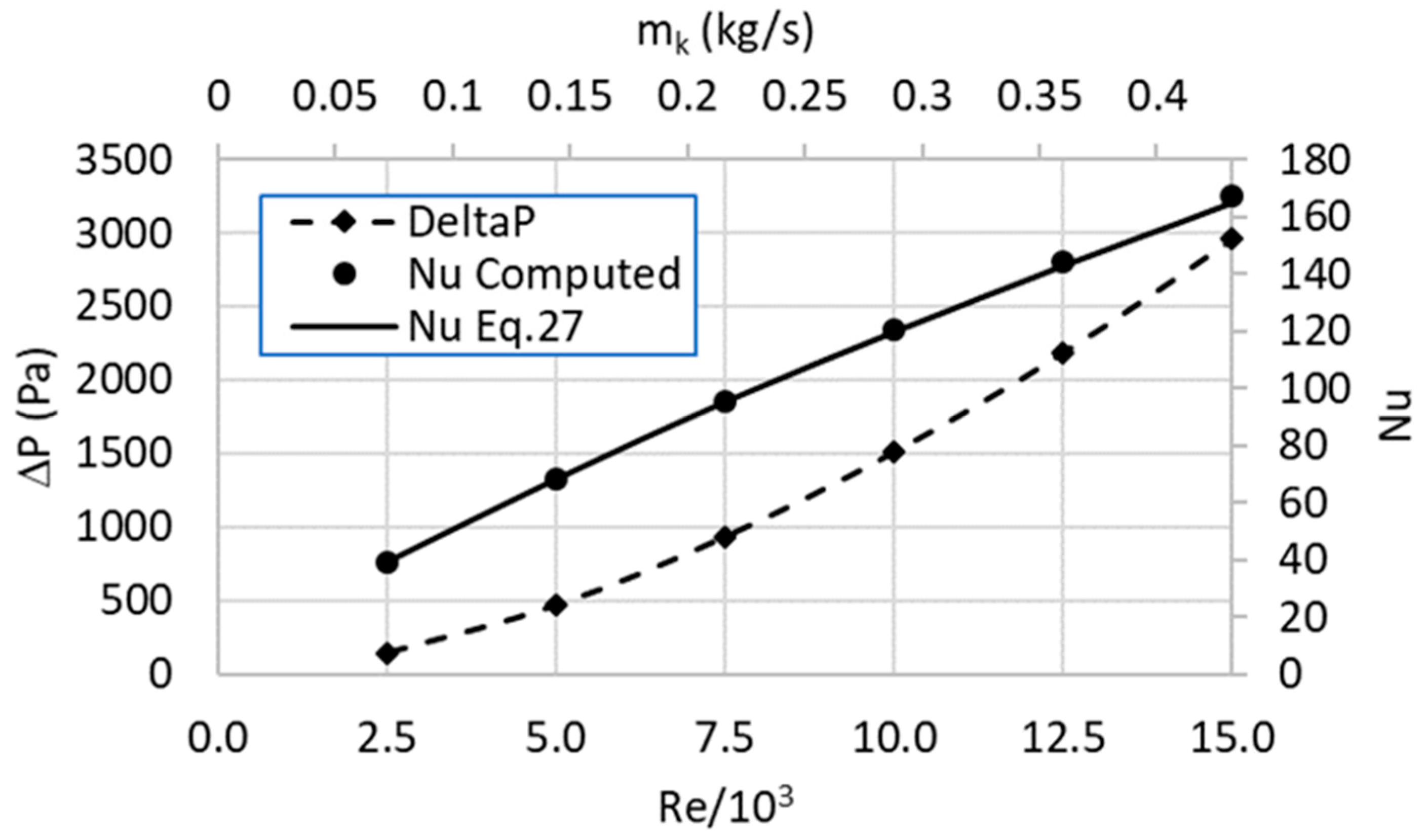
• A new empirical Nusselt number equation is proposed. It predicts Nusselt number within 5% error for all coolant fluids and cases considered in this study. In the sensitivity analysis by using only water and 25% and 50% ethylene glycol–water solutions as the coolant fluid, it shows a perfect agreement with the computed Nusselt number values for Reynolds number ranges from 2500 to 15,000.
• Water as a coolant fluid presents better thermal and hydraulic performance (i.e., smaller T_max, T_mean, T_σ, and ∆P) than the other coolants for the same geometry and working conditions.
• It is also observed that the rise of ethylene glycol ratio in the coolant solution decreases the thermal and the hydraulic performance (i.e., larger T_max, T_mean, T_σ, and ∆P) for the same geometry and working conditions.
• The pressure drop (∆P) is the most influenced parameter from the geometry and mass flow rate. It has significant variation from case to case for all coolant fluids.
• Increasing channel number with a constant total mass flow rate gives a more homogeneous temperature distribution (i.e., smaller T_σ) on the cold plate surface.
• In the Taguchi-based grey relational analysis, the pressure drop with the highest variation with respect to other outcome parameters has the highest weighting factor.
• In the multi-objective optimization, maximizing the number of channels in the cold plate geometry is the common choice for all coolants.
• Weighting factors showing the effect of each result parameter on cooling performance were calculated by Taguchi analysis.
• As a result of the multi-objective optimization, among the three coolant types, water gives the lowest maximum temperature, the best temperature homogeneity, and the lowest pressure drop for the same operating conditions. Meanwhile, EGW 50 coolant gives the worst performance values. It should be mentioned that ethylene glycol–water solutions have lower freezing temperatures, and they can work under sub-zero environmental conditions. It can be also used for the heating to keep the battery temperature in the working temperature range.
• The use of different cold plate designs with hybrid cooling methods for the different battery packs and the comparison of the results with experimental or numerical studies, the use of different fluids, and the effects of transient conditions may be separate research topics in the future.

References

1. Burden, D.; Litman, T. America Needs Complete Streets. ITE J. 2011, 81, 36–43. [Google Scholar]
2. Kennedy, C.A. A Comparison of the Sustainability of Public and Private Transportation Systems: Study of the Greater Toronto Area. Transportation 2002, 29, 459–493. [Google Scholar] [CrossRef]
3. Rojas-Rueda, D.; Nieuwenhuijsen, M.J.; Khreis, H.; Frumkin, H. Autonomous Vehicles and Public Health. Annu. Rev. Public Health 2019, 41, 329–345. [Google Scholar] [CrossRef] [Green Version]
4. Axsen, J.; Plötz, P.; Wolinetz, M. Crafting Strong, Integrated Policy Mixes for Deep CO2 Mitigation in Road Transport. Nat. Clim. Chang. 2020, 10, 809–818. [Google Scholar] [CrossRef]
5. Xia, T.; Zhang, Y.; Crabb, S.; Shah, P. Cobenefits of Replacing Car Trips with Alternative Transportation: A Review of Evidence and Methodological Issues. J. Environ. Public Health 2013, 2013, 797312. [Google Scholar] [CrossRef]
6. Rahman, M.M.; Alam, K.; Velayutham, E. Reduction of CO2 Emissions: The Role of Renewable Energy, Technological Innovation and Export Quality. Energy Rep. 2022, 8, 2793–2805. [Google Scholar] [CrossRef]
7. Horowitz, C.A. Paris Agreement. Int. Leg. Mater. 2016, 55, 740–755. [Google Scholar] [CrossRef]
8. WADA, M. Research and Development of Electric Vehicles for Clean Transportation. J. Environ. Sci. 2009, 21, 745–749. [Google Scholar] [CrossRef]
9. Andersen, P.H.; Mathews, J.A.; Rask, M. Integrating Private Transport into Renewable Energy Policy: The Strategy of Creating Intelligent Recharging Grids for Electric Vehicles. Energy Policy 2009, 37, 2481–2486. [Google Scholar] [CrossRef]
10. Miao, Y.; Hynan, P.; Von Jouanne, A.; Yokochi, A. Current Li-Ion Battery Technologies in Electric Vehicles and Opportunities for Advancements. Energies 2019, 12, 1074. [Google Scholar] [CrossRef] [Green Version]
11. Wang, Q.; Jiang, B.; Li, B.; Yan, Y. A Critical Review of Thermal Management Models and Solutions of Lithium-Ion Batteries for the Development of Pure Electric Vehicles. Renew. Sustain. Energy Rev. 2016, 64, 106–128. [Google Scholar] [CrossRef]
12. Chen, S.C.; Wan, C.C.; Wang, Y.Y. Thermal Analysis of Lithium-Ion Batteries. J. Power Sources 2005, 140, 111–124. [Google Scholar] [CrossRef]
13. Smith, K.; Wang, C.Y. Power and Thermal Characterization of a Lithium-Ion Battery Pack for Hybrid-Electric Vehicles. J. Power Sources 2006, 160, 662–673. [Google Scholar] [CrossRef]
14. Smith, J.; Hinterberger, M.; Schneider, C.; Koehler, J. Energy Savings and Increased Electric Vehicle Range through Improved Battery Thermal Management. Appl. Therm. Eng. 2016, 101, 647–656. [Google Scholar] [CrossRef]
15. Choudhari, V.G.; Dhoble, D.A.S.; Sathe, T.M. A Review on Effect of Heat Generation and Various Thermal Management Systems for Lithium Ion Battery Used for Electric Vehicle. J. Energy Storage 2020, 32, 101729. [Google Scholar] [CrossRef]
16. Zhao, C.; Zhang, B.; Zheng, Y.; Huang, S.; Yan, T.; Liu, X. Hybrid Battery Thermal Management System in Electrical Vehicles: A Review. Energies 2020, 13, 6257. [Google Scholar] [CrossRef]
17. Lv, W.; Li, J.; Chen, M. Experimental Study on the Thermal Management Performance of a Power Battery Module with a Pulsating Heat Pipe under Different Thermal Management Strategies. Appl. Therm. Eng. 2023, 227, 120402. [Google Scholar] [CrossRef]
18. Chen, J.; Kang, S.; Jiaqiang, E.; Huang, Z.; Wei, K.; Zhang, B.; Zhu, H.; Deng, Y.; Zhang, F.; Liao, G. Effects of Different Phase Change Material Thermal Management Strategies on the Cooling Performance of the Power Lithium Ion Batteries: A Review. J. Power Sources 2019, 442, 227228. [Google Scholar] [CrossRef]
19. Souayfane, F.; Fardoun, F.; Biwole, P.H. Phase Change Materials (PCM) for Cooling Applications in Buildings: A Review. Energy Build. 2016, 129, 396–431. [Google Scholar] [CrossRef]
20. Aslan, E.; Aydın, Y.; Yaşa, Y. Consideration of Graphene Material in PCM with Aluminum Fin Structure for Improving the Battery Cooling Performance. Int. J. Energy Res. 2022, 46, 10758–10769. [Google Scholar] [CrossRef]
21. Joula, M.; Dilibal, S.; Mafratoglu, G.; Danquah, J.O.; Alipour, M. Hybrid Battery Thermal Management System with NiTi SMA and Phase Change Material (PCM) for Li-Ion Batteries. Energies 2022, 15, 4403. [Google Scholar] [CrossRef]
22. Abdulrasool Hasan, H.; Togun, H.; Abed, A.M.; I Mohammed, H.; Biswas, N. A Novel Air-Cooled Li-Ion Battery (LIB) Array Thermal Management System—A Numerical Analysis. Int. J. Therm. Sci. 2023, 190, 108327. [Google Scholar] [CrossRef]
23. Hasan, H.A.; Togun, H.; Abed, A.M.; Biswas, N.; Mohammed, H.I. Thermal Performance Assessment for an Array of Cylindrical Lithium-Ion Battery Cells Using an Air-Cooling System. Appl. Energy 2023, 346, 121354. [Google Scholar] [CrossRef]
24. Gungor, S. Analytical and Numerical Investigations on Optimal Cell Spacing for Air-Cooled Energy Storage Systems. Int. J. Therm. Sci. 2023, 191, 108332. [Google Scholar] [CrossRef]
25. Panchal, S.; Dincer, I.; Agelin-Chaab, M.; Fraser, R.; Fowler, M. Thermal Modeling and Validation of Temperature Distributions in a Prismatic Lithium-Ion Battery at Different Discharge Rates and Varying Boundary Conditions. Appl. Therm. Eng. 2016, 96, 190–199. [Google Scholar] [CrossRef]
26. Sundén, B. Thermal Management of Batteries. In Hydrogen, Batteries and Fuel Cells; Academic Press: Cambridge, MA, USA, 2019; pp. 93–110. ISBN 978-0-12-816950-6. [Google Scholar]
27. Kim, J.; Oh, J.; Lee, H. Review on Battery Thermal Management System for Electric Vehicles. Appl. Therm. Eng. 2019, 149, 192–212. [Google Scholar] [CrossRef]
28. Kummitha, O.R. Thermal Cooling of Li-Ion Cylindrical Cells Battery Module with Baffles Arrangement for Airflow Cooling Numerical Analysis. J. Energy Storage 2023, 59, 106474. [Google Scholar] [CrossRef]
29. Jiaqiang, E.; Xu, S.; Deng, Y.; Zhu, H.; Zuo, W.; Wang, H.; Chen, J.; Peng, Q.; Zhang, Z. Investigation on Thermal Performance and Pressure Loss of the Fluid Cold-Plate Used in Thermal Management System of the Battery Pack. Appl. Therm. Eng. 2018, 145, 552–568. [Google Scholar] [CrossRef]
30. Deng, Y.; Feng, C.; Jiaqiang, E.; Zhu, H.; Chen, J.; Wen, M.; Yin, H. Effects of Different Coolants and Cooling Strategies on the Cooling Performance of the Power Lithium Ion Battery System: A Review. Appl. Therm. Eng. 2018, 142, 10–29. [Google Scholar] [CrossRef]
31. Chen, D.; Jiang, J.; Kim, G.H.; Yang, C.; Pesaran, A. Comparison of Different Cooling Methods for Lithium Ion Battery Cells. Appl. Therm. Eng. 2016, 94, 846–854. [Google Scholar] [CrossRef] [Green Version]
32. Huo, Y.; Rao, Z.; Liu, X.; Zhao, J. Investigation of Power Battery Thermal Management by Using Mini-Channel Cold Plate. Energy Convers. Manag. 2015, 89, 387–395. [Google Scholar] [CrossRef]
33. Li, M.; Wang, J.; Guo, Q.; Li, Y.; Xue, Q.; Qin, G. Numerical Analysis of Cooling Plates with Different Structures for Electric Vehicle Battery Thermal Management Systems. J. Energy Eng. 2020, 146, 04020037. [Google Scholar] [CrossRef]
34. Benabdelaziz, K.; Lebrouhi, B.; Maftah, A.; Maaroufi, M. Novel External Cooling Solution for Electric Vehicle Battery Pack. Energy Reports 2020, 6, 262–272. [Google Scholar] [CrossRef]
35. Mei, N.; Xu, X.; Li, R. Heat Dissipation Analysis on the Liquid Cooling System Coupled with a Flat Heat Pipe of a Lithium-Ion Battery. ACS Omega 2020, 5, 17431–17441. [Google Scholar] [CrossRef]
36. Lan, C.; Xu, J.; Qiao, Y.; Ma, Y. Thermal Management for High Power Lithium-Ion Battery by Minichannel Aluminum Tubes. Appl. Therm. Eng. 2016, 101, 284–292. [Google Scholar] [CrossRef] [Green Version]
37. Zhao, J.; Rao, Z.; Li, Y. Thermal Performance of Mini-Channel Liquid Cooled Cylinder Based Battery Thermal Management for Cylindrical Lithium-Ion Power Battery. Energy Convers. Manag. 2015, 103, 157–165. [Google Scholar] [CrossRef]
38. Bulut, E.; Albak, E.İ.; Sevilgen, G.; Öztürk, F. A New Approach for Battery Thermal Management System Design Based on Grey Relational Analysis and Latin Hypercube Sampling. Case Stud. Therm. Eng. 2021, 28, 101452. [Google Scholar] [CrossRef]
39. Kumar, K.; Pareek, K. Fast Charging of Lithium-Ion Battery Using Multistage Charging and Optimization with Grey Relational Analysis. J. Energy Storage 2023, 68, 107704. [Google Scholar] [CrossRef]
40. Jiang, L.; Li, Y.; Huang, Y.; Yu, J.; Qiao, X.; Wang, Y.; Huang, C.; Cao, Y. Optimization of Multi-Stage Constant Current Charging Pattern Based on Taguchi Method for Li-Ion Battery. Appl. Energy 2020, 259, 114148. [Google Scholar] [CrossRef]
41. Mo, X.; Zhi, H.; Xiao, Y.; Hua, H.; He, L. Topology Optimization of Cooling Plates for Battery Thermal Management. Int. J. Heat Mass Transf. 2021, 178, 121612. [Google Scholar] [CrossRef]
42. Ye, B.; Rubel, M.R.H.; Li, H. Design and Optimization of Cooling Plate for Battery Module of an Electric Vehicle. Appl. Sci. 2019, 9, 754. [Google Scholar] [CrossRef] [Green Version]
43. Egab, K.; Oudah, S.K. Thermal Management Analysis of Li-Ion Battery-Based on Cooling System Using Dimples with Air Fins and Perforated Fins. Int. J. Therm. Sci. 2022, 171, 107200. [Google Scholar] [CrossRef]
44. Ling, Z.; Cao, J.; Zhang, W.; Zhang, Z.; Fang, X.; Gao, X. Compact Liquid Cooling Strategy with Phase Change Materials for Li-Ion Batteries Optimized Using Response Surface Methodology. Appl. Energy 2018, 228, 777–788. [Google Scholar] [CrossRef]
45. Naqiuddin, N.H.; Saw, L.H.; Yew, M.C.; Yusof, F.; Poon, H.M.; Cai, Z.; Thiam, H.S. Numerical Investigation for Optimizing Segmented Micro-Channel Heat Sink by Taguchi-Grey Method. Appl. Energy 2018, 222, 437–450. [Google Scholar] [CrossRef] [Green Version]
46. Jiaqiang, E.; Han, D.; Qiu, A.; Zhu, H.; Deng, Y.; Chen, J.; Zhao, X.; Zuo, W.; Wang, H.; Chen, J.; et al. Orthogonal Experimental Design of Liquid-Cooling Structure on the Cooling Effect of a Liquid-Cooled Battery Thermal Management System. Appl. Therm. Eng. 2018, 132, 508–520. [Google Scholar] [CrossRef]
47. Kılıç, M.; Şentürk, S. Application of Multi-Response Taguchi Method on the Optimization of a Mini-Channel Cooling Block for the Developing Laminar Flow. Uludağ Univ. J. Fac. Eng. 2019, 24, 433–450. [Google Scholar] [CrossRef]
48. Sato, N. Thermal Behavior Analysis of Lithium-Ion Batteries for Electric and Hybrid Vehicles. J. Power Sources 2001, 99, 70–77. [Google Scholar] [CrossRef]
49. Siemens Digital Industries Software AMESIM; Siemens: Madison, WI, USA, 2021.
50. Bernardi, D.; Pawlikowski, E.; Newman, J. General Energy Balance for Battery Systems. Electrochem. Soc. Ext. Abstr. 1984, 84–82, 164–165. [Google Scholar] [CrossRef] [Green Version]
51. Ding, Y.; Wei, M.; Liu, R. Parameters of liquid cooling thermal management system effect on the li-ion battery temperature distribution. Therm. Sci. 2022, 26, 567–577. [Google Scholar] [CrossRef]
52. Kılıç, M.; Yiğit, A. Heat Transfer, 6th ed.; Dora Publishing: Bursa, Turkey, 2018; ISBN 978-605-247-037-4. (In Turkish) [Google Scholar]
53. Klein, S.A. Engineering Equation Solver (EES); F-Chart Software: Madison, WI, USA, 2015. [Google Scholar]
54. Sevilgen, G.; Kiliç, M.; Aktas, M. Dual-Separated Cooling Channel Performance Evaluation for High-Power Led Pcb in Automotive Headlight. Case Stud. Therm. Eng. 2021, 25, 100985. [Google Scholar] [CrossRef]
55. Patankar, S. Numerical Heat Transfer and Fluid Flow; CRC Press: Boca Raton, FL, USA, 2018; ISBN 9781315275130. [Google Scholar]
56. ANSYS. Ansys Fluent 19.0 Theory Guide; Release 19; ANSYS Inc.: Canonsburg, PA, USA, 2021. [Google Scholar]
57. Wilcox, D.C. Formulation of the K-w Turbulence Model Revisited. AIAA J. 2008, 46, 2823–2838. [Google Scholar] [CrossRef] [Green Version]
58. Jarrett, A.; Kim, I.Y. Design Optimization of Electric Vehicle Battery Cooling Plates for Thermal Performance. J. Power Sources 2011, 196, 10359–10368. [Google Scholar] [CrossRef]
59. Kilic, M.; Aktas, M.; Sevilgen, G. Thermal Assessment of Laminar Flow Liquid Cooling Blocks for LED Circuit Boards Used in Automotive Headlight Assemblies. Energies 2020, 13, 1202. [Google Scholar] [CrossRef] [Green Version]
60. Tzeng, C.J.; Lin, Y.H.; Yang, Y.K.; Jeng, M.C. Optimization of Turning Operations with Multiple Performance Characteristics Using the Taguchi Method and Grey Relational Analysis. J. Mater. Process. Technol. 2009, 209, 2753–2759. [Google Scholar] [CrossRef]
61. Sahin, B. A Taguchi Approach for Determination of Optimum Design Parameters for a Heat Exchanger Having Circular-Cross Sectional Pin Fins. Heat Mass Transf. Stoffuebertragung 2007, 43, 493–502. [Google Scholar] [CrossRef]
62. Wang, X. Application of Grey Relation Analysis Theory to Choose High Reliability of the Network Node. J. Phys. Conf. Ser. 2019, 1237, 032056. [Google Scholar] [CrossRef] [Green Version]
63. Özdemir Küçük, E.; Kılıç, M. Exergoeconomic Analysis and Multi-Objective Optimization of ORC Configurations via Taguchi-Grey Relational Methods. Heliyon 2023, 9, 1–25. [Google Scholar] [CrossRef]
64. Chamoli, S.; Yu, P.; Kumar, A. Multi-Response Optimization of Geometric and Flow Parameters in a Heat Exchanger Tube with Perforated Disk Inserts by Taguchi Grey Relational Analysis. Appl. Therm. Eng. 2016, 103, 1339–1350. [Google Scholar] [CrossRef]
65. Asafa, T.B.; Bryce, G.; Severi, S.; Said, S.A.M.; Witvrouw, A. Multi-Response Optimization of Ultrathin Poly-SiGe Films Characteristics for Nano-ElectroMechanical Systems (NEMS) Using the Grey-Taguchi Technique. Microelectron. Eng. 2013, 111, 229–233. [Google Scholar] [CrossRef]
66. Bademlioglu, A.H.; Canbolat, A.S.; Kaynakli, O. Multi-Objective Optimization of Parameters Affecting Organic Rankine Cycle Performance Characteristics with Taguchi-Grey Relational Analysis. Renew. Sustain. Energy Rev. 2020, 117, 109483. [Google Scholar] [CrossRef]
67. Dittus, F.W.; Boelter, L.M.K. Heat Transfer in Automobile Radiators of the Tubular Type. In University of California Publications in Engineering; University of California Press: Berkeley, CA, USA, 1930; pp. 443–461. [Google Scholar]
Figure 1. A 1D generic battery model.
Sustainability 15 12391 g001
Figure 2. Battery pre-sizing tool: (A) Main input parameters; (B) Calculated results; (C) Variation of variables based on different temperatures.
Sustainability 15 12391 g002
Figure 3. Comparison of the potential values obtained from the AMESIM model and the test bench.
Sustainability 15 12391 g003
Figure 4. Heat flux analysis: (a) obtained heat flux value, (b) SOC percentage.
Sustainability 15 12391 g004
Figure 5. Geometry structure: (a) Placement of the cold plate between the battery packs; (b) Channel cross-section geometry details.
Sustainability 15 12391 g005
Figure 6. The 3D geometry of cold plate geometries: (a) 4-channel; (b) 5-channel; (c) 6-channel.
Sustainability 15 12391 g006
Figure 7. Mesh structure was employed in CFD analysis: (A) Cold plate mesh structure; (B) Mesh details in channel bends; (C) Mesh details in channel walls.
Sustainability 15 12391 g007
Figure 8. Comparison of Tmax and ΔP values obtained from different meshes. Mesh independency analysis in CFD analysis.
Sustainability 15 12391 g008
Figure 9. Variation of Nusselt number with Reynolds number for all the cases.
Sustainability 15 12391 g009
Figure 10. Temperature distributions on the bottom surface of the cold plate for the optimized cases: (a) L8 for fluid water; (b) L8 for fluid EGW 25; (c) L9 for fluid EGW 50.
Sustainability 15 12391 g010
Figure 11. The effect of Reynolds number on the Tmax, Tmean, and Tσ of the optimized cold plate surface by using water as coolant.
Sustainability 15 12391 g011
Figure 12. The effect of Reynolds number on the ΔP and Nusselt number for the optimized cold plate by using water as coolant.
Sustainability 15 12391 g012
Figure 13. The effect of Reynolds number on the Tmax, Tmean, and Tσ of the optimized cold plate surface by using EGW 25 as coolant.
Sustainability 15 12391 g013
Figure 14. The effect of Reynolds number on the ΔP and Nusselt number for the optimized cold plate by using EGW 25 as coolant.
Sustainability 15 12391 g014
Figure 15. The effect of Reynolds number on the Tmax, Tmean, and Tσ of the optimized cold plate surface by using EGW 50 as coolant.
Sustainability 15 12391 g015
Figure 16. The effect of Reynolds number on the ΔP and Nusselt number for the optimized cold plate by using EGW 50 as coolant.
Sustainability 15 12391 g016
Figure 17. The effect of Reynolds number on the required pump power, W ˙ , for the optimized cold plate by using water, EGW 25, and EGW 50 as coolant.
Sustainability 15 12391 g017