Evaluation the Resistance Growth of Aged Vehicular Proton Exchange Membrane Fuel Cell Stack by Distribution of Relaxation Times

Abstract

The aged stack results in resistance growth and power decline. At present, most of the analyses of resistance growth are qualitative or identified by complex mechanism models. For more effective identification, the distribution of relaxation times (DRT) method is applied to the aging analysis of the stack. The individual polarization process of the stack corresponding to each DRT peak is determined by appropriate experimental conditions and the impedance of the individual polarization process is characterized by the peak area. The three DRT peaks from low frequency to high frequency are identified as the mass transport, the charge transfer of oxygen reduction reactions (ORRs), and the proton transport in the cathode catalyst layer (CCL) and anode side. The stack’s voltage recession rate is 15% at the rated current density of 800 mA cm⁻² after running for 2000 h in the driving cycle. Mass transport is the main reason accounting for 66.1% of the resistance growth. The charge transfer resistance growth cannot be ignored, accounting for 30.23%. The resistance growth obtained by the DRT can quickly and accurately identify the main reason for stack decline and therefore promises to become an important diagnostic tool in relation to aging.

1. Introduction

Aging is one of the key issues restricting the commercialization of proton exchange membrane fuel cells (PEMFCs) [1,2]. Long time operations of starting/stopping [3], load changing [4], and poor water and heat management [5,6] can lead to performance degradation, manifesting in the increased polarization loss of PEMFCs.

The methods used to explain polarization loss can be mainly divided into two categories: postmortem [1,7,8,9,10] and in situ [11,12,13,14,15,16,17] diagnostic techniques. For the postmortem method, it is usually required to decompose the aged stacks, and the morphology analysis of the membrane electrode assembly (MEA) and gas diffusion layer (GDL)/microporous layer (MPL) is carried out. The problem with this method is that the microstructure of the MEA and GDL/MPL will be destroyed in the process of decomposition. By contrast, in situ methods do not have such problems.

Among the in situ methods, electrochemical impedance spectroscopy (EIS) has a powerful electrochemical analysis capability that can distinguish polarization processes of mass transport, charge transfer, and proton transport in different frequency domains [18,19,20,21,22,23]. The principle of EIS is based on applying harmonic disturbances to an electrochemical system and measuring the impedance of the system over a wide frequency range. EIS is sensitive to both the internal material parameters and external operating conditions of electrochemical systems. Owing to the above characteristics and advantages, EIS has great potential in the fields of material development, structural design parameter optimization, and fault diagnosis [20]. In addition, EIS can be used to identify electrode degradation as a valid symbol for evaluating the health of PEMFCs exposed to accelerated stress tests [19]. However, interpreting measured EIS data in an appropriate way can be challenging. Equivalent circuit models (ECMs) composed of equivalent electrical elements can be used to interpret EIS data [24,25]. The equivalent circuit elements include resistance, inductance, capacitance, constant phase element (CPE), Warburg element, etc. [20]. At present, there are at least six basic ECMs for PEMFCs [20], and many variations on this basis. Each ECM has its own application scenarios. Therefore, the proper use of an ECM requires prior knowledge of the fuel cell system in order to use the model to describe the electrochemical process accurately and the interpretation is always ambiguous because different models might fit the same EIS measurement data [26,27,28].

To avoid these problems linked with ECMs, the distribution of relaxation times (DRT), a complementary method that can enhance the analytical ability of ECMs, has been developed. DRT can identify the time constant of the electrochemical process without considering the exact internal mechanism by the quasi-infinite series of R//C elements, so there is no need for prior knowledge. The DRT method has been applied to the aging analysis of solid oxide fuel cells [29,30,31] and lithium-ion batteries [32,33] because of its excellent resolution capability of the individual polarization process. In the field of PEMFCs, DRT is mainly used to analyze the relationship between polarization loss at different time constants and electrochemical reaction processes [34,35,36]. Weiß et al. [36] first applied the DRT method to impedance analysis of PEMFCs, and seven peaks were identified in the DRT function. The peaks in the DRT function were interpreted with the cell’s internal phenomena by a set of experimental conditions (current density, air stoichiometry, etc.). Heinzmann et al. [35] identified a PEMFC’s polarization processes by setting a wide range of operating conditions, including current densities, relative humidity, and various cathode and anode gas compositions. The results showed that the peaks of DRT function from low frequency to high frequency are related to the mass transport process, the charge transfer process, and proton transfer in the cathode catalyst layer (CCL), respectively. Kulikovsky et al. [34] proposed a simple numerical method for the calculation of DRT for PEMFC impedance. The relationship between the oxygen transfer peak of DRT and the oxygen transfer coefficient in CCL was studied by this method and it was used as an indicator for cathode flooding. Yuan et al. [23] established a two-dimensional impedance model of a PEMFC to qualitatively analyze the electrochemical polarization process represented by DRT distribution. A systematic dynamic configuration and model analysis results have shown that the polarization processes form ultra-high frequency to ultra-low frequency correspond to anode charge transfer, proton transfer in the CCL, charge transfer in the cathode, oxygen transport in the cathode, and dissolved water transport, respectively.

Although the above studies have played a great role in promoting the application of DRT in PEMFC design, some aspects are not covered. Firstly, most of the above studies on PEMFCs are qualitative analyses of the polarization process represented by DRT distribution which involved changing experimental conditions or impedance models but lack quantitative analysis of the resistance of each polarization process through DRT distribution, namely, DRT peaks. In addition, there are few studies on the aging analysis of PEMFCs using the DRT method, although DRT has been applied in the aging analysis of lithium-ion batteries [33] and solid oxide fuel cells [31]. This paper aims to explore the application of the DRT method in aging analysis of PEMFCs.

In this paper, the DRT method is used to quantitatively analyze the resistance growth of the aged vehicular PEMFC stack. The main idea and the analysis procedure are shown in Figure 1. Firstly, the internal polarization process corresponding to each DRT peak is analyzed and verified by appropriate experiments. Secondly, the polarization resistance is calculated by the area of the DRT peak and resistance growth analyses of the aged vehicular PEMFC stack using the DRT, ECM, and I–V polarization curves are compared. Finally, it is concluded that the DRT method is effective in analyzing the aged stack and the main reason for the resistance growth is mass transport.

2. Materials and Methods

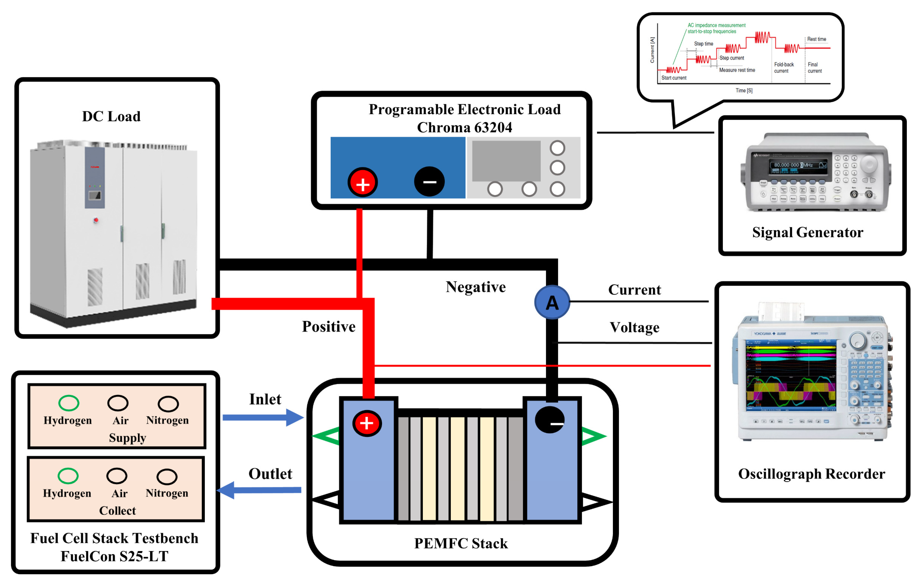
2.1. The PEMFC Stack and Test Bench

The large-scale PEMFC stack manufactured by PowerCell Sweden AB in Gothenburg, Sweden is used for the experiments.

Table 1. Key parameters of the stack.

Parameters	Values
Specification	S2
Pitch number	216
Electrochemical active area	195 cm2
Cathode/anode Pt loading	0.4 mg cm−2/0.1 mg cm−2
Rated output power of stack	22.6 kW
Rated current of stack (0.67 V)	156 A
Maximum output power of stack	30.3 kW
Maximum current of stack (0.6 V)	234 A
Working temperature	70~80 °C
Bipolar plate	Metal
Flow field	Counter flow

shows the key parameters of the stack. In order to ensure the output efficiency of the system, we define the single cell voltage of 0.67 V as the rated point of the stack.

The PEMFC stack test bench of FuelCon S25-LT (HORIBA FuelCon GmbH/Germany) is used for gas supply and current loading for the stack, controlling the inlet temperature, humidity, pressure, flow rate of gases, cooling water temperature, and the current of the direct current (DC) load. Self-made AC impedance equipment is used for the superposition of excitation current and the acquisition and processing of signals; an illustration is shown in Figure 2. The EIS of the PEMFC stack is measured under different current densities through a programable electronic load (Chroma 63204 (Chroma ATE Inc./Taiwan, China)) by sweeping frequencies generated by a signal generator covering the range of 2 kHz to 0.4 Hz, with three points per decade. The AC amplitude is set as 5% of the DC load as the galvanostatic mode to perform a linear response. The oscillograph recorder collects the total voltage and total current of the PEMFC stack for impedance calculation.

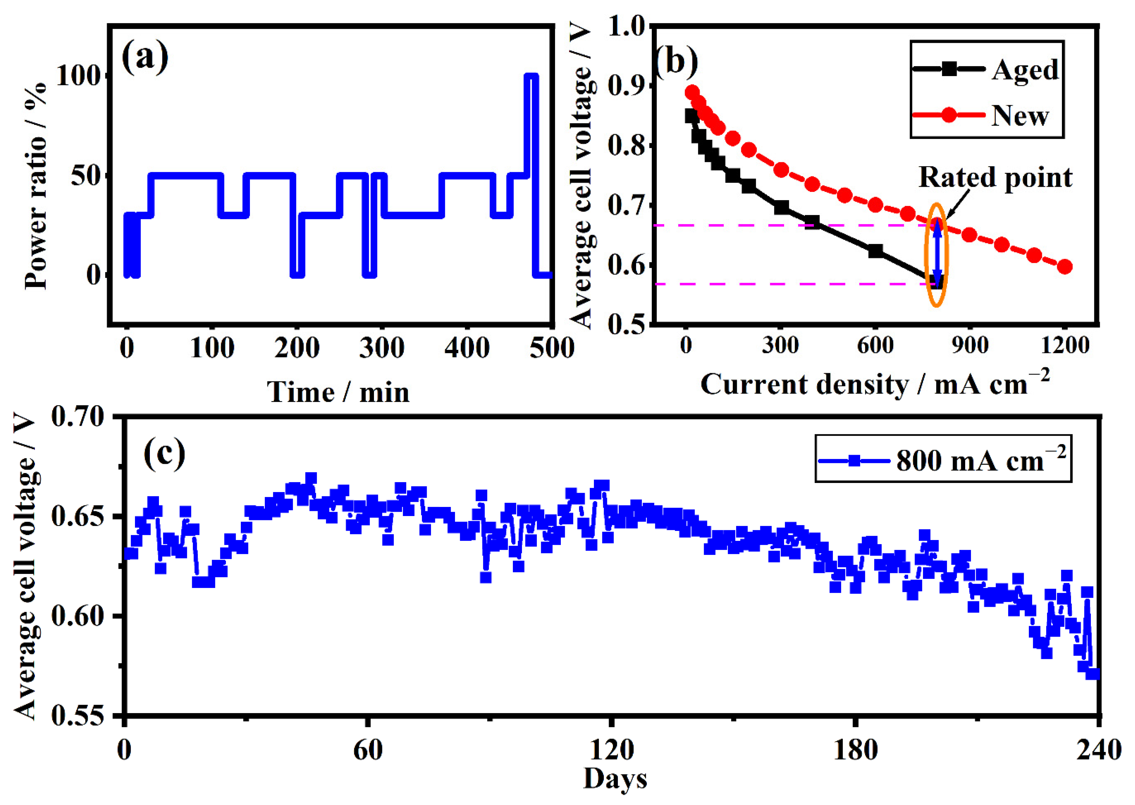
2.2. Procedure of the Experimental Test

Before the EIS test, the experimental stack is operated steadily under the operating conditions in

Table 2. The operation conditions of the PEMFC stack.

Parameters	Values
Operating temperature	70 °C
Anode relative humidity	60%
Current density	20~800 mA cm−2
Cathode relative humidity	80%
Anode stoichiometry	1.5
Cathode stoichiometry	2
Anode pressure	0.85 bar
Cathode pressure	0.75 bar

for 1 h at 500 mA cm⁻² to ensure the repeatability of the results. The operating variable of current densities for the EIS and polarization curve test of the new stack covers 20 mA cm⁻² to 1200 mA cm⁻² and the other operation conditions are referred to in Table 2. For the aged stack, the current densities range covers 20 mA cm⁻² to 800 mA cm⁻². It operates for 15 min to ensure the validity of the test after changing the current density, and each point of current density is measured three times.

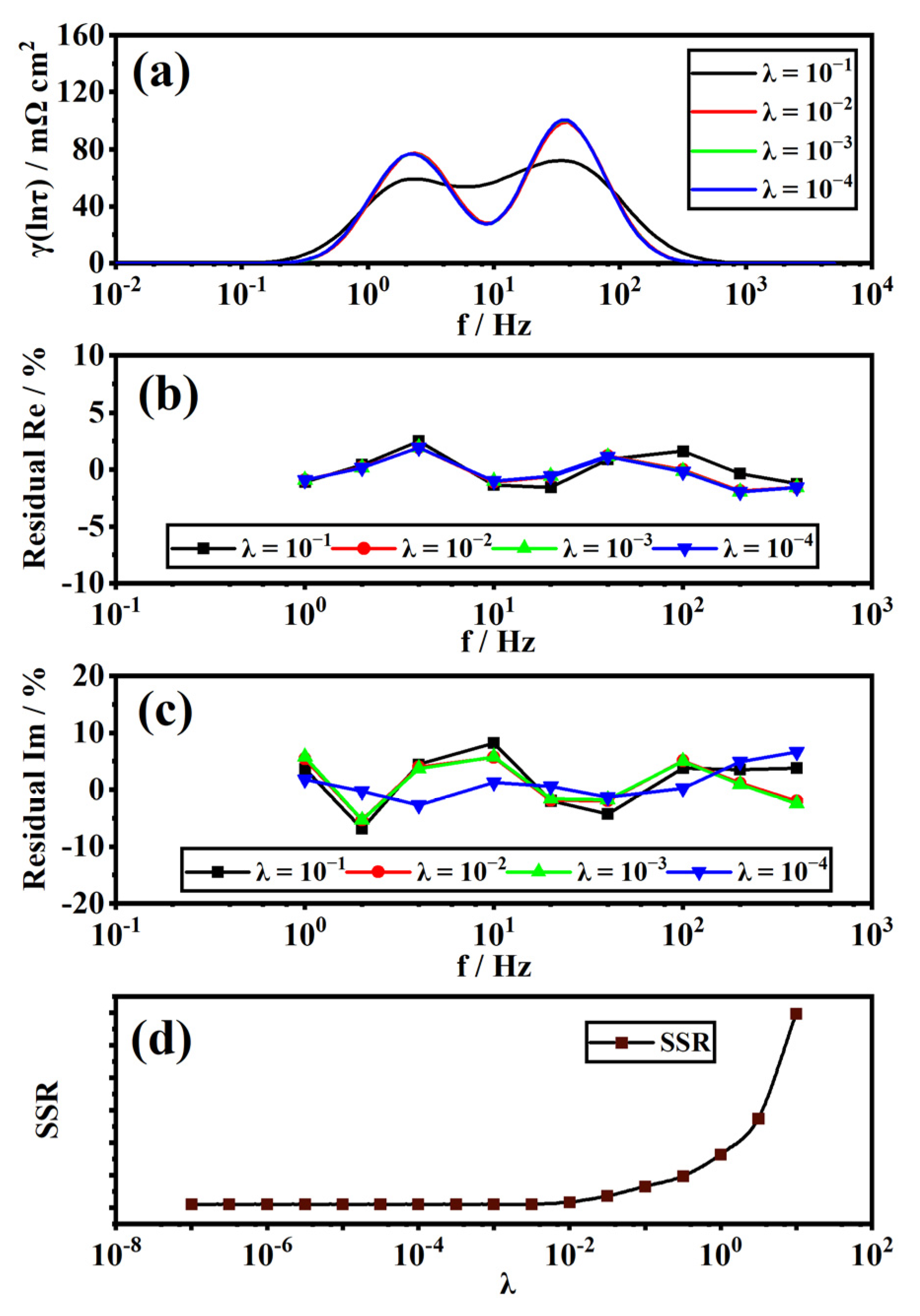
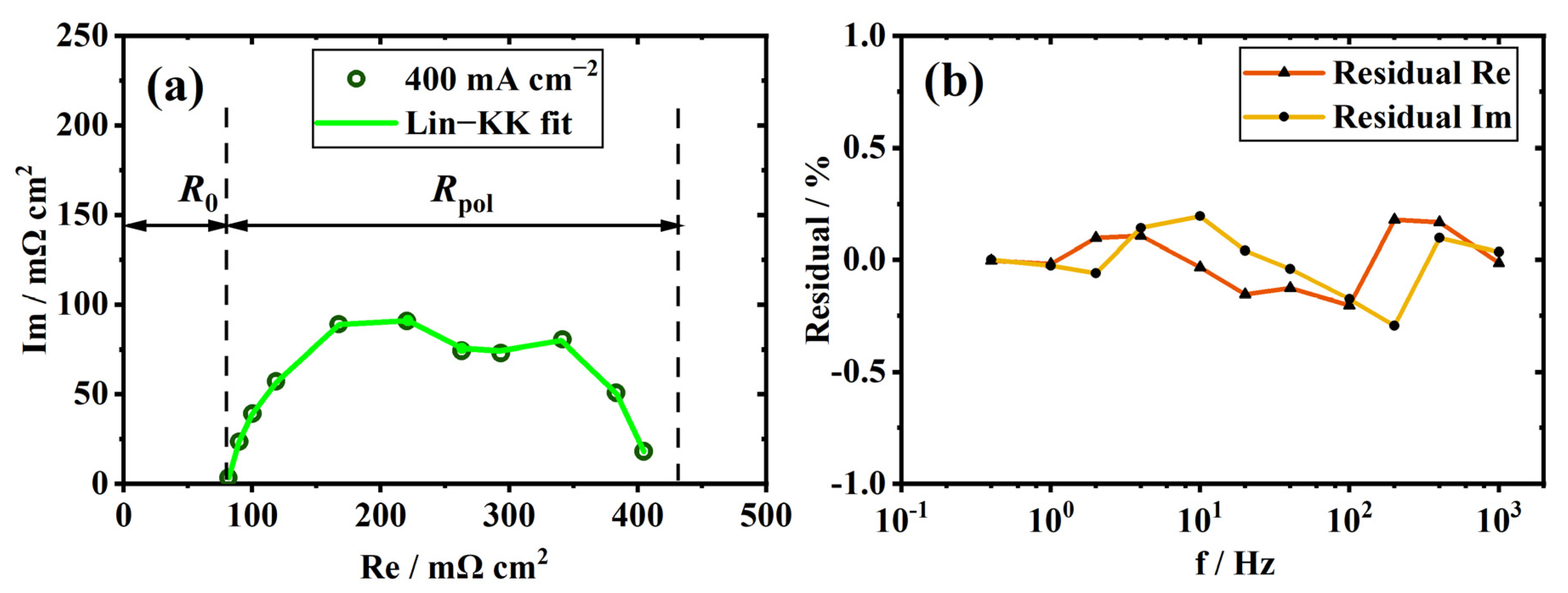
2.3. Kramers–Kronig Validity Test

The quality of the measured impedance data needs to be evaluated in order to effectively analyze the data and interpret the physical significance. The validity of measured impedance spectra is necessary before further analysis, which needs to meet the requirements of linearity, time-invariance, and causality. At present, the verification method of the Kramers–Kronig (KK) transformation is widely used [37]. For a linear, time-invariant, and causal system, the real part $Z_{\mathrm{Re}}(\omega )$ and imaginary part $Z_{\mathrm{Im}}(\omega )$ of the impedance spectrum are related. The equations are as follows:

$$Z_{\mathrm{Re}}(\omega )=\frac{2}{\pi }{\int }_0^{\infty }\frac{{\omega }^{\prime }·Z_{\mathrm{Im}}\left({\omega }^{\prime }\right)}{({{\omega }^{\prime }}^2-{\omega }^2)}d{\omega }^{\prime }$$

(1)

$$Z_{\mathrm{Im}}(\omega )=-\frac{2}{\pi }{\int }_0^{\infty }\frac{\omega ·Z_{\mathrm{Re}}\left({\omega }^{\prime }\right)}{({{\omega }^{\prime }}^2-{\omega }^2)}d{\omega }^{\prime }$$

(2)

where $\omega$ represents the radian frequency. However, the semi-infinite integral can hardly be resolved. To overcome this problem, an approach without direct calculation of the Equations (1) and (2) is proposed, in which the consistency of the impedance spectrum and KK transformation is judged by an appropriate equivalent circuit model (ECM) conforming to KK relations [24,38]. To overcome the nonlinearity of the fitting, there is a method that uses an equivalent circuit model consisting of a resistor in series with a number of R//C elements and fits to the measured impedance data in the form of ohmic resistance and a time constant [39,40]. The validity of the data can be verified quickly by this method. In order to judge the repeatability of the measured impedance data and the KK fitted ECM, the deviation is represented in residuals. The equations are as follows:

$${\Delta }_{\mathrm{Re}}(\omega )=\frac{Z_{\mathrm{Re}}(\omega )-{\widehat{Z}}_{\mathrm{Re}}(\omega )}{\left|Z(\omega )\right|}$$

(3)

$${\Delta }_{\mathrm{Im}}(\omega )=\frac{Z_{\mathrm{Im}}(\omega )-{\widehat{Z}}_{\mathrm{Im}}(\omega )}{\left|Z(\omega )\right|}$$

(4)

where ${\widehat{Z}}_{\mathrm{Re}}(\omega )$ represents the real part of the model impedance, ${\widehat{Z}}_{\mathrm{Im}}(\omega )$ represents the imaginary part of the model impedance, and $\left|Z(\omega )\right|$ represents the absolute value of the measured impedance spectrum. In this paper, Lin−KK Tools software (https://www.iam.kit.edu/wet/english/Lin-KK.php (accessed on 7 April 2022)) [40] is used to produce the fitted ECM and calculate the residual between the data and the model. The impedance data is considered to conform to the KK relations when the relative residual is less than 1%.

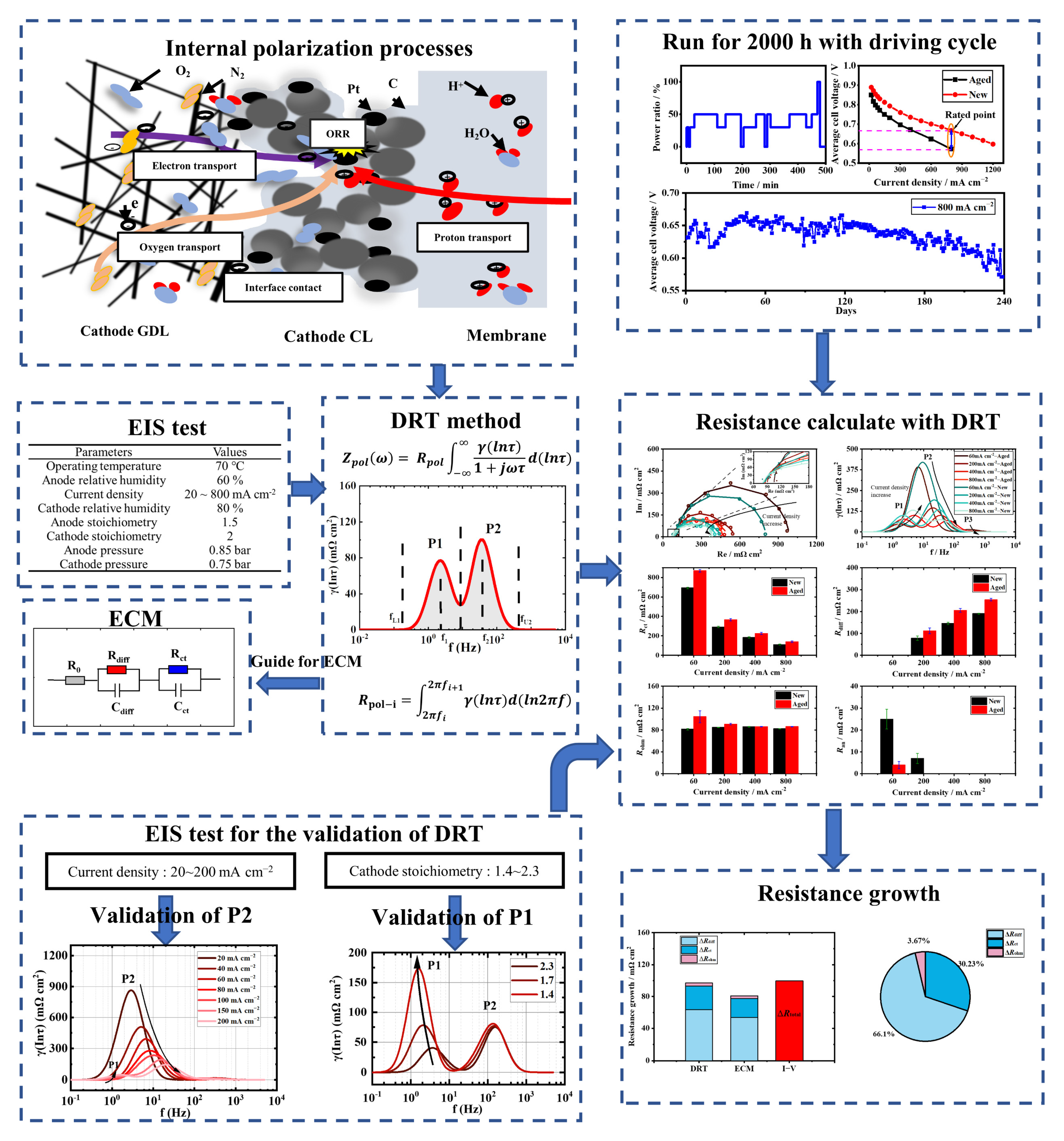
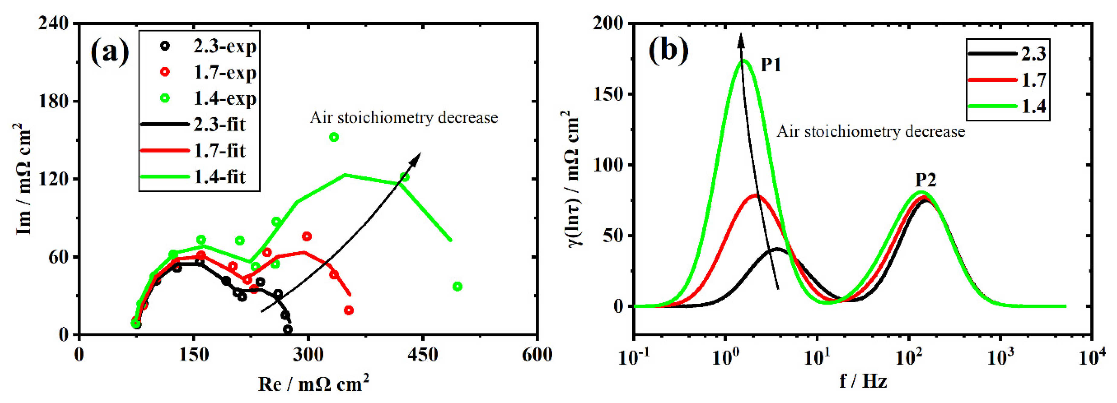
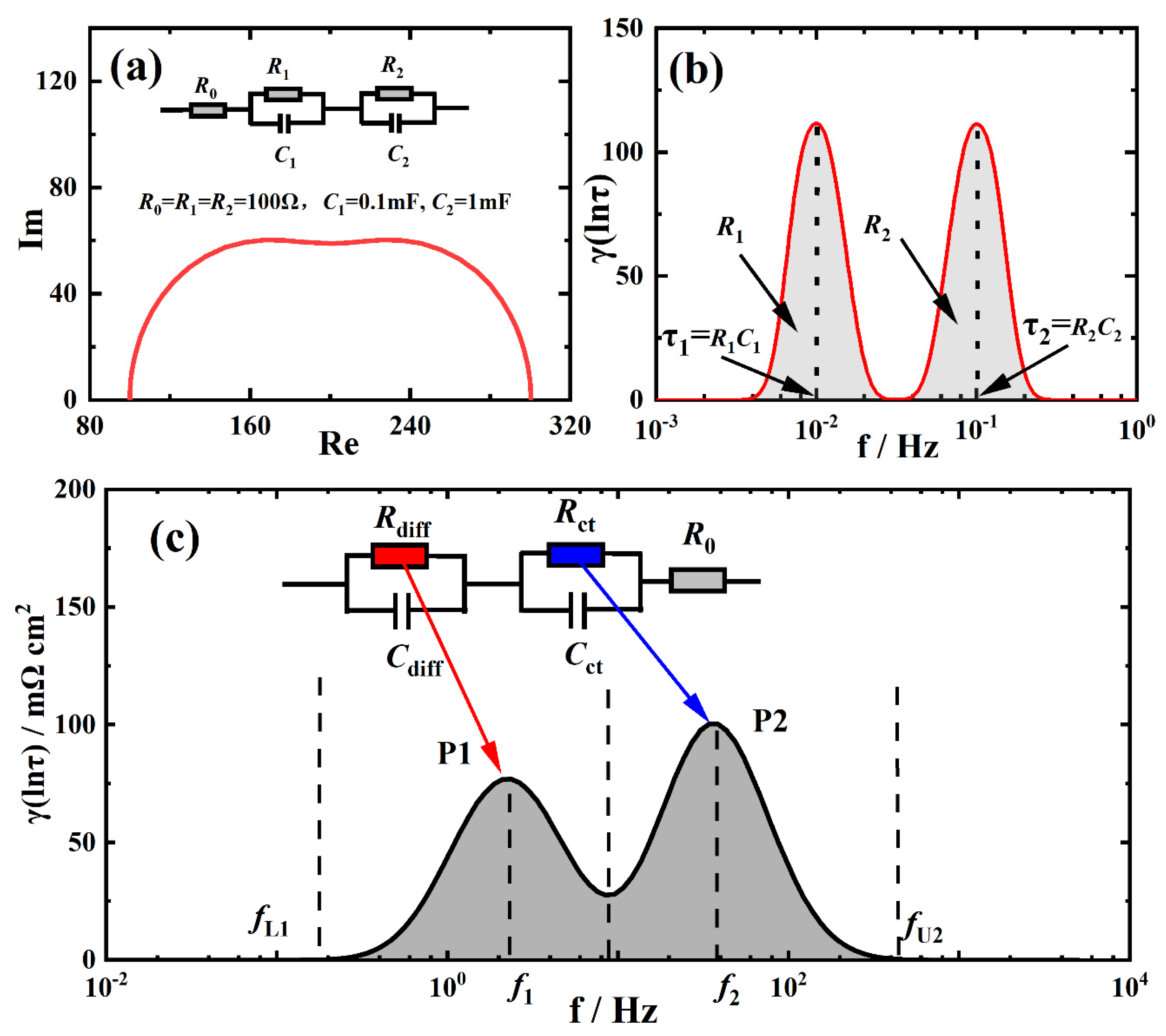
2.4. Distribution of Relaxation Times

DRT identifies each electrochemical process through an intrinsic relaxation time constant, and the amplitude of each time constant represents the strength of the impedance of each electrochemical process. The relationship between the complex impedance $Z(\omega )$ and the distribution function of relaxation time $g\left(\tau \right)$ is represented below:

$$\widehat{Z}(\omega )=R_0+Z_{\mathrm{pol}}(\omega )=R_0+R_{\mathrm{pol}}{\int }_0^{\infty }\frac{g\left(\tau \right)}{1+\mathrm{j}\omega \tau }d\tau$$

(5)

where $\tau$ represents the relaxation time constant of the R//C element depicted by $\tau =\mathrm{RC}$, $R_0$ represents the ohmic resistance, $Z_{\mathrm{pol}}(\omega )$ represents the polarization impedance, and $R_{\mathrm{pol}}$ represents the polarization resistance and the radian frequency depicted by frequency $f$ of $\omega =2\pi f$. Equation (5) is usually written as the formula below, with the expression $\gamma \left(\ln \tau \right)=\tau g\left(\tau \right),$ because the EIS data are usually taken on a logarithmic scale.

$$\widehat{Z}(\omega )=R_0+Z_{\mathrm{pol}}(\omega )=R_0+R_{\mathrm{pol}}{\int }_{-\infty }^{\infty }\frac{\gamma \left(\ln \tau \right)}{1+\mathrm{j}\omega \tau }d\left(\ln \tau \right)$$

(6)

The DRT method is a process of deconvolution $\gamma \left(\ln \tau \right)$ from measured impedance results, and this process will result in ill-posed and over-fitting problems [41]. To ensure that $\gamma \left(\ln \tau \right)$ is as accurate as possible, several approaches have been proposed. For example, Fourier transform [42,43], maximum entropy [44], regularization [45,46,47], Monte Carlo [48], evolutionary programming [49], and so on. The regularization method is not only simple in operation but also adjustable in relation to noise resistance [31]. So, in this work, the regularized regression approach is used [45,46,47]. Firstly, $\gamma \left(\ln \tau \right)$ should be discretized. The discretization form is as follows:

$$\gamma \left(\ln \tau \right)={\displaystyle \sum }_{m=1}^M{x}_m{\varnothing }_m\left(\mathrm{In}\tau \right)$$

(7)

where $x_m$ represents the weight parameter, ${\varnothing }_m\left(\mathrm{In}\tau \right)$ represents the discrete basis function, and $M$ represents the number of basis functions. By combining Equations (6) and (7), the discretized impedance can be obtained:

$$\widehat{Z}\left(\mathit{X},\omega \right)={\displaystyle \sum }_{m=1}^M\left[x_m\left(R_{\mathrm{pol}}{\int }_{-\infty }^{\infty }\frac{{\varnothing }_m\left(\mathrm{In}\tau \right)}{1+\mathrm{j}\omega \tau }d\left(\ln \tau \right)\right)\right]+e(\omega )$$

(8)

where $\mathit{X}$ represents the M dimension weight vector and $e(\omega )$ represents the discretization error. The vector $\mathit{X}$ is estimated by minimizing the objective function $S\left(\mathit{X}\right)$:

$$S\left(\mathit{X}\right)={\displaystyle \sum }_{n=1}^N{\left[Z(\omega )-\widehat{Z}\left(\mathit{X},\omega \right)\right]}^2$$

(9)

where $N$ represents the impedance measurement points. Since $S\left(\mathit{X}\right)$ is sensitive to experimental deviation, it will lead to unstable optimization results and ill-posed problems. Therefore, secondly, a regularization method is introduced, and the function is as follows:

$$S\left(\mathit{X}\right)={\displaystyle \sum }_{n=1}^N{\left[Z(\omega )-\widehat{Z}\left(\mathit{X},\omega \right)\right]}^2+\lambda P\left(\mathit{X}\right)$$

(10)

where $\lambda$ represents the regularization parameter and $P\left(\mathit{X}\right)$ represents the penalty term. The selection of the regularization parameter $\lambda$ is crucial to the level of Tikhonov regularization. A high regularization parameter will lead to over-fitting and over-interpretation and to deviations between model and impedance data [50]. Therefore, over-fitting should be avoided as far as possible. The sum of squared residuals (SSR) under different $\lambda$ can be used to select the appropriate regularization parameter. The public software ‘DRTtools’, an open-source MATLAB graphical user interface (GUI), is adopted to calculate the distribution function of relaxation time [47].

3. Results and Discussion

3.1. Validity and Analysis of Measured EIS Data

Figure 3a shows a Nyquist plot of typical fuel cell impedance spectrum data at a current density of 400 mA cm⁻² for a new stack in a frequency range of 0.4 Hz to 2 kHz. The Nyquist plot shows $R_0$ defined as a high-frequency intercept and $R_{\mathrm{pol}}$ defined as the subtraction of the low-frequency intercept from $R_0$. Since DRT requires high-quality EIS data, the validation of KK relations of each group of EIS data is required before DRT analysis. Figure 3b shows typical KK validation results at the current density of 400 mA cm⁻² of the new stack. The relative residuals between the imaginary part and the real part of the impedance are less than 0.5% in the whole frequency range.

The DRT method only cares about the capacitance characteristics of the polarization process. According to reports in the literature, the inductance effect is caused by the experimental equipment and wiring at high frequency (f > 10 kHz) and the adsorbent and water transport in the membrane at low frequency (f < 0.4 Hz) [51,52,53]. Therefore, it is reasonable to set the frequency range for DRT analysis at 0.4 Hz to 2 kHz.

As can be seen from Section 2.2, before the DRT analysis can be performed, $\lambda$ must be carefully evaluated to obtain a reasonable distribution function for the given EIS data. The DRT results with different $\lambda$ values are shown in Figure 4a. Although two peaks appear with $\lambda$ values of 10⁻¹, there is a large overlap between the two peaks. Two obvious peaks are recognized with $\lambda$ values of 10⁻² to 10⁻⁴. From the relative residual distribution of the real part and the imaginary part in Figure 4b,c, the oscillation of the relative residual is more remarkable with the $\lambda$ of 10⁻¹. Figure 4d depicts the SSR of the calculated DRT with $\lambda$ from 10¹ to 10⁻⁷. The SSR decreases exponentially with the decrease in the $\lambda$ value from 10¹ to 10⁻². When reducing $\lambda$ to 10⁻², the SSR tends to balance, and when the $\lambda$ is further reduced, the SSR is almost unchanged. This means that further decreasing $\lambda$ shows no notable improvement in DRT results or model accuracy while it increases the risk of system oscillation. Considering the residual and avoiding oscillation, it is reasonable to set the $\lambda$ value to 10⁻³.

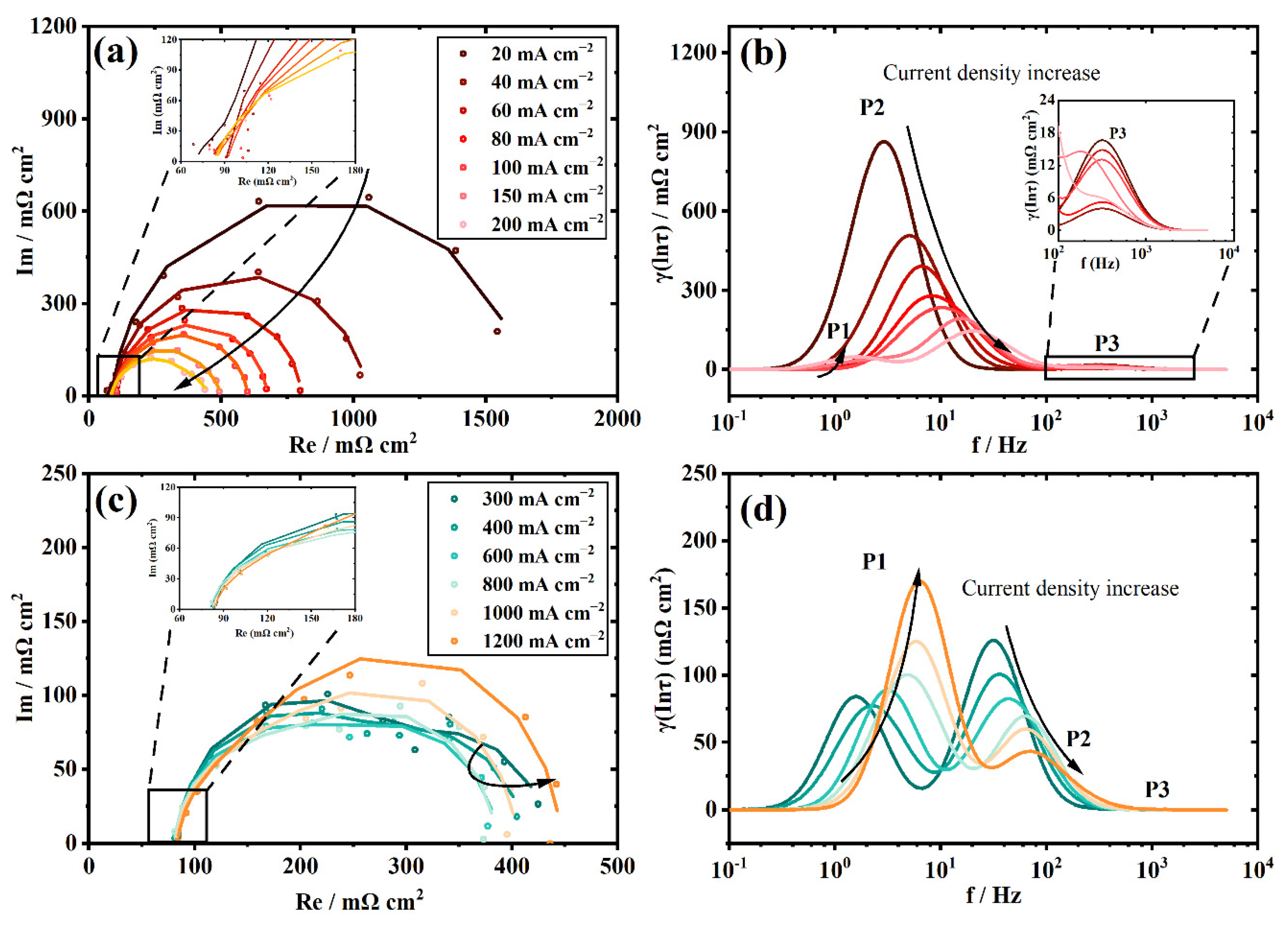
3.2. The Polarization Process Analysis of a New Stack with DRT

In order to analyze the polarization loss variation of the aged stack and further explain the degradation mechanism, it is necessary to use the DRT method to identify the individual polarization processes of the new and aged stacks.

That the polarization curve of the PEMFC is nonlinear reveals an exponential drop at low current densities, a nearly linear drop at medium current densities, and a sharp drop at high current densities. Therefore, the polarization impedance is different in the whole range of current densities. In order to describe the overall behavior of the system, the range of current densities for EIS testing is taken from 20 mA cm⁻² to 1200 mA cm⁻², covering low and high current densities. The other operating conditions are kept constant, according to Table 1.

The Nyquist plots in Figure 5a,c show that the polarization resistance $R_{\mathrm{pol}}$ decreases rapidly from 1529 mΩ cm² to 355 mΩ cm² with the increase in current density at low current density regions (from 20 mA cm⁻² to 200 mA cm⁻²) and decreases gently from 340 mΩ cm² to 294 mΩ cm² at medium current density regions (from 300 mA cm⁻² to 600 mA cm⁻²). However, at high current density regions (from 800 mA cm⁻² to 1200 mA cm⁻²), the polarization resistance $R_{\mathrm{pol}}$ increases slightly from 276 mΩ cm² to 353 mΩ cm² with the increase in current densities. The main reason is that the mass transport limitation gradually dominates.

From the enlarged view of the above figure, the ohmic resistance $R_0$ is almost constant at 80 mΩ cm² over the entire current densities range. In addition, at low current density regions, an obvious arc appears in the high-frequency region of the EIS data, which will be explained in the DRT analysis below.

Figure 5b,d is the DRT spectra under overall current densities. In Figure 5b, the DRT spectra contains three peaks. In the low current density regions (from 20 mA cm⁻² to 200 mA cm⁻²), the P2 peak dominates the polarization process and rapidly decreases, and the characteristic frequency gradually shifts right from 3 Hz (20 mA cm⁻²) to 20 Hz (200 mA cm⁻²) with the increase in current density. In the enlarged view of Figure 5b, there is a P3 peak in the high-frequency region next to the P2 peak. The P3 peak has almost no correlation with the current density, and the characteristic frequency is about 300 Hz. The peak P3 in the high-frequency region is related to the process of the anode side and the proton transport of the cathode catalyst layer [23,35]. Due to the small peak of P3, the contribution for the polarization loss analysis can be ignored. The P1 peak begins to appear and the characteristic frequency is about 1.3 Hz (200 mA cm⁻²) in the low-frequency region left to peak P2.

In Figure 5d, in the middle and high current density regions (from 300 mA cm⁻² to 1200 mA cm⁻²), the P2 peak decreases slowly with the increase in current density, and the characteristic frequency continuously shifts right to 70 Hz (1200 mA cm⁻²). Due to the right shift of the P2 peak, the characteristics of the P3 peak are rolled inside the P2 peak; therefore, the P3 peak almost disappears in the high current density region. This phenomenon can also be verified from the high-frequency region of the Nyquist plot which has an obvious arc at the low current density region but disappears at the high current density region. With the increase in current density, the P1 peak gradually rises and dominates the polarization process. The characteristic frequency of P1 gradually shifts to the right of 6.5 Hz (1200 mA cm⁻²). The shift in the characteristic frequency of P1 is mainly due to the decrease in the polarization resistance.

From the above analysis, the strongly dependent relationship between the P2 peak and current density are highly consistent with the charge transfer impedance of oxygen reduction reactions (ORRs), and the charge transfer impedance also dominates the polarization loss in the low current density regions [54,55].

In previous studies [35,36], the P1 peak attributed to the cathode oxygen mass transport impedance was obtained by EIS testing under pure oxygen conditions in which the P1 peak almost disappeared. In order to further verify the relationship between the cathode oxygen mass transport and the P1 peak, the EIS tests changed the air stoichiometry at the high current density (800 mA cm⁻²) from 2.3 to 1.4 (the other operating conditions refer to

Table 3. The resistance values of the new and aged stacks at different current densities.

Current Density	Type	New Stack	Aged Stack	Growth Rate
60 mA cm−2	$R_{\mathrm{ct}}$	693 mΩ cm2	854 mΩ cm2	23%
	$R_{\mathrm{diff}}$	0	0	-
	$R_{\mathrm{ohm}}$	81.5 mΩ cm2	104 mΩ cm2	22%
	$R_{\mathrm{an}}$	24.3 mΩ cm2	6 mΩ cm2	−75%
200 mA cm−2	$R_{\mathrm{ct}}$	292 mΩ cm2	372 mΩ cm2	27%
	$R_{\mathrm{diff}}$	78 mΩ cm2	105 mΩ cm2	35%
	$R_{\mathrm{ohm}}$	84.8 mΩ cm2	90 mΩ cm2	6%
	$R_{\mathrm{an}}$	4.7 mΩ cm2	0	-
400 mA cm−2	$R_{\mathrm{ct}}$	183 mΩ cm2	220 mΩ cm2	20%
	$R_{\mathrm{diff}}$	146 mΩ cm2	195 mΩ cm2	34%
	$R_{\mathrm{ohm}}$	83 mΩ cm2	85.4 mΩ cm2	3%
	$R_{\mathrm{an}}$	0	0	-
800 mA cm−2	$R_{\mathrm{ct}}$	109 mΩ cm2	139 mΩ cm2	28%
	$R_{\mathrm{diff}}$	190 mΩ cm2	254 mΩ cm2	34%
	$R_{\mathrm{ohm}}$	82 mΩ cm2	86 mΩ cm2	4%
	$R_{\mathrm{an}}$	0	0	-

). According to the Nyquist plot in Figure 6a, as the air stoichiometry gradually decreases, the right arc gradually increases. It can be seen more clearly from the DRT spectrum in Figure 6b that the P1 peak is also gradually increasing. This conclusion is consistent with the air stoichiometry mainly affecting the cathode mass transport under high current density [56].

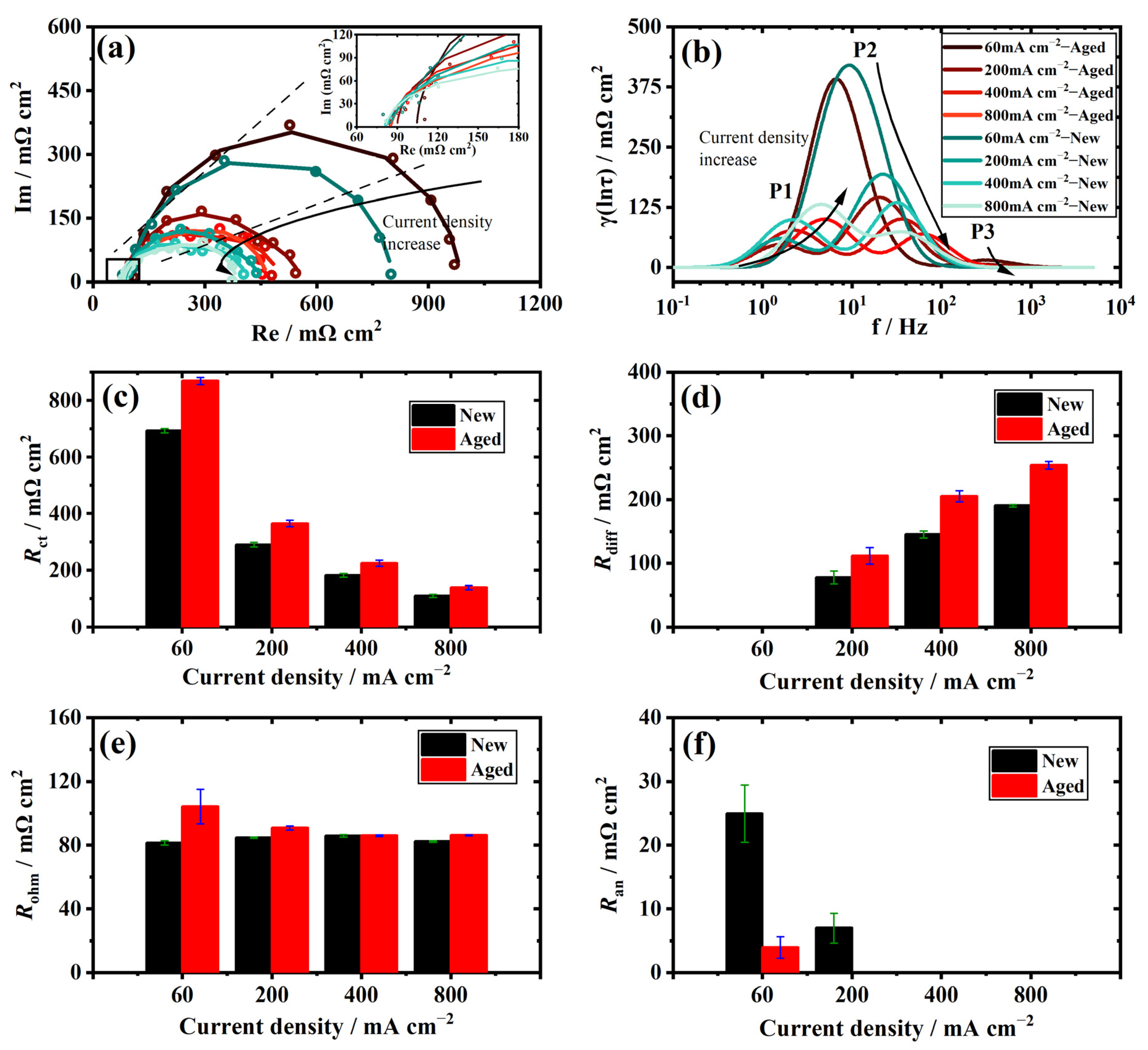
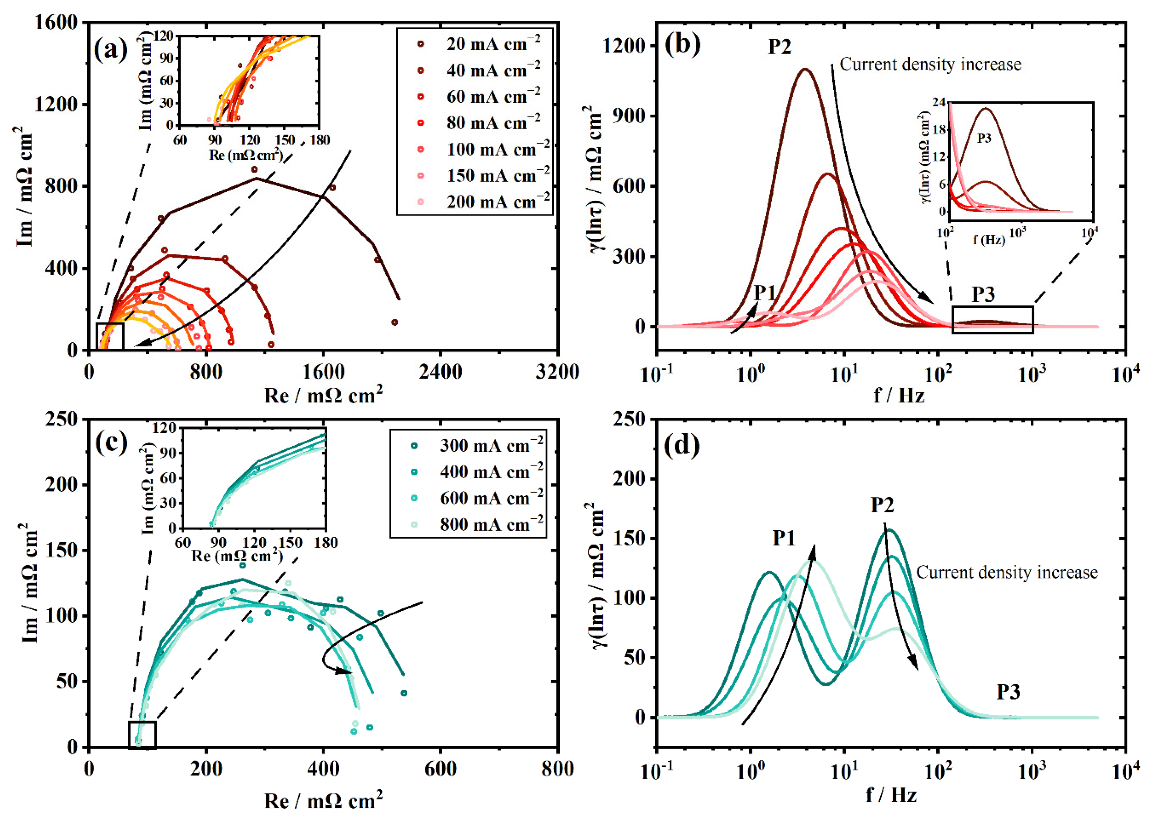
3.3. The Polarization Process Analysis of the Aged Stack with DRT

The aged stack had run for above 2000 h on the bus and the equivalent driving cycle is shown in Figure 7a. The total driving cycle time is 500 min, and the main operating points are 30% (240 mA cm⁻²), 50% (400 mA cm⁻²), and 100% (800 mA cm⁻²) rated power. After that, the polarization curve of the aged stack is shown in Figure 7. Compared with the new stack, the voltage of the aged stack decreases significantly at each current density point. As can be seen from the I–V polarization curve, the voltage has been reduced from 0.89 V to 0.85 V even at a low current density (20 mA cm⁻²). The voltage recession also increases gradually with the increase in current density. The voltage is reduced from 0.67 V to 0.57 V at the rated current density of 800 mA cm⁻² with a recession rate of 15%. Furthermore, the voltage data of the stack at 100% rated power (800 mA cm⁻²) is extracted, and the average voltage of the stack at this operating point per day is used as the average cell voltage ${\overline{V}}_{\mathrm{cell}}$. The curve of ${\overline{V}}_{\mathrm{cell}}$ at 800 mA cm⁻² during the driving cycle is shown in Figure 7c. ${\overline{V}}_{\mathrm{cell}}$ gradually decreases from 0.65 V to 0.57 V. In the first 120 days, ${\overline{V}}_{\mathrm{cell}}$ undergoes large fluctuations but the overall decline is slight. This abnormal fluctuation is mainly due to the unsuitability of the operating conditions of the stack caused by the change in ambient temperature. For example, the capacity of the air compressor will decrease with an increase in ambient temperature, resulting in water management problems for the stack. After 120 days, ${\overline{V}}_{\mathrm{cell}}$ gradually decreases from 0.64 V to 0.57 V, and the ${\overline{V}}_{\mathrm{cell}}$ reaches its lowest point at 240 days. The EIS tests are carried out at 240 days.

Due to the severe decay of the aged stack, it is difficult to operate stably for a long time under large current density regions. Therefore, the EIS data testing range is taken from 20 mA cm⁻² to 800 mA cm⁻². The other operating conditions are kept constant, according to Table 2.

The Nyquist plots from Figure 8a,c show that the polarization resistance $R_{\mathrm{pol}}$ decreases rapidly from 2220 mΩ cm² to 450 mΩ cm² with the increase in current density at low current density regions (from 20 mA cm⁻² to 300 mA cm⁻²); however, it remains constant at 410 mΩ cm² in the middle and high current density regions (from 400 mA cm⁻² to 800 mA cm⁻²). The polarization resistance $R_{\mathrm{pol}}$ increases by 48% compared with the new stack at 800 mA cm⁻².

From the enlarged view of the above figure, it can be seen that the ohmic resistance $R_0$ slightly drops from 115 mΩ cm² to 90 mΩ cm² in the low current density regions and remains almost constant at 90 mΩ cm² in the high current density region. The ohmic resistance $R_{\mathrm{o}}$ increases by 4% compared with the new stack at 800 mA cm⁻² (Table 3).

In Figure 8b, in the low current density regions, the P2 peak also rapidly decreases and the characteristic frequency gradually shifts right from 3.7 Hz (20 mA cm⁻²) to 21 Hz (200 mA cm⁻²) with the increase in current density. In the enlarged view of Figure 8b, the characteristic frequency of the P3 peak is 310 Hz.

In Figure 8d, in the high current density regions (from 300 mA cm⁻² to 800 mA cm⁻²), the P2 peak decreases slowly with the increase in current density, and the characteristic frequency continuously shifts right to 38 Hz (800 mA cm⁻²). The P3 peak also disappears in the high current density region. With the increase in current density, the P1 peak gradually rises and dominates the polarization process. The characteristic frequency of P1 gradually shifts to the right to 4.7 Hz (800 mA cm⁻²). From the above analysis, the characteristic frequency of the P1 and the P2 peaks has slightly increased, but the distribution function has undergone a significant increase compared with the new stack.

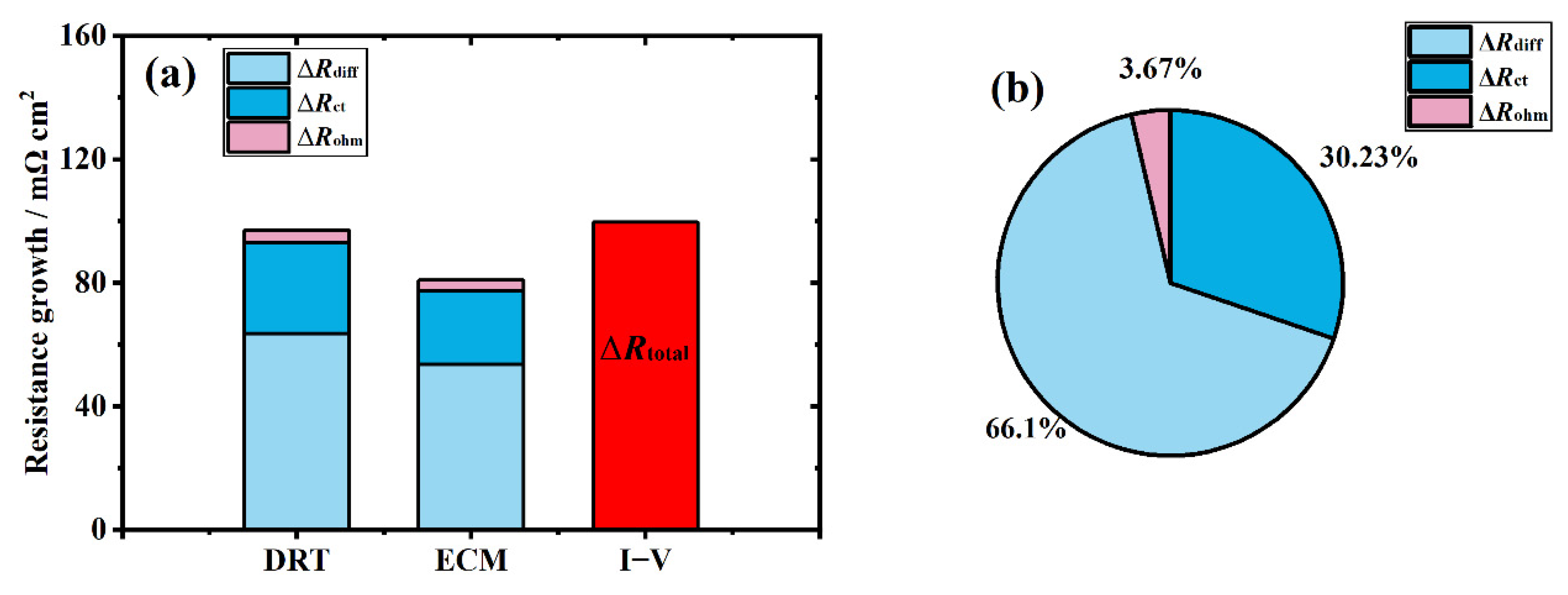
3.4. Individual Resistance Growth of the Aged Stack

The RC element can represent the electrochemical system with distributed parameters and the relevant DRT plot is shown in Figure 9a,b. The impedance of an RC element can be expressed as R/(1 + (jωτ)); τ is the time constant. For the standard RC elements, the area of the peak is proved to be equal to the resistance of the RC element and the time constant τ is equal to the RC. Figure 9c displays the calculated DRT spectrum with a $\lambda$ value of 10⁻³ at the current density of 400 mA cm⁻² for the new stack. There are two obvious peaks, hence a two-order RC ECM is applied and compared with the DRT results in Figure 9c. Each peak region represents an independent polarization process, and the area within the span of each region from $f_l$ to $f_u$ represents the resistance, $R_{\mathrm{pol}-\mathrm{i}},$ of the polarization process [33].

$$R_{\mathrm{pol}-\mathrm{i}}={\int }_{1/(2\pi f_u)}^{1/\left(2\pi f_l\right)}\gamma \left(\ln \left(1/\left(2\pi f\right)\right)\right)d\left(\ln \left(1/\left(2\pi f\right)\right)\right)$$

(11)

The capacitance C can also be calculated by the characteristic frequency f ($C=1/\left(2\pi fR\right)$). Then, the parameters of the two-order RC ECM are fitted using Zview software (Scribner Associates Inc./Southern Pines, NC, USA) with the initial value set by the DRT. Based on the above polarization process analysis and the principle of DRT, the area of the P1 peak represents the cathode oxygen mass transport resistance, $R_{\mathrm{diff}}$; the area of the P2 peak represents the charge transfer resistance, $R_{\mathrm{ct}}$, of ORRs; and the area of the P3 peak represents the sum of the anode chemical reaction resistance and the proton transport resistance of the cathode catalytic layer, $R_{\mathrm{an}}$. The intercept at the real axis of the Nyquist plot in the high-frequency region represents the ohmic resistance, $R_{\mathrm{ohm}}$.

In this paper, the EIS data at four typical current densities are used to comparatively analyze new and aged stacks.

From the Nyquist plot in Figure 10a, the aged stack has a larger arc, which means that the polarization resistance, $R_{\mathrm{pol}},$ is larger. The enlarged view of Figure 10a clearly shows that the ohmic resistance, $R_{\mathrm{ohm}},$ slightly increases. Similarly, from the DRT spectra in Figure 10b, the P1 and P2 peaks of the aged stack are larger, while the characteristic frequency only slightly increases.

Figure 10c–f compares the individual resistance of the new and aged stack respectively. As can be seen from Figure 10c, the $R_{\mathrm{ct}}$ of the aged stack decreases gradually from 854 mΩ cm² to 139 mΩ cm² (from 60 mA cm⁻² to 800 mA cm⁻²). At each current density, the growth rate of $R_{\mathrm{ct}}$ is about 25% compared to the new stack. $R_{\mathrm{diff}}$ is basically 0 at a low current density and increases rapidly from 100 mΩ cm² to 250 mΩ cm² (from 200 mA cm⁻² to 800 mA cm⁻²) in the aged stack (Figure 10d). The growth rate of $R_{\mathrm{diff}}$ of the aged stack compared to the new stack is about 35%. It can be seen from Figure 10e that the $R_{\mathrm{ohm}}$ of the aged stack slightly increases compared with that of the new stack. The growth rate is about 5%. However, the growth rate is larger at a low current density, possibly because the gas humidity of the aged stack does not completely reach the preset humidity range. It can be seen from Figure 10f that the resistance value of $R_{\mathrm{an}}$ is relatively small and only exists in low current density regions. The growth rate of $R_{\mathrm{an}}$ is negative in the low current density range and $R_{\mathrm{an}}$ even disappears in the middle and high current density regions. This anomaly may be due to the fact that the characteristic frequency of the P2 peak of the aged stack is shifted to the right compared to the new stack. The P3 peak is more affected by the P2 peak and is rolled inside the P2 peak at a smaller current density, resulting in a decrease in the area of the P3 peak. With the increase in current density, the P2 peak shifts more to the right, resulting in the disappearance of the P3 peak. However, the P3 peak is relatively small and can be ignored without affecting the accuracy of the calculation. The resistance values of the new and aged stacks at different current densities are shown in Table 3.

3.5. Recession Analysis of the Aged Stack

In order to verify the accuracy of the resistance growth in each polarization process decomposed by the DRT method in the analysis of the decay process of the aged stack, the resistance growth decomposed by the ECM of the measured EIS data and the equivalent resistance growth in the I–V polarization curve at the rated current density of 800 mA cm⁻² are compared. As can be seen from Figure 11a, the sum of the resistance growth of each polarization process decomposed by DRT is 97 mΩ cm², the resistance growth analyzed by the ECM of the measured EIS data is 89 mΩ cm², and the equivalent resistance growth of the voltage decrease through the I–V polarization curve $\Delta R_{\mathrm{total}}$ is 99 mΩ cm². The DRT method is closer to the actual resistance growth, and the deviation is about 3%. Therefore, it can be considered that the DRT method is effective in the analysis of the aged stack.

Figure 11b shows the proportion of different polarization resistance growths at the rated current density of 800 mA cm⁻². In Figure 11b, $\Delta R_{\mathrm{diff}}$ overwhelmingly dominates the resistance growth of 66.1%, which means that the oxygen mass transport performance of the aged stack undergoes a severe decline and the possible influencing factors include the GDL/MPL and the catalyst layer (CL). The low temperatures at which the PEMFC operates mean that the product water is almost liquid. This liquid water can accumulate in the pores of the CL and must be removed to keep the gas pathways to the active sites of the CL unblocked [57]. Many researchers have reported that the GDL interacts with the changes in water during durability tests. These changes appear to occur at the microstructural level [58,59]. The GDL gradually changes from hydrophobic to hydrophilic and gas diffusion and convection are blocked after the durability test [60]. In addition, liquid water covers the catalyst–ionomer phase in the CL, limiting the flow of gas to the active platinum sites [61]. As a result, the performance of the PEMFC decreases drastically under high current densities. Keeping the hydrophobic properties of the GDL/MPL hydrophobic gradient constant is important for maintaining mass transport during the durability test. $\Delta R_{\mathrm{ct}}$ also makes a great contribution to the resistance growth of 30.23%. Carbon corrosion and the dissolution and aggregation of platinum catalysts may be the main reasons for the increase in ORR polarization resistance [1,14,17,62]. $\Delta R_{\mathrm{ohm}}$ has little effect on resistance growth, which is only 3.67%.

4. Conclusions

In this work, the quantitative DRT method has been successfully applied to analyze the aged vehicular PEMFC stack by running a driving cycle for 2000 h. After 2000 h operation on the bus, the performance of the stack deteriorates seriously, and the rated power at 800 mA cm⁻² declines by about 15%. The resistance growth method based on the DRT is proposed to determine the reason for the decline of the stack.

Firstly, the peaks in the DRT spectra representing the individual polarization process are verified by changing the air stoichiometry and the current density. The P1 peak in the low-frequency region (3 Hz) gradually increases with the decrease in air stoichiometry, which represents oxygen mass transport impedance. The P2 peak in the middle frequency region (20 Hz) decreases exponentially as the current density increases, which represents the charge transfer impedance of the ORRs. The P3 peak in the high-frequency region (300 Hz) is almost unaffected by current density, which represents the impedance of proton transfer in the CCL and anode side. The area of the P3 peak is almost negligible and rolled inside the P2 peak in the high current density region. The high-frequency intercept of the Nyquist plot represents the ohmic resistance.

The impedance of each polarization process is calculated quantitatively by each corresponding peak area and its influence on power decline is analyzed. By calculating the polarization resistance and ohmic resistance of the new and aged stack, the resistance growth of the aged stack is given. The resistance growths obtained by the DRT, ECM, and I–V of the aged stack at a rated current density of 800 mA cm⁻² were compared to verify the accuracy of the DRT method. The DRT method has been found to yield a result closer to the actual resistance growth, with a deviation of about 3%, which verifies the effectiveness of the DRT method. The increase in mass transport resistance is the main reason for the resistance growth, accounting for 66.1% at rated power. We believe that optimizing the oxygen mass transport performance is the key factor in improving the lifetime of the stack. The charge transfer resistance of the ORRs also makes a great contribution to the resistance growth of 30.23% at rated power. The ohmic resistance has little effect on resistance growth.

Therefore, the DRT method can quickly and accurately separate the individual polarization process from the EIS data, with no need to establish a complex mechanism model or an ECM. It is therefore expected to become an important diagnostic tool for PEMFC aging.

References

1. Shan, J.; Lin, R.; Xia, S.; Liu, D.; Zhang, Q. Local resolved investigation of PEMFC performance degradation mechanism during dynamic driving cycle. Int. J. Hydrog. Energy 2016, 41, 4239–4250. [Google Scholar] [CrossRef]
2. Pei, P.; Chen, H. Main factors affecting the lifetime of Proton Exchange Membrane fuel cells in vehicle applications: A review. Appl. Energy 2014, 125, 60–75. [Google Scholar] [CrossRef]
3. Yu, Y.; Tu, Z.; Zhang, H.; Zhan, Z.; Pan, M. Comparison of degradation behaviors for open-ended and closed proton exchange membrane fuel cells during startup and shutdown cycles. J. Power Sources 2011, 196, 5077–5083. [Google Scholar] [CrossRef]
4. Al Amerl, A.; Oukkacha, I.; Camara, M.B.; Dakyo, B. Real-Time Control Strategy of Fuel Cell and Battery System for Electric Hybrid Boat Application. Sustainability 2021, 13, 8693. [Google Scholar] [CrossRef]
5. Hu, D.; Wang, Y.; Li, J.; Yang, Q.; Wang, J. Investigation of optimal operating temperature for the PEMFC and its tracking control for energy saving in vehicle applications. Energy Convers Manag. 2021, 249, 114842. [Google Scholar] [CrossRef]
6. Shen, J.; Xu, L.; Chang, H.; Tu, Z.; Chan, S.H. Partial flooding and its effect on the performance of a proton exchange membrane fuel cell. Energy Convers Manag. 2020, 207, 112537. [Google Scholar] [CrossRef]
7. Ozden, A.; Shahgaldi, S.; Li, X.; Hamdullahpur, F. The impact of ionomer type on the morphological and microstructural degradations of proton exchange membrane fuel cell electrodes under freeze-thaw cycles. Appl. Energy 2019, 238, 1048–1059. [Google Scholar] [CrossRef]
8. Yu, Y.; Li, H.; Wang, H.J.; Yuan, X.Z.; Wang, G.J.; Pan, M. A review on performance degradation of proton exchange membrane fuel cells during startup and shutdown processes: Causes, consequences, and mitigation strategies. J. Power Sources 2012, 205, 10–23. [Google Scholar] [CrossRef] [Green Version]
9. Bose, A.; Babburi, P.; Kumar, R.; Myers, D.; Mawdsley, J.; Milhuff, J. Performance of individual cells in polymer electrolyte membrane fuel cell stack under-load cycling conditions. J. Power Sources 2013, 243, 964–972. [Google Scholar] [CrossRef]
10. Ren, P.; Pei, P.; Li, Y.; Wu, Z.; Chen, D.; Huang, S. Degradation mechanisms of proton exchange membrane fuel cell under typical automotive operating conditions. Prog. Energy Combust. Sci. 2020, 80, 100859. [Google Scholar] [CrossRef]
11. Galbiati, S.; Baricci, A.; Casalegno, A.; Marchesi, R. Degradation in phosphoric acid doped polymer fuel cells: A 6000 h parametric investigation. Int. J. Hydrog. Energy 2013, 38, 6469–6480. [Google Scholar] [CrossRef]
12. Kim, J.-R.; Yi, J.S.; Song, T.-W. Investigation of degradation mechanisms of a high-temperature polymer-electrolyte-membrane fuel cell stack by electrochemical impedance spectroscopy. J. Power Sources 2012, 220, 54–64. [Google Scholar] [CrossRef]
13. Lee, K.-S.; Lee, B.-S.; Yoo, S.J.; Kim, S.-K.; Hwang, S.J.; Kim, H.-J.; Cho, E.; Henkensmeier, D.; Yun, J.W.; Nam, S.W.; et al. Development of a galvanostatic analysis technique as an in-situ diagnostic tool for PEMFC single cells and stacks. Int. J. Hydrog. Energy 2012, 37, 5891–5900. [Google Scholar] [CrossRef]
14. Gazdzick, P.; Mitzel, J.; Garcia Sanchez, D.; Schulze, M.; Friedrich, K.A. Evaluation of reversible and irreversible degradation rates of polymer electrolyte membrane fuel cells tested in automotive conditions. J. Power Sources 2016, 327, 86–95. [Google Scholar] [CrossRef] [Green Version]
15. Cadet, C.; Jemeï, S.; Druart, F.; Hissel, D. Diagnostic tools for PEMFCs: From conception to implementation. Int. J. Hydrog. Energy 2014, 39, 10613–10626. [Google Scholar] [CrossRef]
16. Zhang, X.; Zhang, T.; Chen, H.; Cao, Y. A review of online electrochemical diagnostic methods of on-board proton exchange membrane fuel cells. Appl. Energy 2021, 286, 116481. [Google Scholar] [CrossRef]
17. Pavlisic, A.; Jovanovic, P.; Selih, V.S.; Sala, M.; Hodnik, N.; Gaberscek, M. Platinum Dissolution and Redeposition from Pt/C Fuel Cell Electrocatalyst at Potential Cycling. J. Electrochem. Soc. 2018, 165, F3161–F3165. [Google Scholar] [CrossRef]
18. Ma, T.; Zhang, Z.; Lin, W.; Cong, M.; Yang, Y. Impedance prediction model based on convolutional neural networks methodology for proton exchange membrane fuel cell. Int. J. Hydrog. Energy 2021, 46, 18534–18545. [Google Scholar] [CrossRef]
19. Rezaei Niya, S.M.; Hoorfar, M. Study of proton exchange membrane fuel cells using electrochemical impedance spectroscopy technique—A review. J. Power Sources 2013, 240, 281–293. [Google Scholar] [CrossRef]
20. Tang, Z.; Huang, Q.-A.; Wang, Y.-J.; Zhang, F.; Li, W.; Li, A.; Zhang, L.; Zhang, J. Recent progress in the use of electrochemical impedance spectroscopy for the measurement, monitoring, diagnosis and optimization of proton exchange membrane fuel cell performance. J. Power Sources 2020, 468, 228361. [Google Scholar] [CrossRef]
21. Ma, T.; Lin, W.; Zhang, Z.; Kang, J.; Yang, Y. Research on electrochemical impedance spectroscope behavior of fuel cell stack under different reactant relative humidity. Int. J. Hydrog. Energy 2021, 46, 17388–17396. [Google Scholar] [CrossRef]
22. Lu, H.; Chen, J.; Yan, C.; Liu, H. On-line fault diagnosis for proton exchange membrane fuel cells based on a fast electrochemical impedance spectroscopy measurement. J. Power Sources 2019, 430, 233–243. [Google Scholar] [CrossRef]
23. Yuan, H.; Dai, H.; Wei, X.; Ming, P. Internal polarization process revelation of electrochemical impedance spectroscopy of proton exchange membrane fuel cell by an impedance dimension model and distribution of relaxation times. Chem. Eng. J. 2021, 418, 129358. [Google Scholar] [CrossRef]
24. Rezaei Niya, S.M.; Phillips, R.K.; Hoorfar, M. Process modeling of the impedance characteristics of proton exchange membrane fuel cells. Electrochim. Acta 2016, 191, 594–605. [Google Scholar] [CrossRef] [Green Version]
25. Danzer, M.A.; Hofer, E.P. Analysis of the electrochemical behaviour of polymer electrolyte fuel cells using simple impedance models. J. Power Sources 2009, 190, 25–33. [Google Scholar] [CrossRef]
26. Dhirde, A.M.; Dale, N.V.; Salehfar, H.; Mann, M.D.; Han, T. Equivalent Electric Circuit Modeling and Performance Analysis of a PEM Fuel Cell Stack Using Impedance Spectroscopy. IEEE Trans. Energy Convers. 2010, 25, 778–786. [Google Scholar] [CrossRef]
27. Macdonald, D.D. Reflections on the history of electrochemical impedance spectroscopy. Electrochim. Acta 2006, 51, 1376–1388. [Google Scholar] [CrossRef]
28. Huang, J.; Li, Z.; Liaw, B.Y.; Zhang, J. Graphical analysis of electrochemical impedance spectroscopy data in Bode and Nyquist representations. J. Power Sources 2016, 309, 82–98. [Google Scholar] [CrossRef]
29. Leonide, A.; Apel, Y.; Ivers-Tiffee, E. SOFC Modeling and Parameter Identification by Means of Impedance Spectroscopy. ECS Trans. 2009, 19, 81–109. [Google Scholar] [CrossRef]
30. Leonide, A.; Sonn, V.; Weber, A.; Ivers-Tiffee, E. Evaluation and Modelling of the Cell Resistance in Anode Supported Solid Oxide Fuel Cells. ECS Trans. 2007, 7, 521–531. [Google Scholar] [CrossRef]
31. Ivers-Tiffee, E.; Weber, A. Evaluation of electrochemical impedance spectra by the distribution of relaxation times. J. Ceram. Soc. Jpn. 2017, 125, 193–201. [Google Scholar] [CrossRef] [Green Version]
32. Guo, D.; Yang, G.; Zhao, G.; Yi, M.; Feng, X.; Han, X.; Lu, L.; Ouyang, M. Determination of the Differential Capacity of Lithium-Ion Batteries by the Deconvolution of Electrochemical Impedance Spectra. Energies 2020, 13, 915. [Google Scholar] [CrossRef] [Green Version]
33. Zhou, X.; Huang, J.; Pan, Z.; Ouyang, M. Impedance characterization of lithium-ion batteries aging under high-temperature cycling: Importance of electrolyte-phase diffusion. J. Power Sources 2019, 426, 216–222. [Google Scholar] [CrossRef]
34. Kulikovsky, A. PEM fuel cell distribution of relaxation times: A method for the calculation and behavior of an oxygen transport peak. Phys. Chem. Chem. Phys. 2020, 22, 19131–19138. [Google Scholar] [CrossRef]
35. Heinzmann, M.; Weber, A.; Ivers-Tiffée, E. Advanced impedance study of polymer electrolyte membrane single cells by means of distribution of relaxation times. J. Power Sources 2018, 402, 24–33. [Google Scholar] [CrossRef]
36. Weiß, A.; Schindler, S.; Galbiati, S.; Danzer, M.A.; Zeis, R. Distribution of Relaxation Times Analysis of High-Temperature PEM Fuel Cell Impedance Spectra. Electrochim. Acta 2017, 230, 391–398. [Google Scholar] [CrossRef]
37. Boukamp, B.A. A Linear Kronig-Kramers Transform Test for Immittance Data Validation. J. Electrochem. Soc. 1995, 142, 1885–1894. [Google Scholar] [CrossRef]
38. Agarwal, P.; Crisalle, O.D.; Orazem, M.E.; Garcia-Rubio, L.H. Application of Measurement Models to Impedance Spectroscopy: II Determination of the Stochastic Contribution to the Error Structure. J. Electrochem. Soc. 1995, 142, 4149–4158. [Google Scholar] [CrossRef]
39. Schönleber, M.; Ivers-Tiffée, E. Approximability of impedance spectra by RC elements and implications for impedance analysis. Electrochem. Commun. 2015, 58, 15–19. [Google Scholar] [CrossRef]
40. Schönleber, M.; Klotz, D.; Ivers-Tiffée, E. A Method for Improving the Robustness of linear Kramers-Kronig Validity Tests. Electrochim. Acta 2014, 131, 20–27. [Google Scholar] [CrossRef]
41. Saccoccio, M.; Wan, T.H.; Chen, C.; Ciucci, F. Optimal Regularization in Distribution of Relaxation Times applied to Electrochemical Impedance Spectroscopy: Ridge and Lasso Regression Methods—A Theoretical and Experimental Study. Electrochim. Acta 2014, 147, 470–482. [Google Scholar] [CrossRef]
42. Boukamp, B.A.; Rolle, A. Analysis and Application of Distribution of Relaxation Times in Solid State Ionics. Solid State Ion. 2017, 302, 12–18. [Google Scholar] [CrossRef]
43. Boukamp, B.A. Fourier transform distribution function of relaxation times; application and limitations. Electrochim. Acta 2015, 154, 35–46. [Google Scholar] [CrossRef]
44. Horlin, T. Deconvolution and maximum entropy in impedance spectroscopy of noninductive systems. Solid State Ion. 1998, 107, 241–253. [Google Scholar] [CrossRef]
45. Zhang, Y.; Chen, Y.; Li, M.; Yan, M.; Ni, M.; Xia, C. A high-precision approach to reconstruct distribution of relaxation times from electrochemical impedance spectroscopy. J. Power Sources 2016, 308, 1–6. [Google Scholar] [CrossRef]
46. Ciucci, F.; Chen, C. Analysis of Electrochemical Impedance Spectroscopy Data Using the Distribution of Relaxation Times: A Bayesian and Hierarchical Bayesian Approach. Electrochim. Acta 2015, 167, 439–454. [Google Scholar] [CrossRef]
47. Wan, T.H.; Saccoccio, M.; Chen, C.; Ciucci, F. Influence of the Discretization Methods on the Distribution of Relaxation Times Deconvolution: Implementing Radial Basis Functions with DRTtools. Electrochim. Acta 2015, 184, 483–499. [Google Scholar] [CrossRef]
48. Tuncer, E.; Gubanski, S.M. On dielectric data analysis—Using the Monte Carlo method to obtain relaxation time distribution and comparing non-linear spectral function fits. IEEE Trans. Dielectr. Electr. Insul. 2001, 8, 310–320. [Google Scholar] [CrossRef]
49. Tesler, A.B.; Lewin, D.R.; Baltianski, S.; Tsur, Y. Analyzing results of impedance spectroscopy using novel evolutionary programming techniques. J. Electroceram. 2009, 24, 245–260. [Google Scholar] [CrossRef]
50. Schlüter, N.; Ernst, S.; Schröder, U. Finding the Optimal Regularization Parameter in Distribution of Relaxation Times Analysis. ChemElectroChem 2019, 6, 6027–6037. [Google Scholar] [CrossRef] [Green Version]
51. Setzler, B.P.; Fuller, T.F. A Physics-Based Impedance Model of Proton Exchange Membrane Fuel Cells Exhibiting Low-Frequency Inductive Loops. J. Electrochem. Soc. 2015, 162, F519–F530. [Google Scholar] [CrossRef]
52. Roy, S.K.; Orazem, M.E.; Tribollet, B. Interpretation of Low-Frequency Inductive Loops in PEM Fuel Cells. J. Electrochem. Soc. 2007, 154, B1378. [Google Scholar] [CrossRef]
53. Schiefer, A.; Heinzmann, M.; Weber, A. Inductive Low-Frequency Processes in PEMFC-Impedance Spectra. Fuel Cells 2020, 20, 499–506. [Google Scholar] [CrossRef] [Green Version]
54. Kulikovsky, A.A. PEM Fuel Cell Impedance at Open Circuit. J. Electrochem. Soc. 2016, 163, F319–F326. [Google Scholar] [CrossRef] [Green Version]
55. Kulikovsky, A.A.; Eikerling, M. Analytical solutions for impedance of the cathode catalyst layer in PEM fuel cell: Layer parameters from impedance spectrum without fitting. J. Electroanal. Chem. 2013, 691, 13–17. [Google Scholar] [CrossRef]
56. Kim, B.; Cha, D.; Kim, Y. The effects of air stoichiometry and air excess ratio on the transient response of a PEMFC under load change conditions. Appl. Energy 2015, 138, 143–149. [Google Scholar] [CrossRef]
57. Niblett, D.; Niasar, V.; Holmes, S. Enhancing the Performance of Fuel Cell Gas Diffusion Layers Using Ordered Microstructural Design. J. Electrochem. Soc. 2019, 167, 013520. [Google Scholar] [CrossRef] [Green Version]
58. Liu, D.; Case, S. Durability study of proton exchange membrane fuel cells under dynamic testing conditions with cyclic current profile. J. Power Sources 2006, 162, 521–531. [Google Scholar] [CrossRef]
59. Wood, D.; Davey, J.; Atanassov, P.; Borup, R. PEMFC Component Characterization and Its Relationship to Mass-Transport Overpotentials during Long-Term Testing. ECS Trans. 2006, 3, 753–763. [Google Scholar] [CrossRef]
60. Williams, M.V.; Kunz, H.R.; Fenton, J.M. Influence of Convection Through Gas-Diffusion Layers on Limiting Current in PEM FCs Using a Serpentine Flow Field. J. Electrochem. Soc. 2004, 151, A1617. [Google Scholar] [CrossRef]
61. Yuan, H.; Dai, H.; Ming, P.; Zhao, L.; Tang, W.; Wei, X. Understanding dynamic behavior of proton exchange membrane fuel cell in the view of internal dynamics based on impedance. Chem. Eng. J. 2022, 431, 134035. [Google Scholar] [CrossRef]
62. Ma, T.; Zhu, D.; Xie, J.; Lin, W.; Yang, Y. Investigation on a parking control strategy for automotive proton exchange membrane fuel cell. Fuel Cells 2021, 21, 390–397. [Google Scholar] [CrossRef]
Figure 1. Illustration of the main idea and the analysis procedure.
Sustainability 14 05677 g001
Figure 2. Illustration of the self-made AC impedance equipment.
Sustainability 14 05677 g002
Figure 3. (a) Nyquist plot of EIS data at a current density of 400 mA cm−2 of a new stack. (b) Relative residual of the KK transformation.
Sustainability 14 05677 g003
Figure 4. (a) Calculated DRTs with λ values from 10−1 to 10−4. (b) Relative residual of the real part of the impedance. (c) Relative residual of the imaginary part of the impedance. (d) SSR of the calculated DRT with a λ value from 101 to 10−7.
Sustainability 14 05677 g004
Figure 5. (a) Nyquist plot of low current densities of the new stack. (b) Relevant DRT spectra. (c) Nyquist plot of middle and high current densities of the new stack. (d) Relevant DRT spectra.
Sustainability 14 05677 g005
Figure 6. (a) Nyquist plot with different air stoichiometries from 1.4 to 2.3 (800 mA cm−2). (b) Relevant DRT spectra.
Sustainability 14 05677 g006
Figure 7. (a) The drive cycle of the stack on the bus. (b) The polarization curve of the new and aged stacks. (c) The average cell voltage of 800 mA cm−2 during the driving cycle.
Sustainability 14 05677 g007
Figure 8. (a) Nyquist plot of low current densities of the aged stack. (b) Relevant DRT spectra. (c) Nyquist plot of middle and high current densities of the aged stack. (d) Relevant DRT spectra.
Sustainability 14 05677 g008
Figure 9. (a) ECM for standard RC elements. (b) DRT spectra for standard RC elements. (c) ECM developed by DRT with a λ value of 10−3.
Sustainability 14 05677 g009
Figure 10. (a) Nyquist plot of the new and aged stacks at different current densities. (b) Relevant DRT spectra. (c) Relevant R ct . (d) Relevant R diff . (e) Relevant R ohm . (f) Relevant R an .
Sustainability 14 05677 g010
Figure 11. (a) The resistance growth obtained by the DRT, ECM and I–V of the aged stack at a rated current density of 800 mA cm−2. (b) Relevant proportions of each polarization resistance growth obtained by the DRT.
Sustainability 14 05677 g011