Quantifying the Effects of Stand and Climate Variables on Biomass of Larch Plantations Using Random Forests and National Forest Inventory Data in North and Northeast China

Abstract

The accurate estimation of forest biomass is crucial for supporting climate change mitigation efforts such as sustainable forest management. Although traditional regression models have been widely used to link stand biomass with biotic and abiotic predictors, this approach has several disadvantages, including the difficulty in dealing with data autocorrelation, model selection, and convergence. While machine learning can overcome these challenges, the application remains limited, particularly at a large scale with consideration of climate variables. This study used the random forests (RF) algorithm to estimate stand aboveground biomass (AGB) and total biomass (TB) of larch (Larix spp.) plantations in north and northeast China and quantified the contributions of different predictors. The data for modelling biomass were collected from 445 sample plots of the National Forest Inventory (NFI). A total of 22 independent variables (6 stand and 16 climate variables) were used to develop and train climate-sensitive stand biomass models. Optimization of hyper parameters was implemented using grid search and 10-fold cross-validation. The coefficient of determination (R²) and root mean square error (RMSE) of the RF models were 0.9845 and 3.8008 t ha⁻¹ for AGB, and 0.9836 and 5.1963 t ha⁻¹ for TB. The cumulative contributions of stand and climate factors to stand biomass were >98% and <2%, respectively. The most crucial stand and climate variables were stand volume and annual heat-moisture index (AHM), with relative importance values of >60% and ~0.25%, respectively. The partial dependence plots illustrated the complicated relationships between climate factors and stand biomass. This study illustrated the power of RF for estimating stand biomass and understanding the effects of stand and climate factors on forest biomass. The application of RF can be useful for mapping of large-scale carbon stock.

1. Introduction

Forests play a vital role in mitigating climate change by absorbing CO₂ and storing it in biomass, with the global forest ecosystem holding ~861 ± 66 Gt of carbon reserves [1]. Therefore, forests provide effective global climate regulation services [2]. Accurately estimating forest biomass and quantifying the effects of biotic and abiotic factors are particularly important. Regression models are widely applied to represent the relationships between forest biomass and independent variables. Stand biomass is usually expressed as a function of stand variables such as stand average diameter at breast height (1.3 m), volume, density, and age [3,4,5,6,7,8,9,10,11]. For example, Bi et al. [4] predicted the stand biomass of Pinus radiata plantations by stand age, basal area, average height of the 50 largest diameter trees, and stand density. Forest biomass was also influenced by meteorological variables, therefore, climate-sensitive individual tree biomass models have been recently developed [12,13,14,15,16]. The application of these models had shown that climate has a significant impact on biomass and that these models produce more accurate predictions [17,18]. Usoltsev et al. [19] showed that an increase in temperature of 1℃ and an increase in precipitation of 100 mm would lead to an increase and decrease in the biomass of stands of Pinus sp. aged 100 years of 2.2% and 5.8%, respectively. However, a similar study showed that the stand biomass of Birch increased with increasing rainfall and mean winter temperature [20]. He et al. [21] developed a climate-sensitive stand biomass model for estimating forest biomass based on traditional simultaneous equations. Their study found that consideration of the climate effect within application of the model resulted in a 411,549 Mg biomass difference in large-scale larch plantations region with the area of 3,085,400 ha. However, there were much uncertainty on the results of impacts of climate on stand biomass. Previous studies have collected data with small samples [22,23] and small-scale experimental sites [5,6,8,24], and a single predictor has usually been selected to estimate stand biomass [6].

Regression models are a powerful tool for understanding the contributions of different factors to stand biomass. However, stand survey data are hierarchical and autocorrelated in space and time, thus the assumptions of the error term normally distributed, independent, and homoscedastic are usually difficult to satisfy [25,26,27]. In addition, an increase in the number of independent variables complicates the regression relationship. A specific mathematical equation needs to be chosen for each independent variable resulting in model selection experiments [5,6]. Furthermore, the convergence of the iterative process used for estimating model parameters cannot be guaranteed. These challenges have resulted in difficulties in the application of traditional statistical models.

Non-parametric methods, such as machine learning (ML), have also shown great potential for application to estimate the various ecological indicators and parameters [28], especially the biomass estimation based on remote sensing data [29,30,31,32,33,34]. Since ML has several advantages over regression models, including not requiring a strict statistical assumption of distribution and errors, the method has received much attention in recent years [35,36]. The random forests (RF) is one of the most frequently used ML methods [37]. RF is a powerful parallel structure ensemble modeling method that combines regression trees and bootstrap resampling. Within RF, bootstrap resampling is used to split the original data into n new datasets of the same dimensions, following which a regression tree is constructed for each new dataset. The final predicted value is equal to the average of the estimated results by all trees [37,38]. RF has several advantages traditional linear or nonlinear regression models, making it useful for describing the relationship between stand biomass and predictors. One advantage of RF relates to its ability to handle different types of predictors without data transformation [38]. RF can also effectively fit nonlinear relationships using the hierarchical structure of a tree. Lastly, RF can produce the important and partial dependence plots of each predictor, thereby greatly improving model interpretability [39]. Li et al. [40] applied RF for carbon density estimation based on forest inventory plot data in south China. The input variables to their model included the distribution of tree species, geographical coordinates, topographical factors, human disturbance, and climate factors. Their model explained over 72% of the observed variation in stand biomass. While RF has recently begun to gain prominence in forest growth and yield modelling [41,42,43,44], the applications of RF to estimating stand biomass remain limited, particularly at a large scale. More examinations are needed.

Larch (Larix spp.) is a main tree species in north and northeast China for afforestation and plays an important role in providing ecological services, particularly in respect to carbon capture and sequestration. The 9th National Forest Inventory (NFI) report in China [45] indicated the biomass of larch forest to be 0.922 billion tons, accounting for 5.55% of total forest biomass in China. Existing stand biomass models have been developed and applied for biomass estimation at large scales [3,46,47]. Since stand biomass is sensitive to climate [48,49,50], individual tree and stand biomass models that consider climate variables have been also developed [13,21]. The results of these models confirmed the need to consider climate variables to reduce uncertainty in biomass estimation at large scales [21]. However, the performance of applying RF for large-scale stand biomass estimation has not been tested with the input of both stand and climate variables.

Therefore, the aim of the present study was to apply RF to the estimation of stand biomass based on the NFI sample plot observations of larch plantations in north and northeast China. The specific objectives were to: (1) develop stand-level biomass models based on RF; (2) quantify the different contributions of stand and climate predictors to forest biomass. The results of the present study can contribute to examining the performance of RF application in biomass estimation, and understanding the effects of stand and climate variables on forest biomass and carbon stock at a large scale.

2. Materials and Methods

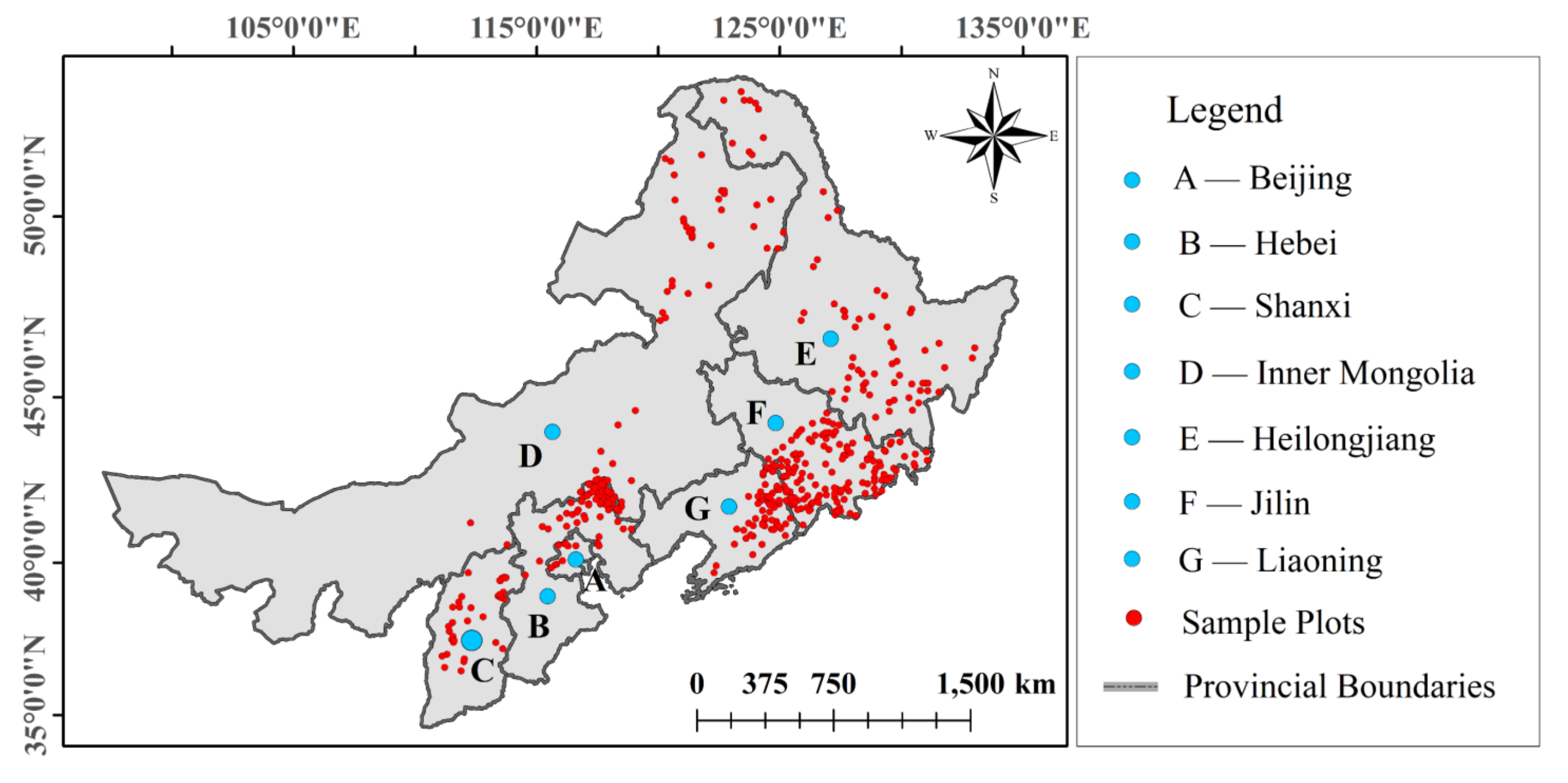
2.1. Sample Plot and Climate Data

The Larix plantation sample plot data were obtained from the 8th (2009–2013) NFI across 7 provinces in northern (Beijing, Hebei, Shanxi, and Inner Mongolia) and northeastern (Heilongjiang, Jilin, and Liaoning) China (Figure 1). Each province represents a population and NFI data were collected over a survey period of 5 years [51,52]. The area of a sample plot was 0.0667 ha in Beijing and Shanxi, 0.08 ha in Liaoning, and 0.06 ha in the remaining provinces. The diameter of a living tree with a diameter at breast height (dbh, 1.3 m) ≥ 5 cm was measured and used to deduce the stand volume (V), quadratic mean diameter (Dg), basal area (Ba), and stem density (N) within each plot. Other measures stand characteristics included stand age and average height (H), with H obtained by measuring 3 to 5 intermediate trees using a Blume–Leiss hypsometer in the sample plot. The allometric models released by the State Forestry Administration of China [53] (Equations (1)–(4) for larch) and Wang [54] (not listed for associated tree species) were used to estimate individual tree aboveground biomass (AGB_tree) and tree total biomass (TB_tree) from dbh, then AGB_tree and TB_tree were summed for all trees and converted to the stand-level aboveground biomass (AGB) and total biomass (TB). Data for sample plots with a total number of trees of less than 20 were eliminated, resulting in 445 valid sample plots.

Table 1. Summary statistics of stand and climate variables across the north and northeast China (n = 445).

Factors	Variables	Units	Mean	Min.	Max.	S.D.	Description
Stand	AGB	t/ha	53.98	2.75	168.07	33.49	Stand aboveground biomass
	TB	t/ha	72.05	3.74	226.50	44.53	Stand total biomass
	H	m	12.0	4.2	24.0	4.0	Stand average height
	Dg	cm	13.4	6.0	26.4	4.3	Stand quadratic mean diameter at breast height
	V	m3/ha	82.81	3.28	282.25	53.22	Stand volume
	Ba	m2/ha	13.55	0.93	38.48	7.63	Stand basal area
	N	trees/ha	1021	263	3933	595	Stand density
	Age	a	28	11	60	9	Stand average age
Climate	AHM	-	22.5	11.7	39.8	4.9	Annual heat-moisture index (MAT + 10)/(MAP/1000))
	CMD	-	185	35	382	74	Hargreaves climate moisture deficit
	DD_0	days	1537	425	3250	513	Degree-days below 0 °C
	DD_18	days	5332	3601	7867	788	Degree-days below 18 °C
	DD18	days	191	12	489	108	Degree-days above 18 °C
	DD5	days	1882	1012	2707	354	Degree-days above 5 °C
	EMT	°C	−30.5	−43.8	−17.7	4.2	Extreme minimum temperature over a 30-year period
	EREF	°C	701	510	912	60	Extreme maximum temperature over a 30-year period
	EXT	-	32.6	25.5	35.1	1.5	Hargreaves reference evaporation
	MAP	mm	625	382	1050	146	Mean annual precipitation
	MAT	°C	3.6	−4.0	9.2	2.4	Mean annual temperature
	MCMT	°C	−16.0	−27.0	−5.6	3.9	Mean coldest month temperature
	MWMT	°C	20.4	14.8	24.0	1.9	Mean warmest month temperature
	NFFD	days	171	111	224	20	The number of frost-free days
	PAS	mm	52	14	133	21	Precipitation as snow between August in previous year and July in current year
	TD	°C	36.4	25.0	45.2	3.8	Temperature difference between MWMT and MCMT, or continentality

showed a statistical summary of stand factors in the present study. The data for the sixteen climate variables (Table 1) were downloaded according to geographical coordinates and elevation of each sample plot using the ClimateAP (v2.11) software (http://ClimateAP.net) (accessed on 15 July 2019). ClimateAP can generate scale-free historical (1901–2015) climate data for specific locations in the Asia Pacific [55]. The present study obtained candidate climate values by averaging from 1981 to 2010.

AGB_tree and TB_tree were derived from dbh according to Equations (1) and (2) for eastern Inner Mongolia, Heilongjiang, Jilin, and Liaoning provinces, and Equations (3 and (4) for central and western Inner Mongolia, Beijing, Hebei, and Shanxi provinces.

AGB_tree = 0.11270dbh^2.39582 (kg),

(1)

TB_tree = 0.11270dbh^2.39582 + 0.042583dbh^2.37053 (kg),

(2)

AGB_tree = 0.07302dbh^2.47298 (kg),

(3)

TB_tree = 0.07302dbh^2.47298 + 0.028287dbh^2.36403 (kg).

(4)

2.2. Random Forests Algorithm

RF is a supervised machine learning algorithm, which combines multiple decision trees together to make a more accurate prediction. We used RF to solve regression problems with the “randomForest” package [56] in R Version 4.0.3. Detailed description on RF algorithm was omitted in the study, but tuning hyper-parameters and quantifying variables importance were key steps when running the model.

Two hyper-parameters are required for optimization in random forests algorithm, namely ntree and mtry, with the former representing the number of regression tree models to develop and the latter representing the number of independent variables randomly sampled as candidates at each split. The default values of ntree and mtry for regression are 500 and int P/3, respectively, where P is the number of independent variables. However, the use of default parameter values does not guarantee an optimal model [57] and optimization of hyper-parameters is recommended to acquire robust predicted results. So, grid search and 10-fold cross-validation was applied for hyper-parameters tuning. Combinations of possible values of ntree and mtry were tested for training and validation data. The optimal hyper-parameter values were determined according to model efficiency and errors.

RF can identify the importance scores of the predictor variables according to the out of the bag error [37]. In a random forests model trained with a set of hyper-parameters, about 36.8% (an average) of the observations in the train data are not used for individual regression tree, that is out of the bag (OOB) data. The importance of the independent variable ($X_j$) was calculated by the mean sum of squares of residuals on OOB data (MSE_OOB) reduction for all regression trees when OOB data for X_j is permuted while all others are left unchanged. The variable importance (VI) score of X_j was attained from Equations (5)–(7) [58].

$${\mathrm{MSE}}_{\mathrm{OOB},t}(X_j)=\frac{1}{n_{\mathrm{OOB},t}}{\displaystyle {\sum }_{i=1}^{n_{{}_{\mathrm{OOB},t}}}{\left[y_{\mathrm{OOB},t,i}-{\widehat{y}}_{\mathrm{OOB},t,i}(X_j)\right]}^2}$$

(5)

$${\mathrm{MSE}}_{\mathrm{OOB},t}({X^{\prime }}_j)=\frac{1}{n_{\mathrm{OOB},t}}{\displaystyle {\sum }_{i=1}^{n_{{}_{\mathrm{OOB},t}}}{\left[y_{\mathrm{OOB},t,i}-{\widehat{y}}_{\mathrm{OOB},t,i}({X^{\prime }}_j)\right]}^2}$$

(6)

$$\mathrm{VI}=\frac{1}{t}{\displaystyle {\sum }_{i=1}^t\left[{\mathrm{MSE}}_{\mathrm{OOB},t}({X^{\prime }}_j{)-\mathrm{MSE}}_{\mathrm{OOB},t}(X_j)\right]}$$

(7)

where, ${\mathrm{MSE}}_{\mathrm{OOB},t}\left(X_j\right)$ and ${\mathrm{MSE}}_{\mathrm{OOB},t}\left({X^{\prime }}_j\right)$ are the mean sum of squares of residuals on OOB data based on $X_j$ and ${X^{\prime }}_j$ ($X_j$ is permuted), respectively; $n_{\mathrm{OOB},t}$ is sample size of OOB data for regression tree t; t is the number of regression tree (the hyper-parameter ntree); $y_{\mathrm{OOB},t,i}$ is the ith observed values of OOB data for regression tree t; and ${\widehat{y}}_{\mathrm{OOB},t,i}(X_j)$ and ${\widehat{y}}_{\mathrm{OOB},t,i}({X^{\prime }}_j)$ are the ith predicted values for regression tree t using OOB data for $X_j$ and ${X^{\prime }}_j$, respectively.

The present study calculated the relative importance of all predictors to quantify their contributions to stand biomass, with the importance values normalized to a percentage as relative importance [43].

2.3. Climate-Sensitive Stand Biomass Model Development

Stand AGB and TB were regarded as separate dependent variables, whereas the considered predictors comprised 22 stand and climate factors (see Table 1 for definitions). Stand factors included Dg, H, Ba, N, V, and stand age, whereas climate variables included AHM, CMD, DD_0, DD_18, DD18, DD5, EMT, EREF, EXT, MAP, MAT, MCMT, MWMT, NFFD, PAS, and TD. The present study tested hyper-parameters by sequences of parameter values (ntree = 50, 100, 150, … 1,500; mtry = 2, 3, … 22). A total of 630 RF models were tested and a 10-fold cross-validation was applied to assess the models and to select the optimal hyper-parameters separately for stand AGB and TB models.

2.4. Model Validation and Evaluation

Three goodness-of-fit statistics were used in the present study for evaluating the performance of the RF models using 10-fold cross-validation, which were the coefficient of determination (R²), root mean square error (RMSE), and relative root mean square error (RRMSE), calculated according to Equations (8)–(10), respectively. Each evaluation indicator was averaged to verify the model performance for the 10 resampled validation datasets. In addition, the optimal values of hyper-parameters ntree and mtry with the smallest RMSE were used to develop the model for the full dataset, after which the model was applied for further analysis.

$$R_{}^2=\frac{1}{k}{\displaystyle \sum _{j=1}^k(1-\frac{{\displaystyle \sum _{i=1}^{n_j}{(B_{{}^{ij}}^{}-{\widehat{B}}_{{}^{ij}}^{})}^2}}{{\displaystyle \sum _{i=1}^{n_j}{(B_{{}^{ij}}^{}-{\overline{B}}_{{}^j}^{})}^2}})}$$

(8)

$$RMSE=\frac{1}{k}{\displaystyle \sum _{j=1}^k(\sqrt{\frac{{\displaystyle \sum _{i=1}^{n_j}{(B_{{}^{ij}}^{}-{\widehat{B}}_{{}^{ij}}^{})}^2}}{n_{{}^j}^{}}})}$$

(9)

$$RRMSE=\frac{1}{k}{\displaystyle \sum _{j=1}^k(\frac{RMS{E}_{{}^j}^{}}{{\overline{B}}_{{}^j}^{}}\times 100\%)}$$

(10)

where k is the number of folds (k = 10 in the present study), $B_{ij}$ and ${\widehat{B}}_{ij}$ represent the ith observed and predicted stand biomass values of the jth folds, respectively, ${\overline{B}}_j$ is the ith observed stand mean biomass of the jth fold, RMSE_j is the root mean square error (RMSE) of the jth fold and n_j is the number of samples of the jth fold.

3. Results

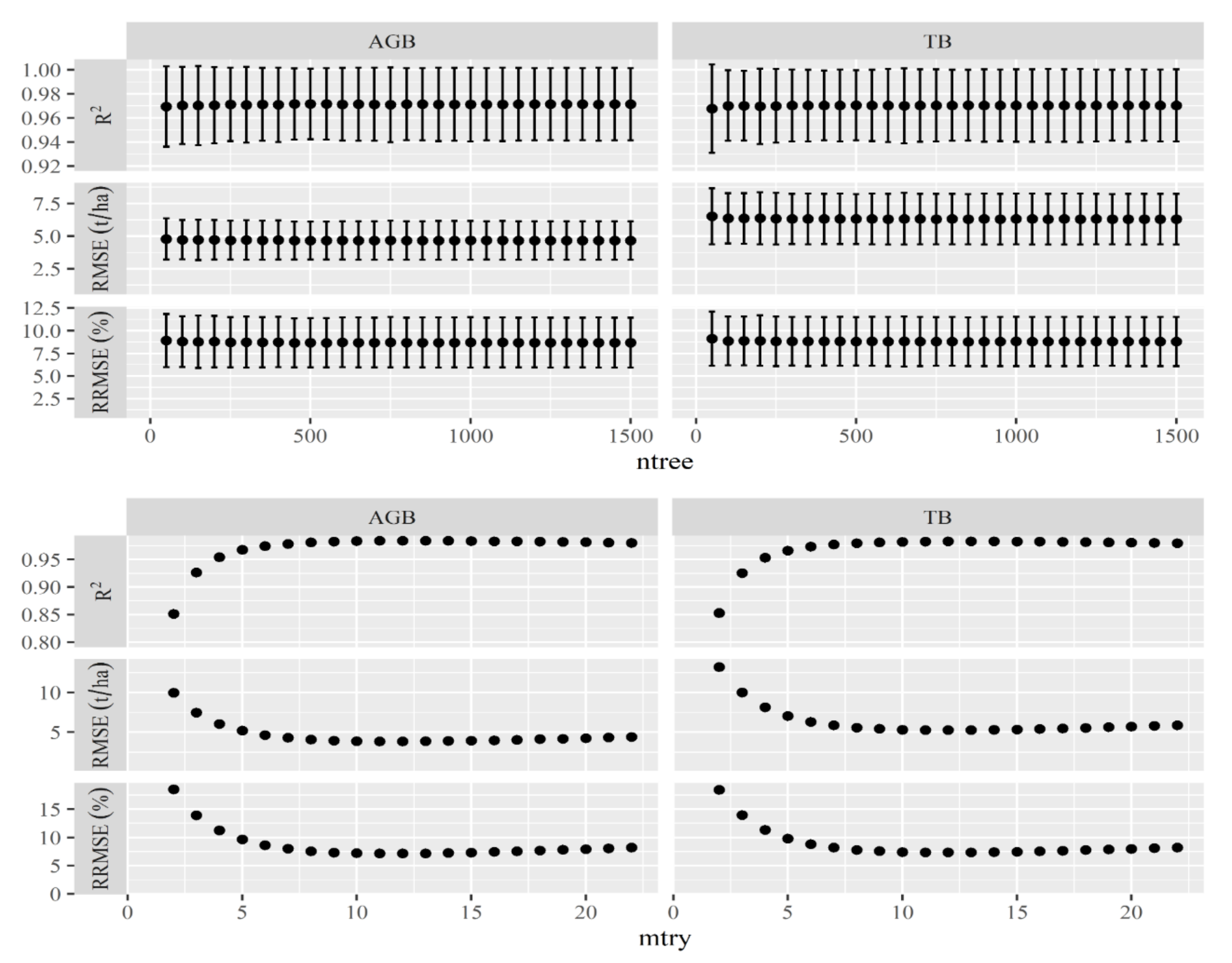
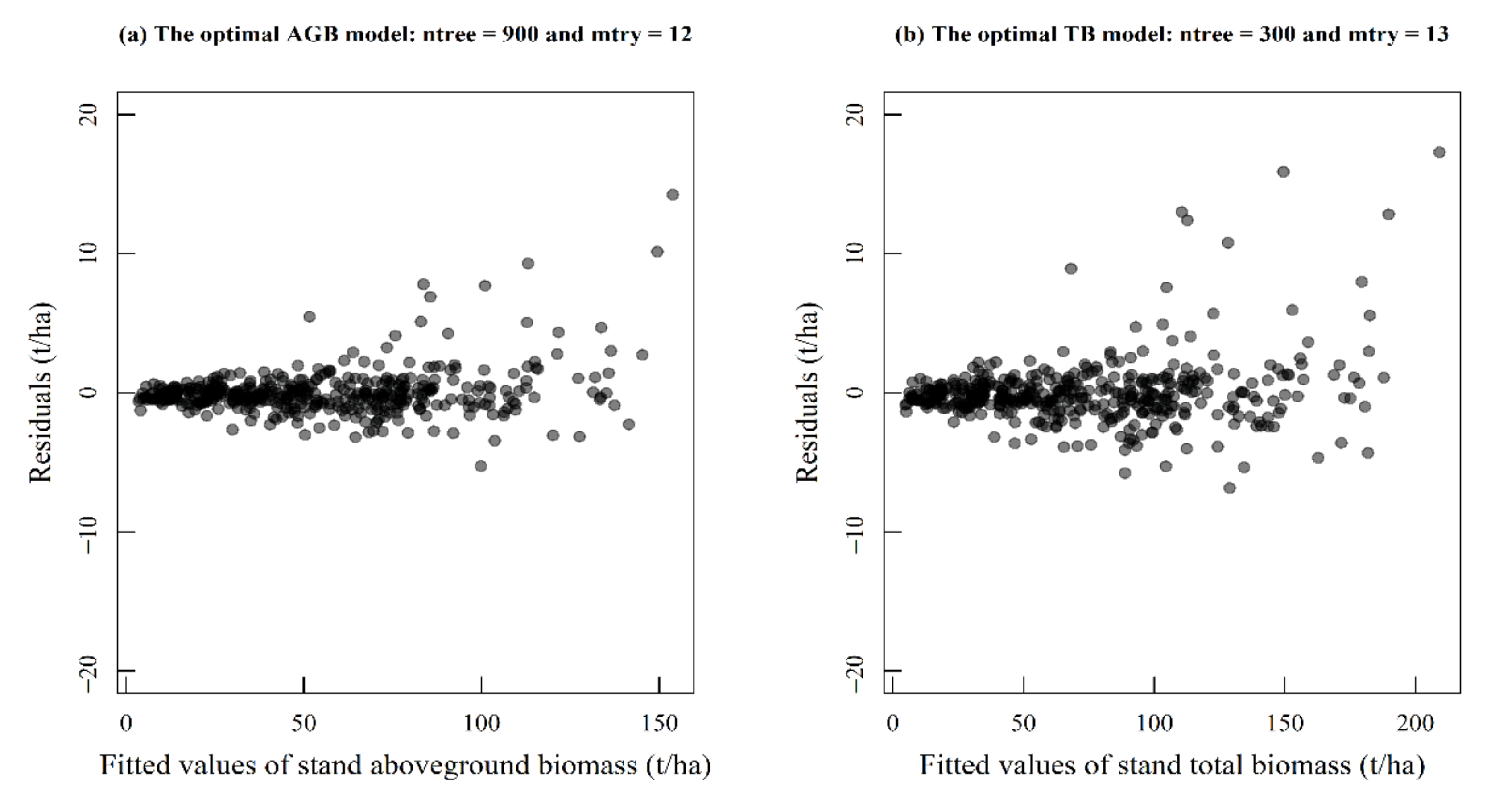
3.1. The Optimal Model

There were large variations in R², RMSE, and RRMSE for different hyper-parameter values (ntree and mtry) of the RF model used to simulate AGB and TB (Figure 2). Generally, with increasing mtry, the R² of the AGB model initially increased and then stabilized at values exceeding 8. In contrast, both RMSE and RRMSE initially decreased, stabilized at values between 8 and 15, and continued an increasing trend at values between 15 and 22. Finally, the minimum RMSE indicated the RF model with ntree = 900 and mtry = 12 to be the optimal climate-sensitive AGB model with R² = 0.9845 ± 0.0095, RMSE = 3.8008 ± 1.135 t ha⁻¹, and RRMSE = 7.0671 ± 2.1095%.

Although similar model performances with different hyper-parameter values were found for the TB model, the optimal values of hyper-parameters were different from those of the AGB model. Specifically, optimal ntree and mtry were 300 and 13, respectively, producing R² = 0.9836 ± 0.0102, RMSE = 5.1963 ± 1.5904 t ha⁻¹, and RRMSE = 7.2418% ± 2.273%.

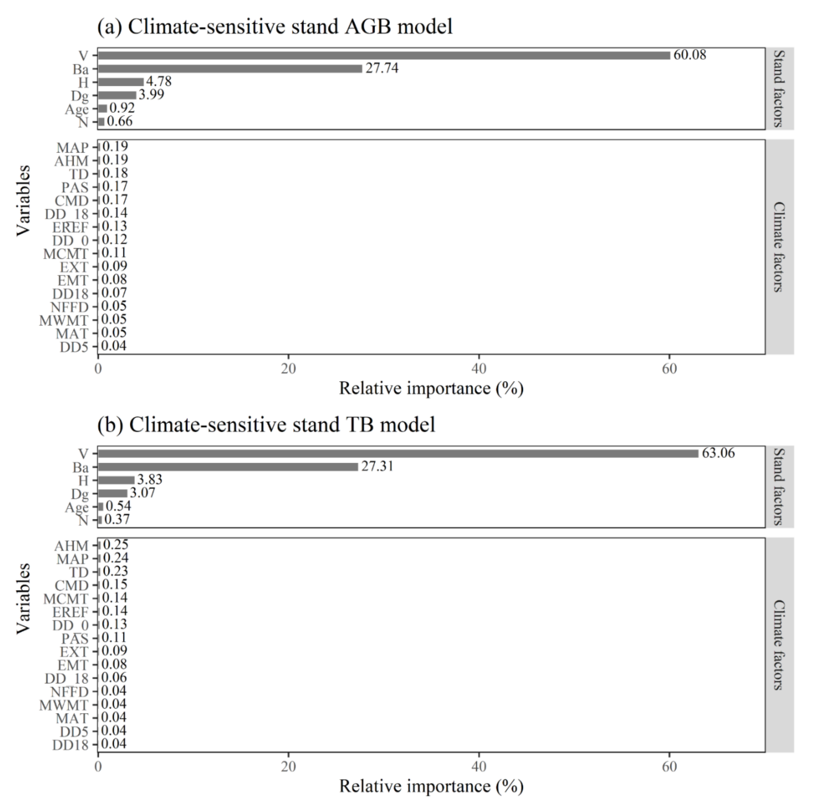
3.2. Relative Importance of Stand and Climate Factors

The relative importance of stand factors in explaining the variation in stand biomass within both the AGB and TB models far exceeded that of climate factors (Figure 3), with stand factors and climate factors having a cumulative relative importance of 98.17% and 1.83%, respectively in the AGB model. The rank of stand factors according to importance was: V > Ba > H > Dg > age > N. The rank of the five most important climate factors was: MAP = AHM > TD > PAS = CMD, with the relative importance of the remaining climate variables ranging between 0.04–0.19%. Similar results were found for the TB model, with relative importance of the AHM, MAP, TD, and CMD variables of 0.25%, 0.24%, 0.23%, and 0.15%, respectively. The cumulative relative importance of stand factors within the TB model was 98.18%, whereas that of climate factors was 1.82%, and no single climate factor had a relative importance exceeding 1%.

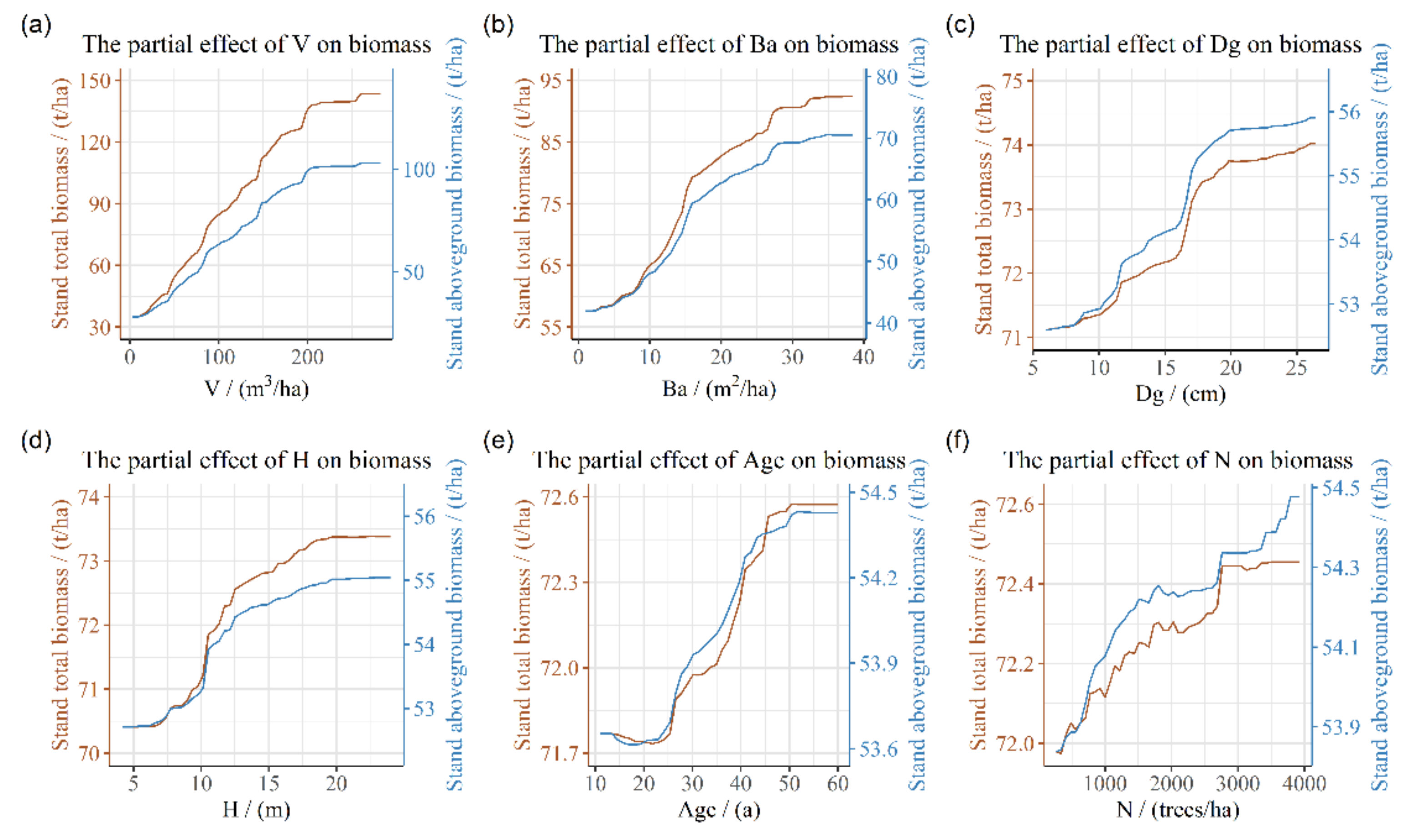
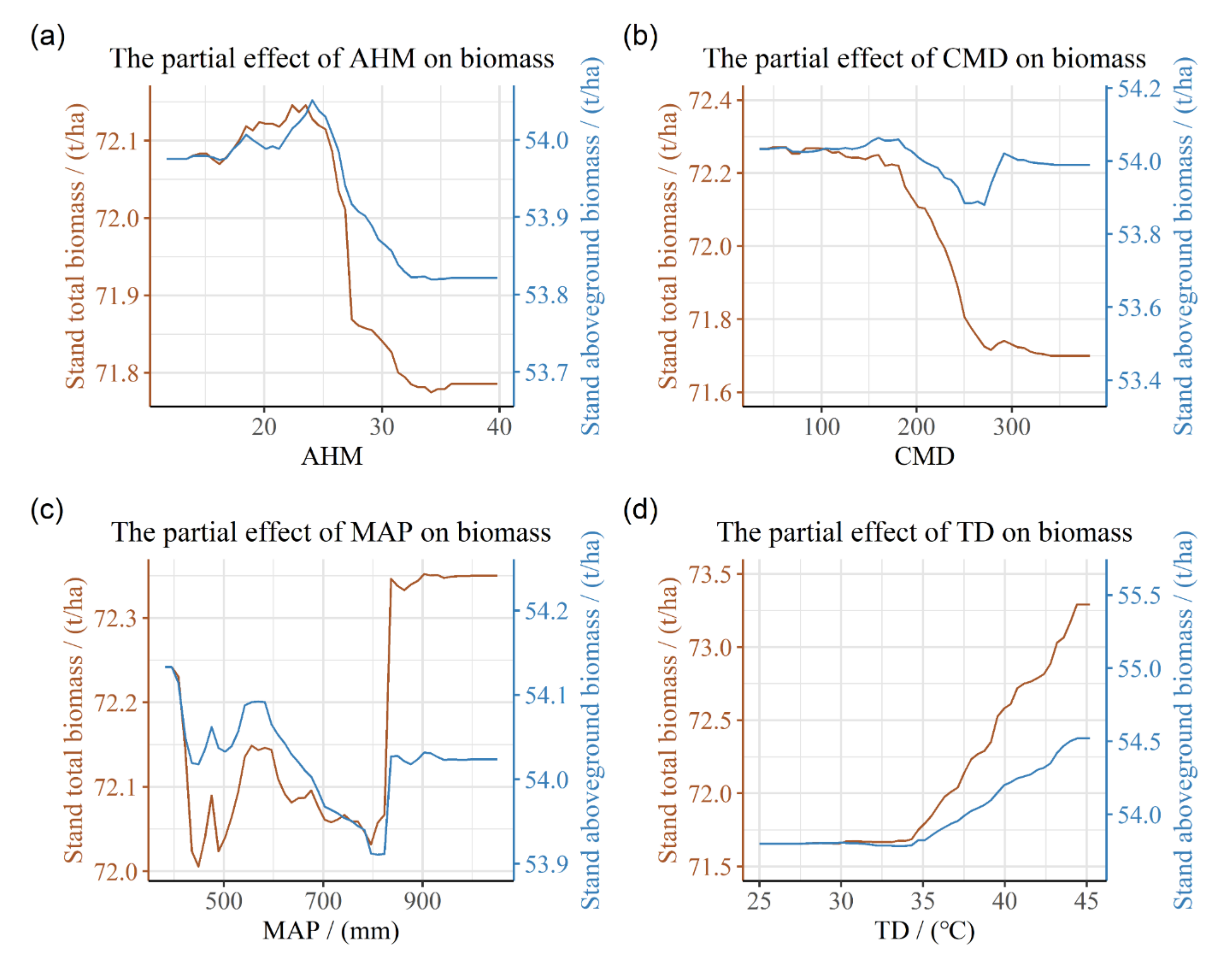
3.3. Partial Dependence of Stand Biomass on Stand and Climate Factors

Stand biomass showed an initial rapid increase and was followed by a gradual increase with increasing stand factors, i.e., V, Ba, Dg, H, and N. The change in AGB and TB with age showed a uniform “S” shape relationship (Figure 4) in which stand biomass showed an initial rapid increase and was followed by stabilization with increasing age. For example, AGB reached a maximum of 54.4 t ha⁻¹ at an age close to 50 a, after which AGB stabilized.

Stand biomass showed a complicated relationship with climate factors. Four important climate variables (AHM, CMD, MAP, and TD) with large relative importance were chosen in the current study to visualize their individual partial effects (Figure 5). The trends of AGB and TB with climate factors were similar. Stand biomass almost did not change with increasing TD up to a threshold of 35 °C, after which stand biomass increased with increasing TD. The relationships of stand biomass with AHM and CMD were opposite to that of TD, with no initial change in stand biomass with increasing AHM and CMD until certain thresholds, after which stand biomass decreased. However, stand biomass showed a fluctuating relationship with MAP.

4. Discussion

4.1. Applications of the Random Forests Algorithm for Estimating Stand Biomass

The present study applied the RF algorithm for developing stand biomass models across large-scale with the inclusions of climate variables. The results showed that the climate-sensitive stand biomass models explained 98.45% and 98.36% of variations in stand AGB and TB, respectively. Therefore, the results illustrated that the RF algorithm could be applied for highly accurate prediction of stand biomass. The higher R² obtained for the AGB model compared to that of the TB model could be attributed to the variability of root biomass.

Traditional regression models for AGB and TB of larch plantations were also developed for comparisons with RF. These models were divided into two categories (independent variables were V, AHM and TD for one group, and BA, H, AHM and TD for the other group) because of collinearity among input variables from RF (

Table 2. Estimated parameters and statistics of traditional regression models.

Model	RMSE (t ha−1)	RRMSE
AGB = 0.2249V0.9558AHM0.1536TD0.2228	5.2501 ± 1.1921	9.8075% ± 2.4826%
AGB = 0.7202BA0.9639H0.4079AHM−0.1341TD0.3287	4.9730 ± 0.6162	9.2079% ± 0.7672%
AGB model based on RF with ntree = 900 and mtry = 12	3.8008 ± 1.1350	7.0671% ± 2.1095%
TB = 0.2117V0.9471AHM0.1056TD0.3718	6.4483 ± 1.5948	9.0377% ± 2.5060%
TB = 0.7295BA0.9420H0.4296AHM−0.1687TD0.4362	6.9059 ± 0.9002	9.5804% ± 0.8853%
TB model based on RF with ntree = 300 and mtry = 13	5.1963 ± 1.5904	7.2418% ± 2.2730%

Note: all parameters in the traditional regression models were significant at 0.05 level. See Table 1 for the definitions of stand and climatic variables.

). Results showed that the traditional regression models had higher errors (RMSE and RRMSE) than RF models. Compared with traditional models, RMSE of RF models decreased by 27.62% for AGB and 19.41% for TB based on V, AHM and TD, respectively; and RMSE of RF models decreased by 23.54% for AGB and 24.78% for TB based on BA, H, AHM and TD, respectively. The RRMSE values of RF models were also lower than those of traditional regression models. Therefore, model performances of the RF in the current study were better than traditional regression models, confirming that RF methods can be applied for estimating stand biomass. Zhang et al. [59] compared the performance of parametric and non-parametric models for predicting aboveground biomass using predictors such as H and N. The results of their study found that the RF model showed a better performance with an R² = 0.9616. Liu et al. [60] developed an AGB model based on RF, with the model achieving a satisfactory performance with an R² = 0.95. RF has some advantages for predicting stand biomass in comparison with traditional regression models. RF is insensitive to collinearity, allowing it to consider multiple variables simultaneously [61]. The structure of the RF algorithm allows easy implementation of parallel processing, thereby improving the speed of computation. The RF model could produce the relative importance of independent variables, and the partial dependence plots for describing nonlinear relationships between the independent variables and dependent variables. In contrast, it is difficult to implement variable selections through the use of traditional regression models when two (or more) independent variables are highly interrelated [62]. The present study illustrated that consideration of both stand and climate factors within the RF model contributed to a high accuracy of biomass prediction. The application of ML (e.g., RF, support vector machines or artificial neural networks) for biomass modelling requires optimization of the hyper-parameters. The widely used parameter tuning methods included grid, random, and Bayesian search [63,64,65,66]. These methods suffer from several disadvantages: the optimal combination of parameters cannot be guaranteed in random search and Bayesian search requires a large number of samples to increase the dimension of the search space. However, grid search identifies the global maximum or minimum when there are few hyper-parameter combinations to be optimized, which is very robust. The present study adopted grid search, which is usually applied to data with spatial and/or temporal structure [67]. As illustrated in the present study, although default values of hyper-parameters are used in practice, the use of optimal hyper-parameters allowed more accurate estimation of stand biomass (Figure 2). However, a persisting disadvantage of the RF approach was the residual heteroscedasticity of the biomass model (Figure 6), resulting in underestimation of stand biomass, particularly for larger predicted values. Future studies should aim to address this issue.

4.2. Relationship between Stand Factors and Stand Biomass

Stand variables such as V, Ba, H, N, the stand density index (SDI), Dg, and age are often used as key predictors within a stand biomass model [4,8,20,24,47,68]. The present study showed that the cumulative relative importance of stand factors for predicting stand biomass was close to 98% (Figure 4). Among the predictors, V was the most important, with a relative importance of over 60%. This result also confirmed the validity of the volume-derived biomass method widely applied based on the relationships between volume and biomass at the stand or forest level [3,69]. The results are supported by previous studies which showed that stand biomass or carbon had strong positive correlations with Ba [70,71] and H [72,73]. In fact, the combination of Ba and H is equivalent to stand volume, thereby strengthening the biomass–volume relationship. The present study also considered the important S-shaped relationship between age and stand biomass (Figure 4), which is in accordance with the general growth pattern of trees. However, age showed a weaker relationship with stand biomass compared with V and other stand factors. This can be attributed to V being a function of stand growth and therefore having a direct effect on stand biomass. In contrast, age is a one-dimensional variable which mainly has an indirect effect on stand biomass [74]. In addition, the stand biomass of larch plantations increased with increasing N, which was consistent with the findings of previous studies [68,75]. Biodiversity and stand structure are also important drivers of stand biomass [76,77]. However, the present study did not consider biodiversity due to the monoculture nature of Larix plantations. Future studies can examine stand structure effects.

4.3. Relationship between Climate Factors and Stand Biomass

Forest biomass varied with climate, showing natural spatial variation closely related to drought, temperature, or precipitation [78]. However, the influence of climate factors on stand biomass in the present study was relatively weak compared with that of stand variables, with a cumulative relative importance of only 2%. This does not mean that the effect of climate on stand biomass should be ignored. He et al. [21] found that not considering climate variables resulted in large differences in estimated forest carbon sequestration at large scales. In addition, previous studies reported that the inclusion of climate variables improved model performances at the individual tree or stand level [12,13,19,20,21]. However, these models considered different climate variables, including MAT (°C), long-term average growing season temperature (°C), January MAT (°C), mean temperature of wettest quarter (°C), MAP (mm), total growing season precipitation (mm), precipitation of the driest quarter and precipitation of the wettest quarter (mm) [12,13,19,20,23,79,80,81]. The present study found that the four most important climate variables for explaining stand biomass were AHM, CMD, MAP, and TD. AHM and CMD can reflect the humidity of a forest area, which is important for estimating both AGB and TB. An increase in AHM can lead to excessive temperature or increased evaporation, resulting in an increase in CMD, which limits the water absorption efficiency of vegetation [82]. This in turn hinders photosynthesis and ultimately leads to a decline in biomass (Figure 5). Correspondingly, a rising temperature in wet areas can result in an increase in stand biomass, whereas an opposite pattern occurs in dry areas [83]. On the other hand, under situations of temperature determining productivity in cold zones, forests will adapt to an excessively low temperature of the mean coldest month by greatly increasing photosynthesis and accumulating greater quantities of energy during the growing-season [84]. Therefore, temperature and precipitation usually simultaneously influence stand biomass. Furthermore, the relationship between climate variables and biomass was inconsistent. Luo et al. [80] proposed that there were no significant correlations between stand biomass and MAP for Pinus yunnanensis, whereas a significant negative correlation existed between MAT and stand biomass. However, Wang et al. [85] showed that stand biomass increased linearly with increasing precipitation. This inconsistency may be due to species-specific sensitivity to climate. The warming and precipitation-induced increase in tree productivity may be a direct effect of either increased photosynthesis or an indirect effect resulting from increased rates of litter decomposition. These effects led to an increase in the accumulation of biomass, which was more obvious in arid areas [86]. Hence, the impact of climate change on stand biomass varies among different tree species and regions, and it is undeniable that climate variables have an important impact on forest biomass and should be included in biomass models.

4.4. Uncertainty Analysis on Stand Biomass Estimation

When using regression model to predict forest biomass at large scale, the sources of uncertainty of estimated results included [87,88,89,90,91]: (1) measurement error of forest area [92,93]; (2) measurement error of independent variables [94,95]; and (3) the model error [94,95,96]. Relevant studies showed that biomass model error was the main source of uncertainty in biomass estimation [94]. In this study, we found that the stand biomass model without climate variables (ntree = 950 and mtry = 3 for AGB, and ntree = 300 and mtry = 3 for TB) established by using the same method had higher uncertainty than climate-sensitive stand biomass models, and RMSE of climate-sensitive stand biomass models decreased by 5.13% for AGB and 11.52% for TB, respectively. Therefore, using climate variables as independent variables is an effective way to reduce biomass model uncertainty [79]. Furthermore, although the climate variables only had less than 2% contribution to stand biomass, the estimation error would be large when scaling up from sample plot to large scale regions using stand biomass models without climate variables, which was approved by our previous study [21]. In addition, our study did not consider the seedling biomass with trees’ dbh less than 5 cm because of the data limitations. According to the protocol of NFI in China, only trees with dbh larger than 5cm were recorded. In the literature of large-scale forest biomass estimation using NFI data, the minimum dbh was generally 5 cm [97,98,99]. Meanwhile, there are many examples of forests biomass assessment using NFI data with trees’ dbh ≥5cm, such as Puliti et al. [33] and Hauglin et al. [34]. However, the biomass of small trees also played an important role in the global carbon cycle and soil preservation [100,101,102,103,104]. Stegen et al. [18] reported that the trees dbh less than 10 cm and lianas could represent over 10% of a forest’s biomass [105]. Therefore, the seedling biomass should be included for accurate forest biomass estimates in future study.

5. Conclusions

The present study developed climate-sensitive stand aboveground and total biomass models for larch plantations in northern and northeastern China based on the RF algorithm. The aboveground biomass and total biomass models showed good performances with R² values of 0.9845 and 0.9836, respectively. Among the input variables, the cumulative relative importance values of stand and climate factors in explaining stand biomass were >98% and <2%, respectively. The partial dependences of stand biomass on climate and stand variables were consistent with current understanding of the factors affecting tree growth. These results will help increase the accuracy of forests biomass modeling and support decision-making in forest carbon sequestration management. Therefore, RF is a potential effective method for estimating stand biomass. The climate-sensitive forest biomass models developed in this study are useful tools for assessing forest carbon sequestration services under climate change and large-scale carbon stock mapping.

References

1. Pan, Y.; Birdsey, R.A.; Fang, J.; Houghton, R.; Kauppi, P.E.; Kurz, W.A.; Phillips, O.L.; Shvidenko, A.; Lewis, S.L.; Canadell, J.G. A large and persistent carbon sink in the world’s forests. Science 2011, 333, 988–993. [Google Scholar] [CrossRef] [PubMed] [Green Version]
2. De Groot, R.S.; Alkemade, R.; Braat, L.; Hein, L.; Willemen, L. Challenges in integrating the concept of ecosystem services and values in landscape planning, management and decision making. Ecol. Complex. 2010, 7, 260–272. [Google Scholar] [CrossRef]
3. Fang, J.; Chen, A.; Peng, C.; Zhao, S.; Ci, L. Changes in forest biomass carbon storage in China between 1949 and 1998. Science 2001, 292, 2320–2322. [Google Scholar] [CrossRef] [PubMed]
4. Bi, H.; Long, Y.; Turner, J.; Lei, Y.; Snowdon, P.; Li, Y.; Harper, R.; Zerihun, A.; Ximenes, F. Additive prediction of aboveground biomass for Pinus radiata (D. Don) plantations. For. Ecol. Manag. 2010, 259, 2301–2314. [Google Scholar] [CrossRef]
5. Jagodziński, A.M.; Dyderski, M.K.; Gęsikiewicz, K.; Horodecki, P. Tree-and stand-level biomass estimation in a Larix decidua Mill. Chronosequence. Forests 2018, 9, 587. [Google Scholar] [CrossRef] [Green Version]
6. Jagodziński, A.M.; Dyderski, M.K.; Gęsikiewicz, K.; Horodecki, P. Tree and stand level estimations of Abies alba Mill. aboveground biomass. Ann. For. Sci. 2019, 76, 56. [Google Scholar] [CrossRef] [Green Version]
7. Hu, M.; Lehtonen, A.; Minunno, F.; Mäkelä, A. Age effect on tree structure and biomass allocation in Scots pine (Pinus sylvestris L.) and Norway spruce (Picea abies [L.] Karst.). Ann. For. Sci. 2020, 77, 90. [Google Scholar] [CrossRef]
8. Dong, L.; Zhang, L.; Li, F. Evaluation of stand biomass estimation methods for major forest types in the eastern Da Xing’an Mountains, Northeast China. Forests 2019, 10, 715. [Google Scholar] [CrossRef] [Green Version]
9. Miettinen, J.; Ollikainen, M.; Nieminen, T.M.; Ukonmaanaho, L.; Laurén, A.; Hynynen, J.; Lehtonen, M.; Valsta, L. Whole-tree harvesting with stump removal versus stem-only harvesting in peatlands when water quality, biodiversity conservation and climate change mitigation matter. For. Policy Econ. 2014, 47, 25–35. [Google Scholar] [CrossRef]
10. Bessaad, A.; Bilger, I.; Korboulewsky, N. Assessing Biomass Removal and Woody Debris in Whole-Tree Harvesting System: Are the Recommended Levels of Residues Ensured? Forests 2021, 12, 807. [Google Scholar] [CrossRef]
11. Suchomel, C.; Pyttel, P.; Becker, G.; Bauhus, J. Biomass equations for sessile oak (Quercus petraea (Matt.) Liebl.) and hornbeam (Carpinus betulus L.) in aged coppiced forests in southwest Germany. Biomass Bioenergy 2012, 46, 722–730. [Google Scholar] [CrossRef]
12. Fu, L.; Lei, X.; Hu, Z.; Zeng, W.; Tang, S.; Marshall, P.; Cao, L.; Song, X.; Yu, L.; Liang, J. Integrating regional climate change into allometric equations for estimating tree aboveground biomass of Masson pine in China. Ann. For. Sci. 2017, 74, 42. [Google Scholar] [CrossRef] [Green Version]
13. Zeng, W.; Duo, H.; Lei, X.; Chen, X.; Wang, X.; Pu, Y.; Zou, W. Individual tree biomass equations and growth models sensitive to climate variables for Larix spp. in China. Eur. J. For. Res. 2017, 136, 233–249. [Google Scholar] [CrossRef]
14. Cysneiros, V.C.; de Souza, F.C.; Gaui, T.D.; Pelissari, A.L.; Orso, G.A.; do Amaral Machado, S.; de Carvalho, D.C.; Silveira-Filho, T.B. Integrating climate, soil and stand structure into allometric models: An approach of site-effects on tree allometry in Atlantic Forest. Ecol. Indic. 2021, 127, 107794. [Google Scholar] [CrossRef]
15. Rohner, B.; Waldner, P.; Lischke, H.; Ferretti, M.; Thürig, E. Predicting individual-tree growth of central European tree species as a function of site, stand, management, nutrient, and climate effects. Eur. J. For. Res. 2018, 137, 29–44. [Google Scholar] [CrossRef]
16. Chave, J.; Réjou-Méchain, M.; Búrquez, A.; Chidumayo, E.; Colgan, M.S.; Delitti, W.B.; Duque, A.; Eid, T.; Fearnside, P.M.; Goodman, R.C. Improved allometric models to estimate the aboveground biomass of tropical trees. Glob. Change Biol. 2014, 20, 3177–3190. [Google Scholar] [CrossRef]
17. Schaphoff, S.; Reyer, C.P.; Schepaschenko, D.; Gerten, D.; Shvidenko, A. Tamm Review: Observed and projected climate change impacts on Russia’s forests and its carbon balance. For. Ecol. Manag. 2016, 361, 432–444. [Google Scholar] [CrossRef] [Green Version]
18. Stegen, J.C.; Swenson, N.G.; Enquist, B.J.; White, E.P.; Phillips, O.L.; Jørgensen, P.M.; Weiser, M.D.; Monteagudo Mendoza, A.; Núñez Vargas, P. Variation in above-ground forest biomass across broad climatic gradients. Glob. Ecol. Biogeogr. 2011, 20, 744–754. [Google Scholar] [CrossRef]
19. Usoltsev, V.A.; Shobairi, S.O.R.; Tsepordey, I.S.; Chasovskikh, V.P. Modeling the additive structure of stand biomass equations in climatic gradients of Eurasia. Environ. Qual. Manag. 2018, 28, 55–61. [Google Scholar] [CrossRef]
20. Usoltsev, V.; Kovyazin, V.; Tsepordey, I.; Chasovskikh, V. What is a possible response of forest biomass to changes in Eurasian air temperature and precipitation? A special case for the genus Betula spp. In Proceedings of the IOP Conference Series: Earth and Environmental Science, Saint Petersburg, Russian Federation, 16–18 June 2020; p. 012084. [Google Scholar]
21. He, X.; Lei, X.-D.; Dong, L.-H. How large is the difference in large-scale forest biomass estimations based on new climate-modified stand biomass models? Ecol. Indic. 2021, 126, 107569. [Google Scholar] [CrossRef]
22. Keith, H.; Mackey, B.G.; Lindenmayer, D.B. Re-evaluation of forest biomass carbon stocks and lessons from the world’s most carbon-dense forests. Proc. Natl. Acad. Sci. USA 2009, 106, 11635–11640. [Google Scholar] [CrossRef] [PubMed] [Green Version]
23. Raich, J.W.; Russell, A.E.; Kitayama, K.; Parton, W.J.; Vitousek, P.M. Temperature influences carbon accumulation in moist tropical forests. Ecology 2006, 87, 76–87. [Google Scholar] [CrossRef] [PubMed] [Green Version]
24. Lei, X.; Zhang, H.; Mou, H. Compatible stand biomass models of Mongolia oak forests in over logged forest regions, Northeast China. Quat. Sci. 2010, 30, 559–565, (In Chinese with English Abstract). [Google Scholar]
25. Ashraf, M.I.; Zhao, Z.; Bourque, C.P.-A.; MacLean, D.A.; Meng, F.-R. Integrating biophysical controls in forest growth and yield predictions with artificial intelligence technology. Can. J. For. Res. 2013, 43, 1162–1171. [Google Scholar] [CrossRef]
26. Hamidi, S.K.; Zenner, E.K.; Bayat, M.; Fallah, A. Analysis of plot-level volume increment models developed from machine learning methods applied to an uneven-aged mixed forest. Ann. For. Sci. 2021, 78, 4. [Google Scholar] [CrossRef]
27. Yousafzai, A.; Manzoor, W.; Raza, G.; Mahmood, T.; Rehman, F.; Hadi, R.; Shah, S.; Amin, M.; Akhtar, A.; Bashir, S. Forest yield prediction under different climate change scenarios using data intelligent models in Pakistan. Braz. J. Biol. 2021, 84. Available online: https://www.scielo.br/j/bjb/a/vBgTRjcxmgyFZR3TFqRVr8r/?lang=en (accessed on 1 March 2022). [CrossRef]
28. Görgens, E.B.; Montaghi, A.; Rodriguez, L.C.E. A performance comparison of machine learning methods to estimate the fast-growing forest plantation yield based on laser scanning metrics. Comput. Electron. Agric. 2015, 116, 221–227. [Google Scholar] [CrossRef]
29. Jachowski, N.R.; Quak, M.S.; Friess, D.A.; Duangnamon, D.; Webb, E.L.; Ziegler, A.D. Mangrove biomass estimation in Southwest Thailand using machine learning. Appl. Geogr. 2013, 45, 311–321. [Google Scholar] [CrossRef]
30. Zhang, J.; Huang, S.; Hogg, E.; Lieffers, V.; Qin, Y.; He, F. Estimating spatial variation in Alberta forest biomass from a combination of forest inventory and remote sensing data. Biogeosciences 2014, 11, 2793–2808. [Google Scholar] [CrossRef] [Green Version]
31. Gao, Y.; Lu, D.; Li, G.; Wang, G.; Chen, Q.; Liu, L.; Li, D. Comparative analysis of modeling algorithms for forest aboveground biomass estimation in a subtropical region. Remote Sens. 2018, 10, 627. [Google Scholar] [CrossRef] [Green Version]
32. Luo, M.; Wang, Y.; Xie, Y.; Zhou, L.; Qiao, J.; Qiu, S.; Sun, Y. Combination of Feature Selection and CatBoost for Prediction: The First Application to the Estimation of Aboveground Biomass. Forests 2021, 12, 216. [Google Scholar] [CrossRef]
33. Puliti, S.; Hauglin, M.; Breidenbach, J.; Montesano, P.; Neigh, C.; Rahlf, J.; Solberg, S.; Klingenberg, T.; Astrup, R. Modelling above-ground biomass stock over Norway using national forest inventory data with ArcticDEM and Sentinel-2 data. Remote Sens. Environ. 2020, 236, 111501. [Google Scholar] [CrossRef]
34. Hauglin, M.; Rahlf, J.; Schumacher, J.; Astrup, R.; Breidenbach, J. Large scale mapping of forest attributes using heterogeneous sets of airborne laser scanning and National Forest Inventory data. For. Ecosyst. 2021, 8, 65. [Google Scholar] [CrossRef]
35. Vahedi, A.A. Artificial neural network application in comparison with modeling allometric equations for predicting above-ground biomass in the Hyrcanian mixed-beech forests of Iran. Biomass Bioenergy 2016, 88, 66–76. [Google Scholar] [CrossRef]
36. Wu, C.; Chen, Y.; Peng, C.; Li, Z.; Hong, X. Modeling and estimating aboveground biomass of Dacrydium pierrei in China using machine learning with climate change. J. Environ. Manag. 2019, 234, 167–179. [Google Scholar] [CrossRef]
37. Breiman, L. Random forests. Mach. Learn. 2001, 45, 5–32. [Google Scholar] [CrossRef] [Green Version]
38. Breiman, L. Statistical modeling: The two cultures (with comments and a rejoinder by the author). Stat. Sci. 2001, 16, 199–231. [Google Scholar] [CrossRef]
39. Calle, M.L.; Urrea, V. Stability of Random Forest importance measures. Brief. Bioinform. 2011, 12, 86–89. [Google Scholar] [CrossRef] [Green Version]
40. Li, R.; Zhao, S.; Zhao, H.; Xu, M.; Zhang, L.; Wen, H.; Sheng, Q. Spatiotemporal Assessment of Forest Biomass Carbon Sinks: The Relative Roles of Forest Expansion and Growth in Sichuan Province, China. J. Environ. Qual. 2017, 46, 64–71. [Google Scholar] [CrossRef]
41. Kindermann, G.E. The development of a simple basal area increment model. Nat. Preced. 2011, 127, 147–178. [Google Scholar] [CrossRef] [Green Version]
42. Diamantopoulou, M.J.; Özçelik, R.; Yavuz, H. Tree-bark volume prediction via machine learning: A case study based on black alder’s tree-bark production. Comput. Electron. Agric. 2018, 151, 431–440. [Google Scholar] [CrossRef]
43. Ou, Q.; Lei, X.; Shen, C. Individual tree diameter growth models of larch–spruce–fir mixed forests based on machine learning algorithms. Forests 2019, 10, 187. [Google Scholar] [CrossRef] [Green Version]
44. Jevšenak, J.; Skudnik, M. A random forest model for basal area increment predictions from national forest inventory data. For. Ecol. Manag. 2021, 479, 118601. [Google Scholar] [CrossRef]
45. State Forestry and Grassland Administration of China. Report of Forest Resources in China (2014–2018); China Forestry Publishing House: Beijing, China, 2019. [Google Scholar]
46. Zhou, G.; Wang, Y.; Jiang, Y.; Yang, Z. Estimating biomass and net primary production from forest inventory data: A case study of China’s Larix forests. For. Ecol. Manag. 2002, 169, 149–157. [Google Scholar] [CrossRef]
47. Dong, L.; Li, F. Additive stand-level biomass models for natural larch forest in the East of Daxing’ an Mountains. Sci. Silvae Sin. 2016, 52, 13–21, (In Chinese with English Abstract). [Google Scholar]
48. Zang, H.; Lei, X.; Zeng, W. Height–diameter equations for larch plantations in northern and northeastern China: A comparison of the mixed-effects, quantile regression and generalized additive models. For. Int. J. For. Res. 2016, 89, 434–445. [Google Scholar] [CrossRef]
49. Lei, X.; Yu, L.; Hong, L. Climate-sensitive integrated stand growth model (CS-ISGM) of Changbai larch (Larix olgensis) plantations. For. Ecol. Manag. 2016, 376, 265–275. [Google Scholar] [CrossRef]
50. Xie, Y.; Wang, H.; Lei, X. Application of the 3-PG model to predict growth of Larix olgensis plantations in northeastern China. For. Ecol. Manag. 2017, 406, 208–218. [Google Scholar] [CrossRef]
51. Lei, X.; Tang, M.; Lu, Y.; Hong, L.; Tian, D. Forest inventory in China: Status and challenges. Int. For. Rev. 2009, 11, 52–63. [Google Scholar] [CrossRef]
52. Zeng, W.; Tomppo, E.; Healey, S.P.; Gadow, K.V. The national forest inventory in China: History-results-international context. For. Ecosyst. 2015, 2, 23. [Google Scholar] [CrossRef] [Green Version]
53. State Forestry Administration of China. Tree Biomass Models and Related Parameters to Carbon Accounting for Larix; Standards Press of China: Beijing, China, 2016. [Google Scholar]
54. Wang, C. Biomass allometric equations for 10 co-occurring tree species in Chinese temperate forests. For. Ecol. Manag. 2006, 222, 9–16. [Google Scholar] [CrossRef]
55. Wang, T.; Wang, G.; Innes, J.L.; Seely, B.; Chen, B. ClimateAP: An application for dynamic local downscaling of historical and future climate data in Asia Pacific. Front. Agric. Sci. Eng. 2017, 4, 448–458. [Google Scholar] [CrossRef] [Green Version]
56. Liaw, A.; Wiener, M. Classification and regression by randomForest. R News 2002, 2, 18–22. [Google Scholar]
57. Kuhn, M.; Johnson, K. Applied Predictive Modeling; Springer: New York, NY, USA, 2013. [Google Scholar]
58. Grömping, U. Variable importance assessment in regression: Linear regression versus random forest. Am. Stat. 2009, 63, 308–319. [Google Scholar] [CrossRef]
59. Zhang, G.; Yue, C.; Zhao, X.; Luo, H.; Gu, L. Aboveground Biomass Estimation of Simao pinewith Stand Average Height and Density of Plantation. J. Northeast For. Univ. 2021, 49, 16–22, (In Chinese with English Abstract). [Google Scholar]
60. Liu, K.; Wang, J.; Zeng, W.; Song, J. Comparison and evaluation of three methods for estimating forest above ground biomass using TM and GLAS data. Remote Sens. 2017, 9, 341. [Google Scholar] [CrossRef] [Green Version]
61. Cutler, D.R.; Edwards, T.C., Jr.; Beard, K.H.; Cutler, A.; Hess, K.T.; Gibson, J.; Lawler, J.J. Random forests for classification in ecology. Ecology 2007, 88, 2783–2792. [Google Scholar] [CrossRef]
62. Fukuda, S.; Yasunaga, E.; Nagle, M.; Yuge, K.; Sardsud, V.; Spreer, W.; Müller, J. Modelling the relationship between peel colour and the quality of fresh mango fruit using Random Forests. J. Food Eng. 2014, 131, 7–17. [Google Scholar] [CrossRef]
63. Bergstra, J.; Bengio, Y. Random search for hyper-parameter optimization. J. Mach. Learn. Res. 2012, 13, 281–305. [Google Scholar]
64. Xia, Y.; Liu, C.; Li, Y.; Liu, N. A boosted decision tree approach using Bayesian hyper-parameter optimization for credit scoring. Expert Syst. Appl. 2017, 78, 225–241. [Google Scholar] [CrossRef]
65. Fayed, H.A.; Atiya, A.F. Speed up grid-search for parameter selection of support vector machines. Appl. Soft Comput. 2019, 80, 202–210. [Google Scholar] [CrossRef]
66. Sun, Y.; Ding, S.; Zhang, Z.; Jia, W. An improved grid search algorithm to optimize SVR for prediction. Soft Comput. 2021, 25, 5633–5644. [Google Scholar] [CrossRef]
67. Roberts, D.R.; Bahn, V.; Ciuti, S.; Boyce, M.S.; Elith, J.; Guillera-Arroita, G.; Hauenstein, S.; Lahoz-Monfort, J.J.; Schröder, B.; Thuiller, W. Cross-validation strategies for data with temporal, spatial, hierarchical, or phylogenetic structure. Ecography 2017, 40, 913–929. [Google Scholar] [CrossRef]
68. Usoltsev, V.A.; Shobairi, S.O.R.; Tsepordey, I.S.; Chasovkikh, V.P. Modelling forest stand biomass and net primary production with the focus on additive models sensitive to climate variables for two-needled Pines in Eurasia. J. Clim. Change 2019, 5, 41–49. [Google Scholar] [CrossRef]
69. Castedo-Dorado, F.; Gómez-García, E.; Diéguez-Aranda, U.; Barrio-Anta, M.; Crecente-Campo, F. Aboveground stand-level biomass estimation: A comparison of two methods for major forest species in northwest Spain. Ann. For. Sci. 2012, 69, 735–746. [Google Scholar] [CrossRef]
70. Cannell, M. Woody biomass of forest stands. For. Ecol. Manag. 1984, 8, 299–312. [Google Scholar] [CrossRef]
71. Rahman, M.M.; Kabir, M.E.; Akon, A.J.U.; Ando, K. High carbon stocks in roadside plantations under participatory management in Bangladesh. Glob. Ecol. Conserv. 2015, 3, 412–423. [Google Scholar] [CrossRef] [Green Version]
72. Khan, M.N.I.; Shil, M.C.; Azad, M.S.; Sadath, M.N.; Feroz, S.; Mollick, A.S. Allometric relationships of stem volume and stand level carbon stocks at varying stand density in Swietenia macrophylla King plantations, Bangladesh. For. Ecol. Manag. 2018, 430, 639–648. [Google Scholar] [CrossRef]
73. Khan, M.N.I.; Islam, M.R.; Rahman, A.; Azad, M.S.; Mollick, A.S.; Kamruzzaman, M.; Sadath, M.N.; Feroz, S.; Rakkibu, M.G.; Knohl, A. Allometric relationships of stand level carbon stocks to basal area, tree height and wood density of nine tree species in Bangladesh. Glob. Ecol. Conserv. 2020, 22, e01025. [Google Scholar] [CrossRef]
74. Yuan, Z.; Ali, A.; Jucker, T.; Ruiz-Benito, P.; Wang, S.; Jiang, L.; Wang, X.; Lin, F.; Ye, J.; Hao, Z.; et al. Multiple abiotic and biotic pathways shape biomass demographic processes in temperate forests. Ecology 2019, 100, e02650. [Google Scholar] [CrossRef] [Green Version]
75. Xu, Q.; Lei, X.; Guo, H.; Li, H.; Li, Y. Stand biomass model of Larix olgensis plantations based on multi-layer perceptron networks. J. Beijing For. Univ. 2019, 42, 97–107, (In Chinese with English Abstract). [Google Scholar]
76. Ali, A.; Lin, S.-L.; He, J.-K.; Kong, F.-M.; Yu, J.-H.; Jiang, H.-S. Climate and soils determine aboveground biomass indirectly via species diversity and stand structural complexity in tropical forests. For. Ecol. Manag. 2019, 432, 823–831. [Google Scholar] [CrossRef]
77. Gao, W.-Q.; Lei, X.-D.; Liang, M.-W.; Larjavaara, M.; Li, Y.-T.; Gao, D.-L.; Zhang, H.-R. Biodiversity increased both productivity and its spatial stability in temperate forests in northeastern China. Sci. Total Environ. 2021, 780, 146674. [Google Scholar] [CrossRef] [PubMed]
78. Rudgers, J.A.; Hallmark, A.; Baker, S.R.; Baur, L.; Hall, K.M.; Litvak, M.E.; Muldavin, E.H.; Pockman, W.T.; Whitney, K.D. Sensitivity of dryland plant allometry to climate. Funct. Ecol. 2019, 33, 2290–2303. [Google Scholar] [CrossRef]
79. Luo, Y.; Wang, X.; Zhang, X.; Ren, Y.; Poorter, H. Variation in biomass expansion factors for China’s forests in relation to forest type, climate, and stand development. Ann. For. Sci. 2013, 70, 589–599. [Google Scholar] [CrossRef] [Green Version]
80. Luo, H.; Zhang, C.; Wei, A. The Effect of Climate on the Biomass of Pinus yunnanensis Standing Forest. J. Southwest For. Univ. 2017, 37, 99–104, (In Chinese with English Abstract). [Google Scholar]
81. Saatchi, S.S.; HOUGHTON, R.A.; Dos Santos Alvala, R.; Soares, J.V.; Yu, Y. Distribution of aboveground live biomass in the Amazon basin. Glob. Change Biol. 2007, 13, 816–837. [Google Scholar] [CrossRef]
82. Ciais, P.; Reichstein, M.; Viovy, N.; Granier, A.; Ogée, J.; Allard, V.; Aubinet, M.; Buchmann, N.; Bernhofer, C.; Carrara, A. Europe-wide reduction in primary productivity caused by the heat and drought in 2003. Nature 2005, 437, 529–533. [Google Scholar] [CrossRef]
83. Usoltsev, V.A.; Shobairi, S.O.R.; Petrovich, V. Modeling the additive stand biomass of Larix spp. for Eurasia. Ecol. Quest. 2019, 30, 35–46. [Google Scholar]
84. Zhou, G.; Liu, Q.; Xu, Z.; Du, W.; Yu, J.; Meng, S.; Zhou, H.; Qin, L.; Shah, S. How can the shade intolerant Korean pine survive under dense deciduous canopy? For. Ecol. Manag. 2020, 457, 117735. [Google Scholar] [CrossRef]
85. Wang, G.; Guan, D.; Xiao, L.; Peart, M. Forest biomass-carbon variation affected by the climatic and topographic factors in Pearl River Delta, South China. J. Environ. Manag. 2019, 232, 781–788. [Google Scholar] [CrossRef] [PubMed]
86. Becknell, J.M.; Kucek, L.K.; Powers, J.S. Aboveground biomass in mature and secondary seasonally dry tropical forests: A literature review and global synthesis. For. Ecol. Manag. 2012, 276, 88–95. [Google Scholar] [CrossRef]
87. Sileshi, G.W. A critical review of forest biomass estimation models, common mistakes and corrective measures. For. Ecol. Manag. 2014, 329, 237–254. [Google Scholar] [CrossRef]
88. Fu, Y.; Lei, Y.; Zeng, W.; Hao, R.; Zhang, G.; Zhong, Q.; Xu, M. Uncertainty assessment in aboveground biomass estimation at the regional scale using a new method considering both sampling error and model error. Can. J. For. Res. 2017, 47, 1095–1103. [Google Scholar] [CrossRef] [Green Version]
89. Lehtonen, A.; Cienciala, E.; Tatarinov, F.; Mäkipää, R. Uncertainty estimation of biomass expansion factors for Norway spruce in the Czech Republic. Ann. For. Sci. 2007, 64, 133–140. [Google Scholar] [CrossRef] [Green Version]
90. Zhou, X.; Lei, X.; Liu, C.; Huang, H.; Zhou, C.; Peng, C. Re-estimating the changes and ranges of forest biomass carbon in China during the past 40 years. For. Ecosyst. 2019, 6, 51. [Google Scholar] [CrossRef] [Green Version]
91. Wang, Y.; Yue, T.; Lei, Y.; Du, Z.; Zhao, M. Uncertainty of forest biomass carbon patterns simulation on provincial scale: A case study in Jiangxi Province, China. J. Geogr. Sci. 2016, 26, 568–584. [Google Scholar] [CrossRef] [Green Version]
92. Garnett, M.H.; Ineson, P.; Stevenson, A.C.; Howard, D.C. Terrestrial organic carbon storage in a British moorland. Glob. Change Biol. 2001, 7, 375–388. [Google Scholar] [CrossRef] [Green Version]
93. Abella, S.R.; Gering, L.R.; Shelburne, V.B. Slope correction of plot dimensions for vegetation sampling in mountainous terrain. Nat. Areas J. 2004, 24, 358–360. [Google Scholar]
94. Chave, J.; Condit, R.; Aguilar, S.; Hernandez, A.; Lao, S.; Perez, R. Error propagation and scaling for tropical forest biomass estimates. Philos. Trans. R. Soc. London. Ser. B Biol. Sci. 2004, 359, 409–420. [Google Scholar] [CrossRef]
95. Liu, C.; Zhou, X.; Lei, X.; Huang, H.; Zhou, C.; Peng, C.; Wang, X. Separating Regressions for model fitting to reduce the uncertainty in forest volume-biomass relationship. Forests 2019, 10, 658. [Google Scholar] [CrossRef] [Green Version]
96. Keller, M.; Palace, M.; Hurtt, G. Biomass estimation in the Tapajos National Forest, Brazil: Examination of sampling and allometric uncertainties. For. Ecol. Manag. 2001, 154, 371–382. [Google Scholar] [CrossRef]
97. Poorter, L.; Bongers, F.; Aide, T.M.; Almeyda Zambrano, A.M.; Balvanera, P.; Becknell, J.M.; Boukili, V.; Brancalion, P.H.; Broadbent, E.N.; Chazdon, R.L. Biomass resilience of Neotropical secondary forests. Nature 2016, 530, 211–214. [Google Scholar] [CrossRef] [PubMed]
98. Anderson-Teixeira, K.J.; Davies, S.J.; Bennett, A.C.; Gonzalez-Akre, E.B.; Muller-Landau, H.C.; Joseph Wright, S.; Abu Salim, K.; Almeyda Zambrano, A.M.; Alonso, A.; Baltzer, J.L. CTFS-Forest GEO: A worldwide network monitoring forests in an era of global change. Glob. Change Biol. 2015, 21, 528–549. [Google Scholar] [CrossRef] [PubMed] [Green Version]
99. Rozendaal, D.M.; Suarez, D.R.; De Sy, V.; Avitabile, V.; Carter, S.; Yao, C.A.; Alvarez-Davila, E.; Anderson-Teixeira, K.; Araujo-Murakami, A.; Arroyo, L. Aboveground forest biomass varies across continents, ecological zones and successional stages: Refined IPCC default values for tropical and subtropical forests. Environ. Res. Lett. 2022, 17, 014047. [Google Scholar] [CrossRef]
100. Bloomberg, M.; Mason, E.G.; Jarvis, P.; Sedcole, R. Predicting seedling biomass of radiata pine from allometric variables. New For. 2008, 36, 103–114. [Google Scholar] [CrossRef]
101. Panda, M.R.; Oraon, P.R.; Tirkey, P. Distribution of woody biomass reserves in tropical dry Sal (Shorea robusta roth.) forests of Ranchi. Pharma Innov. J. 2020, 9, 477–482. [Google Scholar]
102. Kaarakka, L.; Tamminen, P.; Saarsalmi, A.; Kukkola, M.; Helmisaari, H.-S.; Burton, A.J. Effects of repeated whole-tree harvesting on soil properties and tree growth in a Norway spruce (Picea abies (L.) Karst.) stand. For. Ecol. Manag. 2014, 313, 180–187. [Google Scholar] [CrossRef]
103. Aherne, J.; Posch, M.; Forsius, M.; Lehtonen, A.; Härkönen, K. Impacts of forest biomass removal on soil nutrient status under climate change: A catchment-based modelling study for Finland. Biogeochemistry 2012, 107, 471–488. [Google Scholar] [CrossRef]
104. Augusto, L.; Achat, D.L.; Bakker, M.R.; Bernier, F.; Bert, D.; Danjon, F.; Khlifa, R.; Meredieu, C.; Trichet, P. Biomass and nutrients in tree root systems–sustainable harvesting of an intensively managed Pinus pinaster (Ait.) planted forest. Gcb Bioenergy 2015, 7, 231–243. [Google Scholar] [CrossRef]
105. Chave, J.; Condit, R.; Lao, S.; Caspersen, J.P.; Foster, R.B.; Hubbell, S.P. Spatial and temporal variation of biomass in a tropical forest: Results from a large census plot in Panama. J. Ecol. 2003, 91, 240–252. [Google Scholar] [CrossRef]
Figure 1. Map of sample plots of larch plantations across the north and northeast China.
Sustainability 14 05580 g001
Figure 2. Performance of the climate-sensitive stand biomass model with different values of the ntree and mtry parameters in random forests according to 10-fold cross validation. AGB and TB stand for aboveground biomass and total biomass, respectively.
Sustainability 14 05580 g002
Figure 3. Relative importance score of each independent variable in the stand biomass model. (a)—the climate sensitive aboveground biomass (AGB) model, (b)—the climate-sensitive total biomass (TB) model.
Sustainability 14 05580 g003
Figure 4. Partial dependence plots illustrating the relationships between stand biomass and V (a), Ba (b), Dg (c), H (d), age (e), and N (f). See Table 1 for the definitions of stand variables.
Sustainability 14 05580 g004
Figure 5. Partial dependence plots illustrating the relationships between stand biomass and AHM (a), CMD (b), MAP (c), and TD (d). See Table 1 for the definitions of climate variables.
Sustainability 14 05580 g005
Figure 6. Distributions of residuals for the optimal models (a) climate-sensitive stand aboveground biomass model, (b) climate-sensitive stand total biomass model.
Sustainability 14 05580 g006