Hybrid Predictive Modeling for Charging Demand Prediction of Electric Vehicles

Abstract

In recent years, the supply of electric vehicles, which are eco-friendly cars that use electric energy rather than fossil fuels, which cause air pollution, is increasing. Accordingly, it is emerging as an urgent task to predict the charging demand for the smooth supply of electric energy required to charge electric vehicle batteries. In this paper, to predict the charging demand, time series analysis is performed based on two types of frames: One is using traditional time series techniques such as dynamic harmonic regression, seasonal and trend decomposition using Loess, and Bayesian structural time series. The other is the most widely used machine learning techniques, including random forest and extreme gradient boosting. However, the tree-based machine learning approaches have the disadvantage of not being able to capture the trend, so a hybrid strategy is proposed to overcome this problem. In addition, the seasonal variation is reflected as the feature by using the Fourier transform which is useful in the case of describing the seasonality patterns of time series data with multiple seasonality. The considered time series models are compared and evaluated through various accuracy measures. The experimental results show that the machine learning approach based on the hybrid strategy generally achieves significant improvements in predicting the charging demand. Moreover, when compared with the original machine learning method, the prediction based on the proposed hybrid strategy is more accurate than that based on the original machine learning method. Based on these results, it can find out that the proposed hybrid strategy is useful for smoothly planning future power supply and demand and efficiently managing electricity grids.

1. Introduction

The World Health Organization (WHO) cited air pollution and climate change as the biggest factors that harm human health in a report titled “Ten threats to global health in 2019”. The WHO also said 9 out of 10 people breathe polluted air every day, which could cause 7 million premature deaths each year. Fine dust is the most harmful air pollutant to the human body. Fine dust can reduce cognitive function, increase the probability of dementia, cause heart and respiratory diseases, and may reduce vision. In addition, fine dust destroys the ecosystem by acidifying soil and water with acid rain and affects semiconductors and industrial activities. As fine dust has an adverse effect in various areas, efforts are needed to reduce it. In particular, countries around the world are regulating emissions of internal combustion locomotives and introducing eco-friendly cars to reduce automobile emissions, which are the main cause of fine dust. A representative type of eco-friendly car is the electric vehicle (EV). Unlike existing internal combustion engines that use gasoline or light oil, EVs use electric energy through batteries as a power source, so harmful emissions such as carbon dioxide or nitrogen oxides are not emitted. For this reason, EVs are recognized as a symbol of eco-friendly cars around the world, and global automakers are focusing their efforts on developing eco-friendly EVs. As a result, global EV sales are estimated to be 3.24 million units in 2020, up about 43% year-on-year according to EV Volumes, which is a global EV market research company. In particular, Korea, which was reported as the country with the worst air pollution among the Organization for Economic Co-operation and Development member countries through the “2019 World Air Quality Report”, is encouraging the purchase of EVs through subsidies and tax benefits to reduce automobile emissions.

However, EVs still have many problems, including the cost of purchase, short mileage due to battery limitations, long charging time, location of charging stations, and lack of public charging infrastructure. In particular, the lack of charging infrastructure is the biggest obstacle to the growth of the EV market. The way to resolve this problem is to increase the number of fast-charging stations, but it is impossible to install many fast chargers due to expensive installation costs. Therefore, to reduce the inconvenience of EV users, charging stations should be installed in the optimal location, and some studies [1,2,3,4,5] have suggested ways to select the appropriate charging station location.

Another issue with EVs is the charging demand (CD). Sales of EVs are growing exponentially, so the CD will also increase. The future CD must be able to accommodate the expanding supply of EVs, and it is important to accurately predict the amount of electricity for charging to establish a smooth supply and demand plan [6]. Furthermore, predicting the CD helps to efficiently manage electrical grids [7]. Realizing the importance of this CD, some researchers have applied various models to predict the CD. Majidpour et al. [8] studied forecasting of the CD of EVs from the customer profile data and station records data using support vector regression (SVR) and random forest (RF). Choi et al. [6] predicted the CD by region using EV charging stations data in Seoul and Jeju Island based on the autoregressive integrated moving average (ARIMA), ARIMA with an exogenous variable, ARIMA generalized autoregressive conditionally heteroskedastic models, and so on. They considered various features including the number of EVs registered and holidays. Almaghrebi et al. [7] applied the machine learning (ML) techniques such as RF, extreme gradient boosting (XGBoost), and support vector machine to predict the CD of plug-in EVs. They used weekday, season, the time of day when the EV plugs in, and so on, as the feature. Lee et al. [9] devised an imputation method on how to handle missing values in EV charging data and provided a long-short-term-memory (LSTM)-based forecasting model of EV charging station load. Kim and Kim [10] analyzed the CD of EVs in Korea through the artificial neural network and LSTM, considering the temperature, weekends, and holidays as the feature. Chang et al. [11] suggested a framework for predicting fast-CD based on deep learning approaches and techniques, including a continuous sliding window and weight initialization. Lan et al. [12] proposed the ML approach based on SVR and the modified dragonfly algorithm to predict the CD of hybrid EVs. In addition, several studies have attempted to predict the CD of EVs without applying ML methods. Lopez et al. [13] proposed a new approach to model the CD of EVs based on discrete event simulation. Liu et al. [14] proposed a fast CD prediction model based on the intelligent sensing system of dynamic EVs under EVs–traffic-distribution coupling. Yi et al. [15] developed the modified geographical PageRank model to estimate the CD of EVs.

However, the tree-based ML techniques such as RF and XGBoost logically make rules and predict future values only by rules made by training data, so it is impossible to predict higher values than the maximum values found in the training data. Likewise, a value lower than the minimum value found in the training data also cannot be predicted. This in turn makes the trend unable to be captured. Despite this limitation, the classical studies for the prediction of the CD do not consider the decomposition of time series data in applying the tree-based ML techniques. This paper overcomes the limitation by providing a hybrid strategy that combines the trend component captured from the traditional time series technique with the detrended component analyzed by the ML techniques. In addition, unlike the classical studies, the Fourier terms are used as features to take into account the seasonal factors associated with cycles because it is very useful in describing the seasonality patterns of time series data with multiple seasonality. To implement the proposed method, data on the CD of EVs in Korea are used for analysis. The amount of data to be used for training is not large enough to perform a deep learning (DL) technique, so this paper focuses on comparing the ML techniques and traditional time series methods. For the traditional time series analysis, dynamic harmonic regression (DHR), STLM, and Bayesian structural time series (BSTS) are used. RF and XGBoost are used as the ML techniques to which the hybrid strategy will be applied.

The remainder of the paper is structured as follows. Section 2 introduces the time series methods to be used in the analysis to predict the CD. Section 3 describes features considered with exploring the data and shows the process and results of data analysis. Finally, Section 4 concludes.

2. Models for Hybrid Strategy

As mentioned earlier, the hybrid strategy is proposed to analyze the decomposed time series data because the tree-based ML techniques cannot capture the trend. Moreover, the Fourier terms are considered as features to handle the seasonality of time series data.

To capture the trend component of the time series data, the most commonly used ARIMA model for predicting non-stationary time series with the trend or seasonality is applied. The ARIMA model includes three factors: an autoregression (AR) term, a moving average (MA) term, and a difference and is given by

$$\begin{array}{c}\hfill \left(1-{\varphi }_{1}B-\dots -{\varphi }_p{B}^p\right){\left(1-B\right)}^d{Y}_t=\left(1+{\theta }_{1}B+\dots +{\theta }_q{B}^q\right){ϵ}_t,{ϵ}_t\sim WN(0,{\sigma }_{ϵ}^2),\end{array}$$

where p and q denote the orders of the AR and MA terms, respectively, and d denotes the number of differences required to make a stationary time series. The back-shift operator B denotes $B{Y}_t=Y_{t-1}$.

The Fourier term reflecting the seasonal variation is given by

$$\begin{array}{c}\hfill {\left(sin\left({\omega }_{i}t\right),cos\left({\omega }_{i}t\right)\right)}_{i=1}^K,\end{array}$$

where ${\omega }_i$ is defined as $2\pi i/m$ with a seasonal period m and $K(\le m/2)$ is the number of sine and cosine pairs.

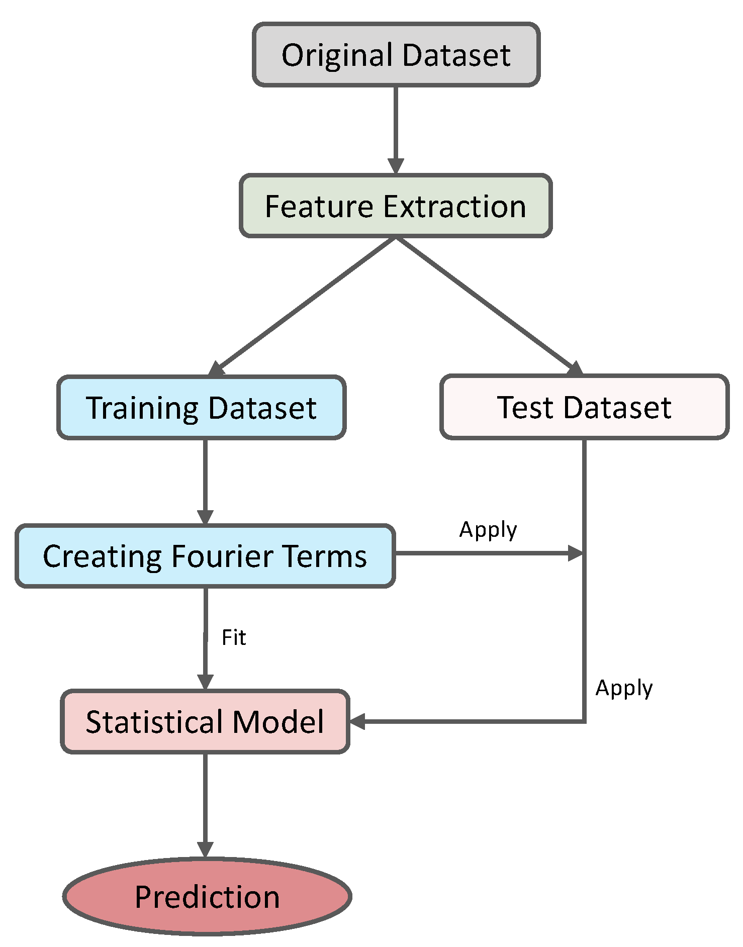
The overall prediction frameworks based on the statistical and ML models are illustrated as schematic diagrams in Figure 1 and Figure 2.

The models considered for the CD analysis are described sequentially in the following subsection.

2.1. Statistical Model

As the statistical model, the two frequentist models and one Bayesian model are considered. In the frequentist approach, the DHR and the seasonal and trend decomposition using Loess (STL) model are used for the CD modeling.

First, the DHR is a regression model with the Fourier terms which can approximate any periodic function as a sum of sine and cosine functions. In particular, the DHR is useful in time series data with a long seasonal period such as hourly time series data which is often observed due to the development of technology. The DHR with a regression component is given by

$$\begin{array}{c}\hfill Y_t={\beta }_0+\sum _{i=1}^j{\beta }_{i,t}{x}_{i,t}+\sum _{i=1}^K\left[{\alpha }_{i,t}sin\left({\omega }_{i}t\right)+{\gamma }_{i,t}cos\left({\omega }_{i}t\right)\right]+{\eta }_t,\end{array}$$

where $Y_t$ is the observed time series data at time t, ${\beta }_{i,t}$ is the coefficient for the ith covariate $x_{i,t}$ at time t, ${\alpha }_{i,t}$ and ${\gamma }_{i,t}$ are unobserved stochastic time variable parameters, and ${\eta }_t$ is modeled as a non-seasonal ARIMA process for handling the short-term dynamics. This model has the advantage of being able to allow any length of seasonality, including Fourier terms of different frequencies for time series data with multiple seasonal periods [16].

Another frequentist approach, STL, is known not only to be a versatile and robust method for decomposing time series, but also to be able to deal with any type of seasonality including monthly and quarterly data [16]. Assuming that the STL performs an additive decomposition of a time series, the time series data $Y_t$ is decomposed given by

$$\begin{array}{c}\hfill Y_t=A_t+S_t.\end{array}$$

Here, the seasonally adjusted component $A_t$, which represents the sum of the trend and remainder components, can be modeled and predicted by some time series analysis method. The seasonal component $S_t$ is forecasted using the seasonal naïve method. Then, the final prediction value is obtained by adding the predicted value of the seasonal component $S_t$ to the predicted value of the seasonally adjusted component $A_t$.

The BSTS model is a model in which the Bayesian framework is applied to the structural time series (STS) model, which is the state-space model for time series data. By denoting $Y_t$ as the observed time series data and ${\alpha }_t$ as the system state at time t, the STS model consists of two equations: one is the observation equation:

$$\begin{array}{cc}\hfill Y_t& =Z_t^T{\alpha }_t+{ϵ}_t,\hfill \end{array}$$

(1)

where $Z_t$ is an output matrix and the error term ${ϵ}_t$ has a normal distribution with mean $\mu =0$ and variance ${\sigma }^2=H_t$; the other is the state/transition equation:

$$\begin{array}{cc}\hfill {\alpha }_{t+1}& =T_t{\alpha }_t+R_t{\eta }_t,t\ge 1,\hfill \end{array}$$

(2)

where $T_t$ and $R_t$ are transition and control matrices, respectively, and the error term ${\eta }_t$ has a normal distribution with mean $\mu =0$ and variance ${\sigma }^2=Q_t$. The matrices $Z_t$, $T_t$, and $R_t$ typically contain unknown parameters and known values, which are often set as 0 and 1. In addition, ${ϵ}_t$ and ${\eta }_t$ are generally assumed to be serially uncorrelated and also to be uncorrelated with each other at all time periods. Thanks to the flexibility and modularity of the model, it can express a very large class of models including all ARIMA models [17]. For example, in Equations (1) and (2), the following local level model can be obtained by setting all of $Z_t$, $T_t$, and $R_t$ to 1 and substituting ${\alpha }_t$ with ${\mu }_t$:

$$\begin{array}{cc}\hfill & Y_t={\mu }_t+{ϵ}_t,\hfill \\ \hfill & {\mu }_{t+1}={\mu }_t+{\eta }_t.\hfill \end{array}$$

A useful model adding a regression component ${\mathit{\beta }}^{\mathit{T}}{\mathit{x}}_{\mathit{t}}$ to the basic structure of the BSTS model written by Durbin and Koopman [18] is given by

$$\begin{array}{cc}\hfill Y_t& ={\mu }_t+{\tau }_t+{\mathit{\beta }}^{\mathit{T}}{\mathit{x}}_{\mathit{t}}+{ϵ}_t,{ϵ}_t\sim N(0,{\sigma }_{ϵ}^2),\hfill \\ \hfill {\mu }_{t+1}& ={\mu }_t+{\delta }_t+u_t,u_t\sim N(0,{\sigma }_u^2),\hfill \\ \hfill {\delta }_{t+1}& ={\delta }_t+v_t,v_t\sim N(0,{\sigma }_v^2),\hfill \\ \hfill {\tau }_{t+1}& =-\sum _{s=1}^{S-1}{\tau }_{t+1-s}+w_t,w_t\sim N(0,{\sigma }_w^2),\hfill \end{array}$$

where ${\mu }_t$ and ${\delta }_t$ are the level and slope of the trend at time t, respectively. ${\tau }_t$ is the seasonal component, which can be thought of as a set of S dummy variables with dynamic coefficients constrained to have zero expectation over a full cycle of S seasons. For the variance parameter ${\sigma }_{ϵ}^2$ and the regression coefficient $\beta$, a spike and slab prior [19] is applied and the prior of other variance parameters ${\sigma }_u^2,{\sigma }_v^2,{\sigma }_w^2$ is assumed to be a gamma prior which is a conjugate prior distribution.

2.2. Machine Learning Techniques

The ensemble technique prevents overfitting and enables more accurate prediction than individual models by combining multiple models to create one powerful model. Depending on the learning method, it can be largely divided into bagging, boosting, and stacking. A brief description of ML techniques representing each of these three approaches is provided.

RF [20] is an ML technique widely used for classification and regression because it exhibits strong performance. It utilizes a bagging technique, which is an abbreviation for bootstrap aggregating, where the bootstrap means to generate a dataset of the same size as the original training dataset by allowing duplicates in the given training data and randomly sampling. The RF generates many decision trees using the dataset generated by the bootstrap technique, and the final prediction is made by collecting the results of each individual decision tree. The final prediction is determined by a majority vote (classification) or average value (regression) from the prediction of many decision trees generated. Moreover, the most notable point of RF is to find the best feature among randomly selected candidate features instead of looking for the best feature among the entire feature when splitting nodes in the tree, which can prevent overfitting. This randomness makes learning easy and fast and increases the prediction accuracy by creating decorrelated decision trees.

The XGBoost is an improved ML technique in terms of the speed and performance of the gradient boosting algorithm implemented using a boosting technique to learn multiple weak learners sequentially. The boosting learns the next model by reflecting the errors of the previous model, so it is slower to create the model than bagging, but has fewer errors. The gradient boosting algorithm, a representative boosting algorithm, builds a tree-based model using gradient descent to reduce the loss. However, it has the disadvantages of quickly occurring the overfitting, and requiring a long time because it is not parallelized. To overcome these shortcomings, Chen and Guestrin [21] introduced XGBoost, which is an optimized distributed gradient boosting library designed to be highly efficient, flexible, and portable. XGBoost has the advantages of being fast in learning with parallelism and being able to perform well in classification and regression. In addition, it prevents overfitting and enables early termination.

Note that RF and XGBoost have the hyperparameters that must be set in advance to perform learning. These hyperparameters can control the complexity of the model and play an important role in determining the predictive power of the model. The description of the hyperparameters for each ML technique is given in

Table 1. Description of the hyperparameters for the ML techniques.

	Hyperparameter	Description
RF	mtry	Number of features randomly selected as candidates at each split
	ntree	Number of trees to grow
	nodesize	Minimum size of terminal nodes
XGBoost	nrounds	Number of boosting iterations
	eta	Learning rate
	max_depth	Maximum depth of a tree
	gamma	Minimum loss reduction required to make a split
	min_chile_weight	Minimum sum of the instance weight needed in a child
	subsample	Subsample ratio of training data
	colsample_bytree	Ratio for subsampling of features

.

Stacking is similar to bagging and boosting in that it combines several individual algorithms to produce predictive results. However, the biggest difference is that it uses the prediction results generated by individual algorithms as the input data for the final model. This study considers XGBoost and a generalized linear model (GLM) as a final model for combining multiple individual algorithms. In particular, by using GLM as the final model, it can be expected to make a robust linear combination for predictions of individual models.

3. Analysis

A dataset (http://keco.or.kr/, accessed on 10 August 2020) on the operation status of EV charging stations recorded from 1 January 2014 to 14 September 2017 that was acquired from Korea Environment Corporation is used for analysis. The data that collected the CD of fast chargers installed nationwide consist of the name of the charging station, region, charging start time, charging end time, CD, and so on. To extract features, an exploratory analysis first is conducted, given in the following subsection.

3.1. Feature Extraction

For a more accurate prediction, it is necessary to consider several features that can affect the CD.

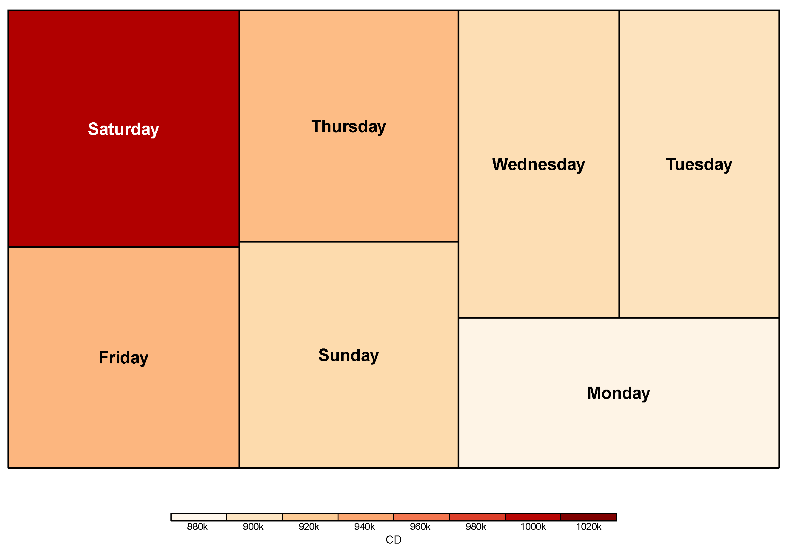
In general, the traffic is expected to be heavy on holidays and weekends, which means holidays and weekends can affect predicting the CD. To confirm this, the CD according to the days of the week is shown in Figure 3. Note that the darker the color, the higher the CD is. Contrary to the expectation that weekends will be higher, Figure 3 shows that Thursday and Friday have higher CDs than Sunday. Based on Figure 3, we consider the feature that represents 1 if the days of the week charging an EV is Thursday, Friday, or Saturday, and 0 otherwise.

The hour is considered as another feature. Figure 4 shows the CD according to the hour, which indicates that the CD is the highest from 3 P.M. to 5 P.M. (15 h to 17 h). Meanwhile, the CD is less from 12 to 6 in the morning than in the afternoon.

Figure 5 represents the CD according to the hour and the days of the week as the three-dimensional scatter plot. The CD according to the hour has a similar pattern for all days of the week, which can be expected to show daily seasonality.

To address the seasonality, the seasonal variables generated by the Fourier transform are considered as features, unlike conventional studies. Based on Figure 5, the hourly data may be assumed daily seasonality with a seasonal period of 24. Additionally, to handle weekly seasonality, the hourly data are assumed weekly seasonality with a seasonal period of 168. Then, the following Fourier terms using $K=2$ can be generated for the dataset:

$$\begin{array}{c}\hfill {\left(sin\left(\frac{2\pi it}{24}\right),cos\left(\frac{2\pi it}{24}\right)\right)}_{i=1}^2,{\left(sin\left(\frac{2\pi it}{168}\right),cos\left(\frac{2\pi it}{168}\right)\right)}_{i=1}^2.\end{array}$$

Finally, public holidays and quarter are considered as the feature.

Table 2. Features of interest for predicting the CD from the CD data.

Feature	Type	Description
Hour	Numeric	Hour of day when the EV charges
Quarter	Categorical	1 = January to March, 2 = April to June, 3 = July to September, 4 = October to December
Weekday	Categorical	Thursday, Friday, Saturday (1 = Yes, 0 = No)
Holiday	Categorical	Public holidays (1 = Yes, 0 = No)
S1-24	Numeric	Fourier daily term $\left(sin\left(2\pi t/24\right)\right)$
C1-24	Numeric	Fourier daily term $\left(cos\left(2\pi t/24\right)\right)$
S2-24	Numeric	Fourier daily term $\left(sin\left(4\pi t/24\right)\right)$
C2-24	Numeric	Fourier daily term $\left(cos\left(4\pi t/24\right)\right)$
S1-168	Numeric	Fourier weekly term $\left(sin\left(2\pi t/168\right)\right)$
C1-168	Numeric	Fourier weekly term $\left(cos\left(2\pi t/168\right)\right)$
S2-168	Numeric	Fourier weekly term $\left(sin\left(4\pi t/168\right)\right)$
C2-168	Numeric	Fourier weekly term $\left(cos\left(4\pi t/168\right)\right)$

describes all features to be used for analysis.

3.2. Preprocessing

From the observed data, we obtained the hourly data by calculating the total amount of the CD by the hour of the day using the charging start time. To handle a large scale, the logarithm transformation is performed after adding 1. In addition, a small offset number of 0.0001 is added because a value that is too small does not fit well. In summary, the transformed CD through the preprocessing process is $y_t^{{}^{\prime }}$ given by

$$\begin{array}{c}\hfill y_t^{{}^{\prime }}=log(y_t+1)+0.0001,\end{array}$$

where $y_t$ is the CD observed at t hour.

For the ML techniques, the categorical features such as Quarter, Weekday, and Holiday are converted into numerical features using the one-hot encoding. Furthermore, to implement the proposed hybrid strategy, $y_t^{{}^{\prime }}$ for the training dataset is decomposed into the trend component and the component adding the seasonality and reaminder, using STL.

The total of 30,541 data is divided into 30,205 training data and 336 test data.

3.3. Results

The results for the traditional time series techniques (DHR, STLM, and BSTS) are reported in

Table 3. Results for the traditional time series techniques.

		DHR	STLM	BSTS
${\beta }_{Hour}$		0.0261	0.0136	0.0751
${\beta }_{Quarter}$		0.0362	0.0226	0.0000
${\beta }_{Weekday}$		0.0676	0.0155	0.0701
${\beta }_{Holiday}$		0.0330	0.0429	0.0000
${\alpha }_1$		0.2367	−0.0109	−
${\alpha }_2$		−0.0011	0.0023	−
${\alpha }_3$		0.0184	0.0009	−
${\alpha }_4$		0.0093	0.0001	−
${\gamma }_1$		−0.0397	0.0200	−
${\gamma }_2$		0.0374	−0.0068	−
${\gamma }_3$		0.0145	−0.0013	−
${\gamma }_4$		0.0187	−0.0005	−
${\eta }_t$	${\varphi }_1$	1.2747	0.3468	−
	${\varphi }_2$	−0.1424	−	−
	${\varphi }_3$	−0.1136	−	−
	${\varphi }_4$	−0.0478	−	−
	${\varphi }_5$	−0.1138	−	−
	${\theta }_1$	−1.8849	−0.9887	−
	${\theta }_2$	0.8903	−	−

. The coefficients $({\alpha }_1,{\alpha }_2,{\gamma }_1,{\gamma }_2)$ and $({\alpha }_3,{\alpha }_4,{\gamma }_3,{\gamma }_4)$ denote the sine and cosine pairs in the Fourier daily and weekly terms, respectively. For the BSTS, 1000 Markov chain Monte Carlo samples are generated for fitting and prediction.

In the ML technique, RF and XGBoost are considered as individual models for stacking with two final models, which are XGBoost and GLM. This is specified as “Stack.XGBoost” for the XGBoost final model and “Stack.GLM” for another final model GLM.

In the case of RF, XGBoost, and Stack.XGBoost, as shown in Figure 2, the candidate combination of model hyperparameters is randomly set, then the optimal combination of hyperparameters is selected by repeating five times the five-fold cross-validation using the adaptive sampling. In the case of Stack.GLM, the intercept ${\beta }_0$ and weights ${\beta }_{RF}$ and ${\beta }_{XGBoost}$, which indicate how much the predictions made by RF and XGBoost affect the final prediction, are estimated. The values of the optimal hyperparameters and estimation results are reported in

Table 4. Results for the proposed hybrid strategy for the CD data.

RF	XGBoost	Stacking
		Stack.XGBoost	Stack.GLM
mtry = 6	nrounds = 957	nrounds = 420	${\beta }_0$ = 0.002
ntree = 504	eta = 0.080	eta = 0.369	${\beta }_{RF}$ = 0.254
nodesize = 5	max_depth = 6	max_depth = 10	${\beta }_{XGBoost}$ = 0.732
	gamma = 3.336	gamma = 5.650
	min_chile_weight = 4	min_chile_weight = 6
	subsample = 0.707	subsample = 0.878
	colsample_bytree = 0.699	colsample_bytree = 0.431

.

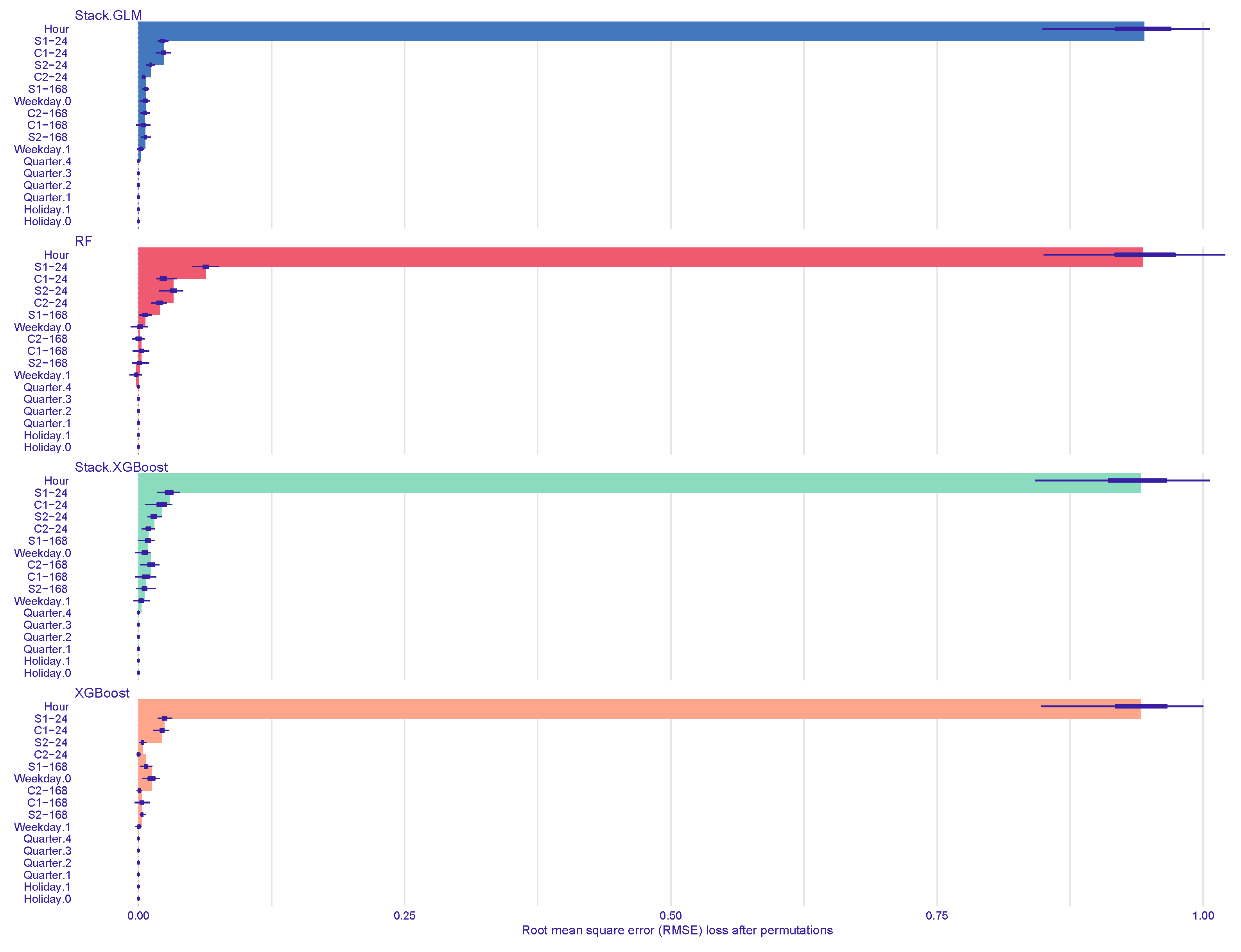
Based on the results reported in Table 4, the permutation importance of features is computed to examine the impact on predicting CDs. The permutation importance measures the decrease of the prediction performance of the model using the loss function after the values of the feature are randomly shuffled. If the value of the loss function calculated after shuffling is significantly greater than that calculated using the original dataset, it reveals that the variable is important. For the loss function, the root-mean-squared error (RMSE) loss function is considered with permutation 50 times. The result is plotted in Figure 6, which has the advantage of being easy to understand as it presents the most important variables in a single graph [22]. The x-axis in Figure 6 is the difference between the value of the loss function calculated after shuffling and that calculated using the original test dataset. It is interpreted as the larger the value, the more important the variable is. According to the argument, Hour is the most important and the Fourier daily terms are the next for all ML models. This means that the EV charging hour has the greatest impact on predicting CDs.

To find the best model among the considered predictive models, the prediction performance is compared through various perspectives including the prediction accuracy and scatter plot. Assuming that the prediction of $y_t^{{}^{\prime }}$ is ${\widehat{y}}_t$, the prediction error is defined as $e_t=y_t^{{}^{\prime }}-{\widehat{y}}_t$. The prediction error is an index for evaluating the reliability of the model, and the accuracy of the model can be measured based on this. The most commonly used numerical measures for the prediction accuracy are given by Shmueli et al. [23]:

• Mean of errors (ME): $\frac{1}{n}{\displaystyle \sum _{t=1}^n}{e}_t$;
• RMSE: $\sqrt{\frac{1}{n}{\displaystyle \sum _{t=1}^n}{e}_t^2}$;
• Mean of absolute errors (MAE): $\frac{1}{n}{\displaystyle \sum _{t=1}^n}\left|e_t\right|$;
• Mean of percentage errors (MPE): 100/n$\times {\displaystyle \sum _{t=1}^n}{e}_t/y_t^{{}^{\prime }}$;
• Mean of absolute percentage errors (MAPE): 100/n$\times {\displaystyle \sum _{t=1}^n}|e_t/y_t^{{}^{\prime }}|$.

The results for the predictive accuracy are reported in

Table 5. Accuracy measures for prediction.

	Statistical Model			ML Model
	DHR	STLM	BSTS	RF	XGBoost	Stack.XGBoost	Stack.GLM
ME	0.024	−0.064	0.200	−0.072	−0.015	−0.046	−0.035
RMSE	0.729	0.311	0.392	0.299	0.301	0.303	0.300
MAE	0.604	0.219	0.304	0.199	0.210	0.205	0.204
MPE	−2.168	−1.153	3.160	−1.805	−0.934	−1.483	−1.300
MAPE	11.691	4.239	5.570	4.107	4.285	4.233	4.203

, which indicates that the closer to zero the better, regardless of which evaluation indicator it is. This shows that, overall, the ML techniques based on the proposed hybrid strategy are more accurate in predicting than the considered statistical methods. More specifically, XGBoost is the best in terms of the ME and MPE, and RF is the best for the other. Additionally, to show the superiority of the proposed hybrid strategy, the results compared with the original ML method are presented in Figure 7. It reveals that the proposed hybrid strategy has generally better the prediction accuracy because the values obtained from it are closer to zero than those obtained from the original ML method, except for the MPE.

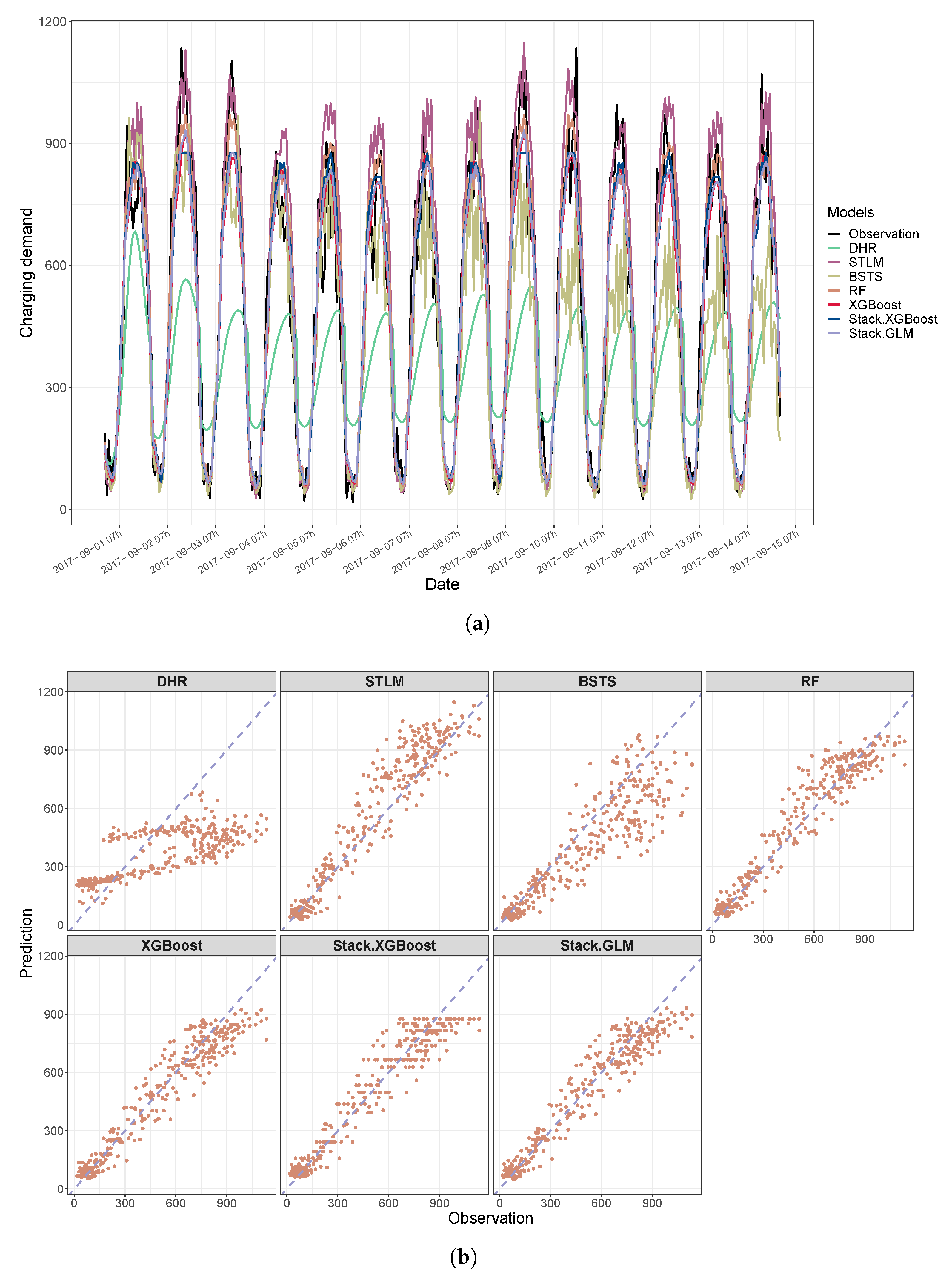
For visual examination, comparisons between the original test data and the predicted values converted into the original unit are further presented in Figure 8. All methods, except for DHR, provide similar values to the actual observations in Figure 8a. Figure 8b means that the closer the points are to the straight line, the better the prediction is. From this fact, we can see that all predictive models, except DHR, provide good predictive performance. Moreover, it can be seen that the ML techniques based on the proposed hybrid strategy provide better prediction results than the statistical methods such as STLM and BSTS.

4. Discussion and Conclusions

This paper proposes a hybrid strategy to resolve the drawback that the tree-based ML approach cannot capture the trend. The proposed hybrid strategy is to capture the trend component with traditional time series techniques such as the ARIMA model and then combine them with the ML techniques. Furthermore, unlike classical studies, the Fourier terms were considered as features to handle the seasonality.

To prove the validity of this approach, the proposed method was applied to the CD prediction problem of EVs. In addition, for better predictive modeling, Hour, Quarter, Weekday, and Holiday were considered as the feature through exploratory analysis, as well as the seasonality with the expression in the Fourier terms was considered as the feature. The superiority of the proposed method was demonstrated through comparison with the existing time series methods (DHR, STLM, and BSTS) and the original ML method.

Our results showed that the ML techniques based on the proposed hybrid strategy are superior to the existing statistical models, especially in RF. In addition, the prediction based on the proposed method was more accurate than that based on the original ML method. Based on these results, our proposed hybrid strategy has the benefit of helping to establish an electric power supply plan that can smoothly supply electric energy by accurately predicting the CD required as the supply of EVs increases. In addition, the proposed method can be applied to analyze time series data with trends and seasonality such as economy-related time series data, and its prediction performance is expected to be superior to the traditional time series and original ML methods.

Meanwhile, the DL method could not be performed because the amount of data used for training in this study was not large enough. In the future, when a vast amount of data is accumulated, it is expected that an excellent predictive model based on the DL technique can be developed through the combination of the proposed hybrid strategy and the DL technique.