Managing Perishability in the Fruit and Vegetable Supply Chains

Abstract

Spoilage reduction in fresh product supply chains is an important challenge and represents great opportunities for cost savings and reduced environmental and social footprints. The purpose of this paper is to identify the drivers of spoilage and to discuss how these insights can be used to reduce spoilage.We use panel data techniques to quantify the drivers of spoilage in the days-fresh category using daily spoilage and supply chain data (457,539 store-SKU level observations) for fresh fruits and vegetables at Switzerland’s largest retailer. We quantify to what extent inventory, promotions, delivery type, commitment changes, order variations, order cycle, and quality issues influence spoilage. We discuss the mechanisms through which inventory age and product standards impact spoilage of days-fresh products. Our novel findings underline the necessity for specialized supply chain processes, tracking inventory age and damage, and collaboration with supply chain partners in the management of this fundamental product category.

1. Introduction

Global food waste and loss cost is estimated to be USD 940 billion a year [1]. Waste and loss reduction in the food supply chain directly impacts the triple bottom line of companies [2] and represents opportunities for cost savings and reduced environmental and social footprints. Nonetheless, it remains a complicated problem, requiring solutions at all levels of the supply chain. The objective of this research is to identify the drivers of waste and losses in fruit and vegetable retailing and enable practitioners to implement the most effective solutions to this global problem. Throughout our study, we refer to waste, due to product degradation and expiration or other losses, as spoilage.

We use data from Migros to identify drivers of fresh fruit and vegetable spoilage. In 2015, Migros was the largest Swiss grocery retailer with 27.4 billion Swiss Francs in sales and a market share above 21%. Their main differentiator is relatively high product availability and large product assortment, where fruit and vegetable sales account for more than 10% of total supermarket sales. As with other retailers, fresh fruit and vegetables represent a highly competitive and high-margin product group that generates traffic flow into the store, requires high availability and specialized infrastructure, and involves seasonal portfolio changes. One of the fruit and vegetable store managers stated the following: “We can’t risk having empty shelves during the day. If a customer walks inside the store and doesn’t find the fruit or vegetable they are looking for, they turn back without buying anything at all and go to competitors.” As with all retailers who deal with fresh produce, perishability in this category is a major concern.

Challenges for fresh fruits and vegetables are both product-related and operational: product yields depend on climatic conditions, prices are volatile, suppliers are fragmented, the products are perishable and fragile (have temperature and handling requirements), and quality-control processes are laborious. Additionally, order and replenishment decisions are more critical than for weeks/months-fresh products due to short lifetimes. All of these factors drastically influence lead time, inventory, and overall costs.

For example, Target, the second-largest discount retailer in the US, is struggling to keep their perishable products fresh. While their fresh products represent USD 18.5 billion and make up one-fifth of their revenue, Target is suffering from high spoilage costs compared to the industry average. Their main problem is inventory aging due to a lack of store traffic for perishable products. To overcome the spoilage problem, they spent more than USD 1 million per store in 25 of their stores to increase traffic and better manage inventory, while increasing their replenishment frequency and offering localized products [3].

Spoilage occurs at all stages of the supply chain. According to a 2011 report by the Food and Agriculture Organization (FAO), in Europe, 45% of produced fruits and vegetables did not end up being consumed. Of those not consumed, 45% were lost at the agricultural stage; 30% were lost at post-harvest, processing, and distribution; and around 25% at the consumption stage [4]. Higher freshness at retailers could potentially reduce losses at the consumption stage. At the retailing stage, [5] identified loss rates as 3 to 5 percent of volume in fresh produce at best practice retailers, 6 to 8 percent among average performers, and 9 to 15 percent at under-performing retailers, due mostly to climate and long-distance transport. Although Migros can be defined as a best practice retailer according to this definition, spoilage for fresh fruits and vegetables represents a significant part of their annual profit in the fresh fruit and vegetables category.

To understand the major causes of spoilage, we collected supply chain data and conducted interviews with managers responsible for ordering fruits and vegetables at three levels of the supply chain: importers, DCs, and stores. We utilize 495,460 day-store-SKU level observations for 100 SKUs (products), from 128 stores over a four month period to show that spoilage is affected by inventory, promotions, delivery type, commitment changes in ordering, variation in orders at two supply chain echelons, order cycle, and quality issues at a statistically significant level.

Overall, excess inventory, order cycles, and variation, as well as longer delivery lead times, have the greatest impact on spoilage. As the number of days of inventory increases, inventory aging and sell-by constraints cause spoilage. We show that reducing the average inventory by half a day would reduce up to 40% of current spoilage costs. Smoothing store and distribution center (DC) orders by 50% each would also improve spoilage costs by 30%, while increasing the order frequency to daily orders would reduce spoilage costs by 17%. Direct deliveries are relatively infrequent and represent major improvement opportunities; increasing direct deliveries to 20% of total deliveries could reduce spoilage by 20%.

The contribution of this paper is two-fold. We add to the existing perishability literature by identifying and quantifying drivers of spoilage for days-fresh products in retailing. Second, we contrast the drivers of spoilage to those of weeks-fresh products. In performing this, we present an industry example of how collaborative forecasting could potentially fix incentive misalignments while reducing spoilage throughout the entire supply chain. For managers working in the days-fresh category, we recommend using specialized supply chain processes, tracking and quantifying inventory age and damage, and collaboration with supply chain partners to reduce inventory age.

The rest of the paper is organized as follows. In Section 2, we provide an overview of the literature. Section 3 describes the empirical settings in detail, i.e., the supply chain, ordering processes and perishability issues. In Section 4, we discuss our hypotheses for the drivers of spoilage. Section 5 describes the data in detail, and defines the variables. In Section 5.3, we discuss the empirical model used in the estimation. We present our empirical results in Section 6 and discuss their managerial implications. Finally, we conclude in Section 7 with a discussion of the limitations of our research and future research directions.

2. Literature Review

In our research, we consider the supply chain and retailing of fresh fruits and vegetables. Consequently, our research relates to the literature on perishable inventory. There are numerous studies on managing food perishability throughout the supply chain to increase freshness and value for supply chain entities. We first review studies that use mathematical models and subsequently those that use empirical data.

There is an increasingly rich body of studies that use mathematical modeling to study inventory models for perishable products, for which [6] provide an excellent review. Below we briefly review some of the seminal work in the field. Ref. [7] studied the impact of information sharing in relation to product age on a retailer’s profit in the grocery industry and found that the benefits are highest when demand variability and cost are high and product lifetimes are short. Focusing on product characteristics, ref. [8] introduced the marginal value of time of fresh produce to minimize lost value in the supply chain. Ref. [9] presented a method to determine dynamic order quantities for fresh food with positive lead time, FIFO or LIFO issuing policy, and multiple service level constraints. They showed that a constant-order policy might provide good results under stationary demand, short shelf-life, and LIFO inventory depletion. Ref. [10] optimized orders and prices for distributors and retailers of groceries and showed that coordination can benefit both parties. Ref. [11] quantified how backhauling and vertical differentiation can increase the retailer’s margin for local food, thus increasing the small local farmer’s competitiveness. Ref. [12] provided models to quantify the benefits of RFID technology in measuring and reducing waste for perishable foods.

Focusing on the grocery distribution chain, ref. [13] minimized total costs by clustering stores and selecting delivery patterns. Finally, ref. [14] optimized the replenishment frequency between a manufacturer and retailer considering both raw material and finished goods lifetimes.

We next analyze the literature on perishable inventory that uses empirical data. Ref. [15] segmented perishable products at a supermarket based on lifetime. They show that perishables have higher average sales, a smaller case pack size, lower coefficient of variation of weekly sales, lower potential delivery frequency, and a lower minimum inventory norm. Later, ref. [16] showed that perishables in retail have higher substitution rates compared to their durable counterparts and required cross-docking or direct delivery. In [17,18], the authors identified the causes of food waste in retailers in particular markets, with interviews; however, the weight of each cause is not quantified.

More recently, Ref. [19] studied in-store logistics processes for handling dairy products and found that strategic and tactical designs of in-store logistics processes lead to higher on-shelf availability and reduced obsolescence costs. Ref. [20] analyzed the impact of relative price discounts on product sales during promotions and provided guidance on forecasting promotional demand for perishable products. Ref. [21] highlighted the importance of shelf-life monitoring with innovative technologies. Refs. [22,23] showed that there is an important human aspect when dealing with perishability and that routines such as inventory rotation and aligning salesforce initiatives can greatly reduce product expiration.

The most relevant research for our study is [24], who explored the drivers of expiration for consumer packaged goods. They found that case size, inventory aging, negligence of shelf rotation, compliance to minimum order rules, manufacturer’s sales incentives, and forecast complexity are the main drivers. Although our objective is similar, there are fundamental differences between the latter study and our own. First, we focus specifically on fruits and vegetables, which are days-fresh products that are significantly different from weeks-fresh or months-fresh products in terms of lead times, inventory levels, sales, and quality [15]. Second, we analyze a panel of daily observations that allows us to capture drivers of spoilage for days-fresh products. Finally, fruits and vegetables can spoil within the sellable lifetime. Therefore, our scope extends from expiration to general spoilage, which includes product damage and heterogenous quality issues. A full contrast of results between days-fresh and weeks-fresh items is found in Section 6.

Due to the difference in products we observe, the setting of the supply chain, and the data we study, we further observed the impacts of the additional drivers that we identify, namely inventory quantity, delivery types, forecast updates, order variation at two supply chain levels, order cycle, as well as quality issues. We further account for product origin, packaging, season, and category.

As a result, to our knowledge, our study is the first to identify and quantify the drivers of waste and their economic impact for days-fresh perishable products using econometric modeling in the grocery supply chain.

3. Empirical Setting

In this section, we describe the retailer’s supply chain operations for imported fruits and vegetables. We do not consider local Swiss produce because the sourcing and ordering processes are different and product availability is often unpredictable.

The supply chain is shown in Figure 1. There are four players in the supply chain: producers, importers, DCs, and stores. Producers are located in more than 22 countries and are responsible for producing, harvesting, and packing the products for shipment. Migros works with five main independent and private importers based in Switzerland. Each importer is responsible for the delivery of certain categories of products to DCs. There are 10 independent DCs under the retail brand that assemble products into pallets based on store orders and dispatch them to stores on a daily basis. Each of the 650+ retail stores receive products before store opening every morning, except on Sundays. Store managers in fruit and vegetable sections are responsible for ordering, product display, and replenishment. They are evaluated on achieving sales targets, while reducing product discounts and waste. We next describe the ordering process.

The supply chain follows a pull ordering strategy. Every morning the stores place orders for the next store opening, based on factors such as weather, price, promotions, day of the week, week of the month, product quality, and product season. The order triggers the product flow from the DCs to the stores. The DCs pool the orders of their stores and pass them on to the importers, who deliver within one day. The importer typically holds less than half a day at the end of the day for safety, and DC holds close to zero days of inventory at the end of the day but due to transportation and ordering lead times, stores are replenished with products that are at least two days old. Tropical fruits are mainly shipped to Europe and ripened after arrival, with similar lead times from the importer onwards.

In order to guarantee product availability at stores, and account for the lead time difference between ordering at the stores and arrival at the DC, DCs send preorders. In other words, they send their order forecast, which can be modified during the week, to importers every Thursday for the following week. Preorders are based on historical data, and other factors that stores equally consider are as follows: weather, price, promotions, product, and time. However, the DCs’ preorders significantly deviate from the total daily orders placed by the stores. Consequently, the importers, who are contractually bound to deliver 100% of DC orders, need to cover for and speculate the difference between DC preorders and actual orders. They inflate or reduce their orders to the producers in advance based on historical data and experience.

There are two types of deliveries. In the first type, products first arrive from the producer to the importer and are subsequently sent to the DCs. In the second type, products are delivered directly from the producer to the DC. In the former, the preordering system is used with a possibility of updating orders during the week, which we call a commitment change. In the latter, preorders of the week cannot be changed and are offered a price discount from the retailer, just as in an advance purchase contract [25].

If the importers overorder, there are two potential scenarios. In the first, products are stored and subsequently sent to DCs in the following day, which reduces product freshness at the DC and store levels. At the DCs, it increases the likelihood of quality warnings issued from DCs to importers, while at the stores, it increases the likelihood of spoilage and customer returns. In the second scenario, the product quality is too low or product age is too high, causing products to be rejected at the DC. In this case, the importer finds an alternative buyer. If the products are not sold, they are donated, used as compost, turned into biofuels, or in rare cases incinerated.

The retailer differentiates itself by assuring a high in-stock level, while at the same time delivering fresh products. In addition, inadequate orders that increase inventory age and high service levels can indirectly cause spoilage in the supply chain. Date coding is used to increase the traceability of freshness: producers print the packaging date to individual consumer units to open cases. Ref. [7] show the benefits of sharing inventory age. The date is coded in a way that consumers cannot identify product age and avoids them from buying freshest products first, i.e., on a LIFO basis. The printed date code is used at two levels of the supply chain: DCs and stores. DCs check the date between their order and reception to and from the importer. This guarantees that the importer issues products on a FIFO basis and has not kept inventory for long durations. The store uses the date code to understand when the products should be removed from the shelves in order to reduce customer complaints and returns. Note that the date code is not digitally stored per item or by delivery, thus information on the age at sales or arrival cannot be accessed once the product leaves the supply chain echelon.

4. Drivers of Spoilage

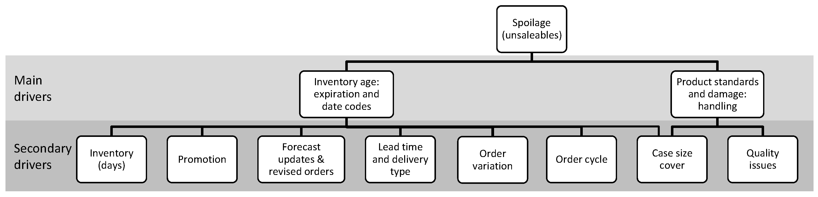
In this section, we motivate our hypothesis for the drivers of spoilage in stores. We classify the drivers of spoilage into two primary groups. The first is inventory age, which causes expiration due to the sell-by date (date codes) or insufficient quality due to degradation. The second is product damage or retailer’s product standards: size, color, sugar content, and packaging, among others. As in previous studies in the fruit and vegetable category, there are no continuous data available for inventory age or spoilage caused by product damage or visual/quality standards. The date code for packaged products is not digitally recorded per item or delivery; hence, information on the inventory age at sales or arrival is only available on print within a supply chain echelon. Damages or visual quality standards are not recorded in the system as a separate cause of spoilage. While the main drivers are not digitally available for analysis, it is possible to use other data that explain these two main causes and, therefore, spoilage. We formulate our hypotheses based on these drivers (shown in Figure 2), which are further discussed in the following subsections.

In our main analysis, we quantify the impacts of the secondary drivers shown in Figure 2 on spoilage. We first use an exploratory analysis to show the importance of inventory age for days-fresh items. In this additional analysis, we try to explore the impact of inventory age on spoilage solely due to sell-by dates using a simple simulation, similarly to [24], since we cannot quantify inventory age directly. We use a base-stock ordering policy under exponentially distributed sales on a FIFO basis, and different service levels at the retailer. We compare the results to real spoilage when there are no promotions (shown in Appendix C). Our results show that inventory age explains 100% of the spoilage at a 92% service level if we use an average of 4 days sell-by duration at the retailer. Spoilage increases as the allowable selling duration shortens and service level increases. Our result underlines the importance of inventory age for days-fresh products. Inventory age is clearly the main driver of spoilage for days-fresh products, which significantly differs from weeks-fresh products.

4.1. Inventory

For a fixed amount of sales, carrying more days of inventory at the store increases spoilage due product perishability [24]. Additionally, store managers are encouraged to hold maximum inventory at the display area and minimum inventory in the backroom to minimize handling time and inventory errors [26]. However, products in the display are subject to higher temperatures throughout the day, which increases the speed of maturity or decay [8]. Additionally, display area inventory is subject to more handling by customers, which increases damage and thereby spoilage. The role of inventory is discussed in Appendix E.

Hypothesis 1.

Spoilage increases with days of inventory at the store.

4.2. Promotions

Promotions have an important impact on sales of fresh products, causing sales to even triple for products such as mangoes, pineapples, and strawberries, as well as create traffic flow on the shop floor. High demand uncertainty, combined with other internal and external factors such as labor capacity or competitor pricing, might trigger inaccurate orders, which in turn increase inventory age. Ref. [20] state that promotions are responsible for a large part of the waste and stock-outs for perishable products since demand forecasting is more difficult for products on promotion.

Hypothesis 2a.

Spoilage increases with product promotions at the store.

With regard to forecasts and orders, our interviews with importers, DCs and store managers revealed that managers are more attentive when passing preorders and orders during promotions. Both DCs and importers use historical promotion data to forecast orders, and sometimes they even agree on forecasts and orders together. Regarding product quality, promotions often take place when the product is in the beginning of its season. It generally corresponds to the time when product quality and maturity is at its best and the supply is plentiful. In terms of delivery, products are often delivered with lower lead times due to less storage at the importer and DC. All these factors contribute to smaller inventory age or higher quality. In this regard, it has yet to be tested whether promotions increase or decrease spoilage.

Hypothesis 2b.

Spoilage decreases with product promotions at the store.

4.3. Forecast Updates and Revised Orders

DC weekly preorders (forecasts) are used to give an indication of what DC thinks the stores will order the following week. However, we observe significant differences between DC preorders and orders. If preorders turn out to be significantly higher than orders, importers store the products in order to send them the next day. Consequently, products are at least one day older, and we expect them to have higher spoilage rates in stores.

Hypothesis 3a.

Spoilage increases with commitment change at the DC.

Importers are responsible for delivering 100% of orders, which often requires them to over-order from producers. If the DCs order less from importers than what they originally preordered, it is likely that importers are left with extra inventory with little or no time left before they are required to deliver the products. In this case, the freshest products are sent to DCs, and the importers sell the remaining products to alternative buyers, or the products end up unsold. Consequently, commitment changes could result in higher product freshness and reduce spoilage at the store.

Hypothesis 3b.

Spoilage decreases with commitment change at the DC.

4.4. Lead Time and Delivery Type

Fresh products require short delivery times in order to maximize the duration in which the products can be sold and consumed [15]. While direct deliveries reduce transportation lead time, lower prices for direct deliveries might incentivize DCs to order the predefined minimum quantities and store extra inventory, even if their forecast is lower. This would consequently increase product age upon arrival at the store. Additionally, deliveries via importers take longer but allow DC orders to be modified and pooled, reducing the combined forecast errors and inventory age.

Hypothesis 4a.

Spoilage increases with direct deliveries from the producer to the DC.

Direct deliveries can reduce spoilage by reducing transportation lead time by one day. Moreover, they require DCs to allocate more time and care during ordering, as they cannot modify direct delivery orders should they observe demand changes during the week. An analysis is required to understand the impact of each delivery type.

Hypothesis 4b.

Spoilage decreases with direct deliveries from the producer to the DC.

4.5. Order Variation

Ref. [27] stated that smooth ordering patterns can dampen upstream demand variability. Demand variation is known to be one of the causes of the bullwhip effect [28,29], causing excessive inventory. For perishables, it indirectly causes spoilage due to expiration. In this case, DC order variation pushes importers to keep more safety stock due to their 100% service level rule. Higher days of inventory at the importer imply that products are delivered to stores later, i.e., with higher inventory age, and are prone to spoilage.

Hypothesis 5.

Spoilage increases with order variation at the DC.

Store product managers sometimes order with high variation even though demand is stable. This increases average inventory age since products are not transferred between stores. For example, if the real demand is 5 consumer units per day, and the orders follow a 0 and 10 pattern instead of a stable 5 units ordering pattern, the average age of the products is half a day higher. Additionally, high-orders variation over the course of a week may also make it harder for store managers to associate a specific day’s orders with its inventory and sales.

Hypothesis 6.

Spoilage increases with order variation at the store.

4.6. Order Cycle

Fruits and vegetables typically have short replenishment cycles or are prone to discounts given their short lifetimes [30]. In the case that we study, store managers have the option to order everyday (the delivery cycle is one day); however, they may decide to order less frequently to reduce handling efforts at the store. We expect average inventory age and, therefore, spoilage to increase when the order cycle increases.

Hypothesis 7.

Spoilage increases with the order cycle in which the product is shipped to the store.

4.7. Case Size Cover

Ref. [15] state that while average case size and the inventory norm for perishables is significantly smaller than for non-perishables, average case sizes for days-fresh and weeks-fresh products are the same. For weeks-fresh products, ref. [24] found that high case size cover (the days of demand that is covered by one case) is a driver for product expiry for consumer packaged goods. We test whether it is also valid for days-fresh products. Additionally, ref. [31] suggested that smaller case sizes can result in higher gross profit.

Hypothesis 8a.

Spoilage increases with the case size in which the product is shipped to the store.

On the one hand, the literature suggests that high case sizes result in higher spoilage rates due to higher inventory age. On the other hand, fruits and vegetables are delivered daily, have relatively small case sizes, and are fast-moving products. Furthermore, case sizes are often adjusted to sales and product characteristics. Small case sizes may cause too much handling in stores and DCs, subsequently damaging the products and causing spoilage. To evaluate which is more influential, we tested the opposing hypothesis.

Hypothesis 8b.

Spoilage decreases with the case size in which the product is shipped to the store.

4.8. Quality Issues

Importer deliveries to DCs are subject to a maximum allowable delay, which starts from the packaging date. If timing or product quality is inadequate, the DC issues a warning or penalty to the importer, which facilitates the measurement of importer performance in the long run. Reasons for quality warnings are inadequate sugar content, caliber, color, firmness, maturity, existence of bruises, rotting, molding, or other forms of damage. Inventory deterioration for perishables is generally modeled exponentially [8,32,33] and suggests that small quality issues at the DC are increasingly likely to result in spoiled products at the store the next day.

Hypothesis 9.

Spoilage increases with the gravity of quality issues at the DC.

5. Data Description, Variable Definitions, and Estimation Model

5.1. Data Description

In this section, we describe the data we collected from different supply chain levels and define our dependent and control variables.

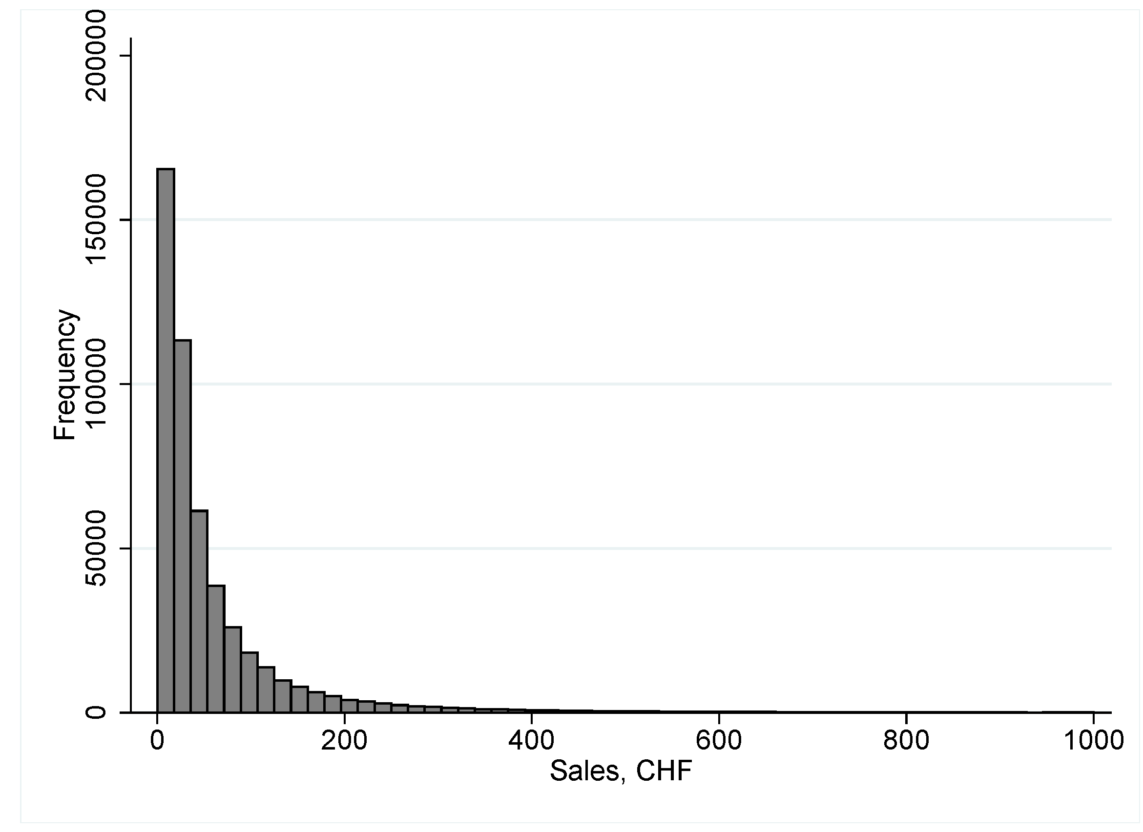
Our data contain 100 SKUs of imported fruits and vegetables that were sold for the first 4 months of 2016 in 128 Migros stores in the Geneva, Vaud, and Neuchâtel areas of Switzerland. For data extractability and computational efficiency, we use the top-selling 100 out of 272 SKUs, which represent more than 87% of the total sales volume for imported fruits and vegetables. Our dataset consists of 495,460 store-SKU level observations at daily granularity. Our data contain sales, delivery, promotion, spoilage, preorder, case type, origin, and sell-by data on a daily level. Additionally, with regard to qualitative data, we conducted interviews with importer, DC, and store managers.

5.2. Variable Definitions

We define our variables, in the order of the hypotheses, in what follows. The indices i, k, and t represent the SKU, store, and day, respectively. We additionally defined indices c and w for the DC and week.

• Spoilage or shrinkage performance in retailers is usually measured as a percentage of sales [5] to enable yearly comparisons and benchmark store performance. Therefore, we normalized spoilage as a fraction of sales as our dependent variable, measured as

  $$Spoilag{e}_{ikt}=\frac{Spoilagevalu{e}_{ikt}}{Sale{s}_{ikt}}.$$
• Inventory data are known to often be inaccurate [34,35,36]. Ref. [37] found that in their study, 65% of inventory records were inaccurate. Inventory data inaccuracy for fruits and vegetables occurs due to product code entry errors during weighing by customers at the display area or at the checkouts by employees. It is not uncommon to see negative inventory records. We adjust for such errors using inventory audit information, as well as corrections via manual changes at stores. We also additionally adjust for negative values and outliers due to obvious recording errors. (Inventory values can be high due to no display at the store for preparations for promotions or low sales on a particular day. Excluding inventory values that are high (only using observations for less than 10 days of inventory) does not significantly change the results). We use the definition of days of inventory outstanding and calculate the days of inventory as follows.

  $$Inventor{y}_{ikt}=\frac{Inventoryinstor{e}_{ikt}}{Sale{s}_{ikt}}.$$
• Promotion is a binary variable indicating whether the product is on promotion. National promotions are planned several months in advance, with product prices remaining constant for the entire week of the promotion. We denote it as $Promotio{n}_{it}$.
• Commitment change measures how much the DC’s order changes with respect to its preorder or forecast for deliveries via importers in one week. We calculate the change in commitment to preorders as follows.

  $$Commitmentchang{e}_{icw}=\frac{Preorderviaimporte{r}_{icw}-Orderviaimporte{r}_{icw}}{Orderviaimporte{r}_{icw}}.$$
  We do not observe spoilage spillover to the next week due to short product lifetimes and sell-by constraints and exclude a lag. If the orders are higher than the preorders, than the importer needs to provide extra products within a very short delay to the DCs. The newly arrived products are expected to be fresher (hence, the negative commitment change values), which occur in around 25% of the observations, and do not pose an issue for spoilage.
• Direct deliveries represent the fraction of direct deliveries to total deliveries in DC weekly preorders for each product. We measure direct deliveries as follows.

  $$Directdeliver{y}_{icw}=\frac{Directdeliverypreorder{s}_{icw}}{Totalpreorder{s}_{icw}}.$$
• DC order variation is the explanatory variable that measures whether volatility in DC orders influences spoilage, as suggested by the bullwhip effect [28]. We measure the daily coefficient of variation for the orders as follows.

  $$Distributioncenterordervariatio{n}_{ict}=\frac{{\sigma }_{ict}}{{\mu }_{ict}}.$$
  We use the rolling mean and standard deviation of orders over the past 7 days, calculated as ${\mu }_{ict}=\frac{1}{7}{\sum }_{j=(t-6)}^t{Order}_{icj}$ and ${\sigma }_{ict}=\sqrt{\frac{{\sum }_{j=(t-6)}^t{(Order}_{icj}-{\mu }_{ict}{)}^2}{7}},$ respectively. We use seven days since product origins, prices, and weekly forecasts are set on a weekly basis.
• Store order variation is calculated similarly to that of DCs, except we use the mean and standard deviation of daily store orders. Its impact is more direct compared to DC order variation since there is no dilution effect due to order pooling. Order variations are caused mainly by inaccurate forecasts and high employee turnover. We calculate the coefficient of variation for store orders as follows: $Storeordervariatio{n}_{ict}=\frac{{\sigma }_{ikt}}{{\mu }_{ikt}}.$
• Order cycle represents the average time between two orders for a given product. It is measured using the four-day rolling mean of ordering data in binary form: $Ordercycl{e}_{ikt}={\left(\frac{1}{4}{\sum }_{j=(t-3)}^{t}OrderBi{n}_{ikt}\right)}^{-1}$, where $OrderBi{n}_{ikt}$ is a binary variable representing the occurrence of orders for a given store-SKU-day. We use four days since it represents the average remaining product lifetime of products at the retailer. Further analysis shows that the results are the same following a 2–5 day rolling mean.
• Case size cover represents the days of demand (during the product shelf life) that is covered by one case. It is calculated as the quantity of consumer units in a case, divided by the demand during the product shelf-life. Consumer units are measured in kilograms or individual packages of a single product. We denote it as $Casesizecove{r}_i$.
• Quality issues indicates whether the product had a quality issue when it arrived at the DC. The quality problem is a score between 0 and 100, where 100 results in full product return, 0 results in acceptance with no reported quality issues, and values in between result in warnings with the score increasing with the gravity of the issue. We exclude products that scored 100 since they do not reach stores. It composes 13% of all quality issues and less than 0.08% of all deliveries within the study period. We denote it as $Qualityissue{s}_{it}$.

Our control variables are defined in

Table 1. Control variables.

Control Variable	Description
$Sale{s}_{ikt}$	Monetary value of sales of each SKU sold on a given day
$Demandvariatio{n}_{ikt}$	Coefficient of variation for sales for each product
$Sell-b{y}_i$	Maximum number of days each product is allowed to spend between shipping from the producer and sales at the stores
$Weigh{t}_i$	Binary variable indicating that the weight of each consumer unit is different. Consumer units are pre-packed, individually weighed, and priced according to their weight, with the price labeled on the package.
$Ne{t}_i$	Binary variable indicating that the product is sold in a net, such as for oranges. Each consumer unit net weight is identical.
$Opencas{e}_i$	Binary variable indicating that the product is sold in an open case, where consumers choose the units they wish to purchase, and pay by weight.
$Singleuni{t}_i$	Binary variable indicating that the product is sold in single units, such as for mangoes, avocados and cucumbers. For these products, individual product appearance is of higher importance.
$Stor{e}_k$	Binary variable for store k.
$Distributioncente{r}_{ik}$	Binary variable for DC c.
$Importe{r}_{ik}$	Binary variable for importer p.
$Categor{y}_i$	Type of product. For example, all tomatoes fall under the same category, yet there are multiple varieties. We expect SKUs in the same category to have similar spoilage fractions in most cases.
$Origi{n}_{iw}$	Country of origin of the product. There are over 22 origins in our dataset. The product origin may change based on ripening in different countries at different times.
$Category\times wee{k}_{iw}$	Binary variable controlling for each product category-week combination. It can be interpreted as the season of the product.
$Mont{h}_t$	Month of the year
$Dayofwee{k}_t$	Day of the week

. We provide summary statistics for our variables in

Table 2. Summary statistics.

Variable	Mean	Std. Dev.	Min.	Max.	N
Spoilage	0.038	0.266	0	42.523	487,142
Independent variables
Inventory (days)	2.46	3.07	0	395.60	487,144
Promotion	0.15	0.36	0	1	495,460
Commitment change	0.19	0.69	−1	3.46	489,407
Direct delivery	0.03	0.06	0	1	495,460
DC order variation	0.39	0.22	0	2.65	482,449
Store order variation	0.87	0.54	0	2.65	482,449
Order cycle	1.54	0.75	1	4	469,347
Case size cover	0.11	0.19	0	10	478,781
Quality issues	1.53	6.02	0	78.59	495,460
Control variables
Sales (CHF)	61.35	103.06	0	4758	495,460
Demand variation	0.49	0.21	0	3.32	484,641
Sell-by (days)	9.41	3.24	5	15	495,460
Weight	0.27	0.44	0	1	495,460
Net	0.14	0.34	0	1	495,460
Open case	0.26	0.44	0	1	495,460
Single unit	0.22	0.41	0	1	495,460

.

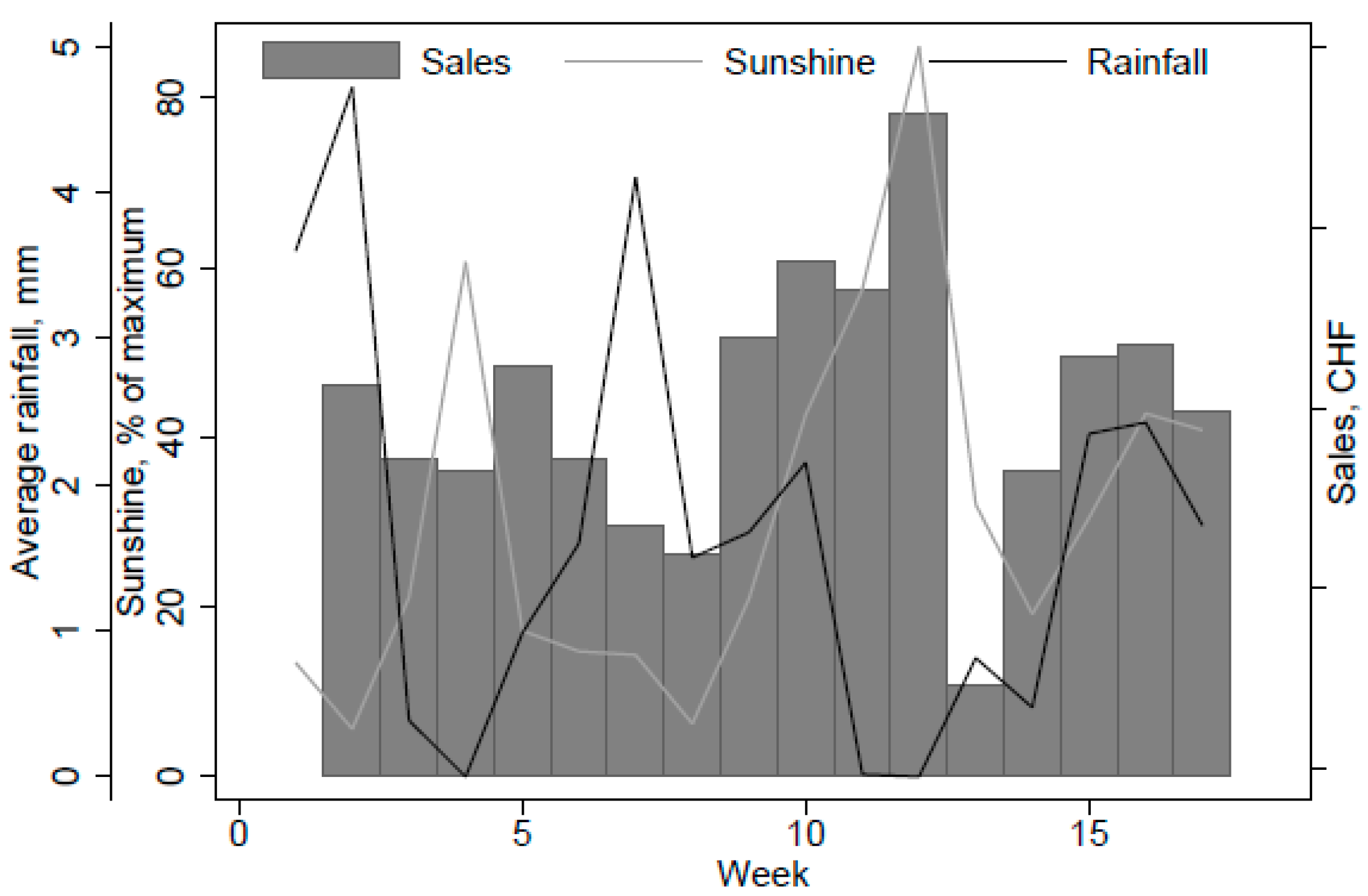
Weather has an important influence on sales. We use weekly weather data to measure its impact on weekly sales in the DCs. We obtain data for rainfall and sunshine from three weather stations located in each of the three regions corresponding to DC locations. We use average weekly rainfall, in millimeters, and weekly sunshine as a percent of the maximum. Our results show that, on average, each extra percentage of sunshine increases sales by more than 1800 Swiss Francs, while each extra millimeter of rainfall costs more than 16,000 Swiss Francs per DC. However, we exclude weather as a control variable for three reasons. First, DC and store managers already account for weather in their orders. As a result, weather does not influence spoilage as a percentage of sales. Second, we control for sales. Third, the cool chain is maintained during transportation and storage up until the displays are in the store.

Table A1. The impact of weather on sales, in CHF.

Weekly Sales	OLS
Weekly Rain (mm)	−16,376 ***
	(53.62)
Weekly Sun (%)	1823 ***
	(8.840)
Constant	446,415 ***
	(586.4)
Observations	495,460
R-squared	0.730
N	495,460
r2_a	0.730

Standard errors in parentheses. *** p < 0.01.

and Figure A4 show the impact of weather on sales.

Switzerland has the highest organic product consumption per capita in the world, with Migros representing a quarter of organic product sales in Switzerland [38]. We observe no significant difference between spoilage in organic and conventional fruits and vegetables at the stores. According to one of the importers we interviewed, which only imports organic products, “Organic products mostly spoil at production and harvesting stages. Only a fraction of the remaining harvest meet the visual requirements and are transported abroad”, which explains our finding.

In our paper, we do not include store order propositions of automatic ordering systems, as in [39] for two reasons. First, the propositions do not include factors such as weather, promotions, price changes, or long-term historical data. Second, our interviews revealed that they are not used by store managers and that an improved proposition system is currently under development.

5.3. Estimation Model

Our model covers all nine variables associated with our hypothesis: inventory, promotion, commitment change, direct delivery, DC and store order variations, order cycle, case size cover, and quality issues.

$$\begin{array}{cc}\hfill Spoilag{e}_{ikt}=& \alpha +{\beta }_{1}Inventor{y}_{ikt}+{\beta }_{2}Promotio{n}_{it}+{\beta }_{3}Commitmentchang{e}_{icw}\hfill \\ \hfill & +{\beta }_{4}Directdeliver{y}_{icw}+{\beta }_{5}Distributioncenterordervariatio{n}_{ict}\hfill \\ \hfill & +{\beta }_{6}Storeordervariatio{n}_{ikt}+{\beta }_{7}Ordercycl{e}_i+{\beta }_{8}Casesizecove{r}_i\hfill \\ \hfill & +{\beta }_{9}Qualityissue{s}_{it}+{\beta }_{10}Sale{s}_{ikt}+{\beta }_{11}Demandvariatio{n}_{ikt}\hfill \\ \hfill & +F_{ik}+T_t+S_{iw}+{ϵ}_{ikt}\hfill \end{array}$$

$F_{ik}$ is the vector of covariates for time-invariant fixed effects for all store-SKU combinations, namely the sell-by constraint, product category, package characteristics weight, net, open case and single unit, store, distribution center, importer, and all other factors that do not change over time.

Our analysis focuses on the fixed-effects model; however, we also show the random effects and OLS models. We use the remaining control variables given in Table 1 in the random effects and OLS specifications. $T_t$ is the time-specific fixed effects for the month and the day of the week. $S_{iw}$ represents the covariates for origin and $Category\times wee{k}_{iw}$ fixed effects. ${ϵ}_{ikt}$ denotes the error term for the observation for product i in store k and day t. While some relationships between the secondary drivers exist, the correlations are very low and further analysis show that there are no strong mediating/moderating relationships.

6. Results and Discussion

In this section, we present the results of our estimation model. We first discuss and compare the impact of each variable on spoilage and present additional tests to show the effects of time-invariant variables thereafter. Second, we discuss generalizability and show the robustness of the results.

6.1. Estimation Model Results

Table 3. Estimation model results.

Spoilage	Fixed Effects	Random Effects	OLS
Inventory	0.0238 ***	0.0238 ***	0.0240 ***
	(0.00429)	(0.00421)	(0.000131)
Promotion	−0.0229 ***	−0.0213 ***	−0.0205 ***
	(0.00354)	(0.00341)	(0.00137)
Commitment change	−0.00899 ***	−0.00750 ***	−0.00617 ***
	(0.00107)	(0.00102)	(0.000696)
Direct delivery	−0.0335 ***	−0.0301 ***	−0.0297 ***
	(0.0112)	(0.00877)	(0.00918)
Store order variation	0.0254 ***	0.0239 ***	0.0216 ***
	(0.00341)	(0.00298)	(0.000939)
DC order variation	0.00905 ***	0.0105 ***	0.0114 ***
	(0.00344)	(0.00326)	(0.00214)
Order cycle	0.00947 ***	0.00909 ***	0.00869 ***
	(0.00141)	(0.00129)	(0.000613)
Case size cover	−0.00929	0.00722	0.0172 ***
	(0.0417)	(0.0192)	(0.00353)
Quality issues	0.000305 ***	0.000329 ***	0.000346 ***
	(0.000109)	(0.000107)	(7.05$\times {10}^{-5}$)
Sales	−0.000103 ***	−8.42$\times {10}^{-5}$ ***	−7.19$\times {10}^{-5}$ ***
	(1.21$\times {10}^{-5}$)	(9.54$\times {10}^{-6}$)	(4.94$\times {10}^{-6}$)
Demand variation	0.00952 *	0.00708	0.00756 ***
	(0.00548)	(0.00573)	(0.00233)
Open case		−0.0239 ***	−0.0318 ***
		(0.00924)	(0.00411)
Single unit		−0.0383 ***	−0.0462 ***
		(0.0112)	(0.00579)
Weight		−0.0316 ***	−0.0370 ***
		(0.00863)	(0.00371)
Net		−0.0123	−0.0209 ***
		(0.00970)	(0.00445)
Store-SKU fixed effects included	Yes	No	No
Other controls included ${}^a$	Yes	Yes	Yes
Constant	−0.152 ***	0.131 ***	0.145 ***
	(0.0359)	(0.0281)	(0.0282)
Observations	457,539	457,539	457,539
R-squared	0.075		0.098
Number of ID	9268	9268
Within R-squared	0.0751	0.0749	.
Between R-squared	0.00862	0.239	.
Overall R-squared	0.0405	0.0979	.
F	6.244	.	71.36

Robust standard errors in parentheses. *** p < 0.01, * p < 0.1. ^a Controls: sell-by constraint, product category, month, day of the week, origin, and Category × week.

shows the estimated coefficient for the estimation model using fixed effects, random effects, and ordinary least squares models. The standard errors are given in parenthesis. Each variable, except for Case size cover which is related to Hypothesis 8 and is rejected, consistently increases or decreases spoilage for all three specifications. However, the dimension and significance level varies. The Hausman test [40] indicates that the difference between the specifications are significant, and that the random effects and OLS are inconsistent. Hence, we use the results from the fixed effects model to drive our initial analysis and compare the impacts of each variable.

We discuss the results for the hypotheses in what follows. The estimates of the fixed effects model show that Hypotheses 1, 5, 6, 7, and 9 are all strongly supported at the $p<0.01$ level: more days of Inventory (0.0238), Order variations at stores (0.0254) and DCs (0.00905), longer Order cycles (0.00947), and Quality issues (0.00031) at the DC all increase spoilage, as expected. Hypothesis 8 is not supported by our data.

Hypotheses 2b, 3b, and 4b are supported by our data at a $p<0.01$ level. We discuss the results in detail in what follows. In Hypothesis 2, we tested whether Promotions increase (2a) or decrease (2b) inventory age and spoilage. Hypothesis 2b is supported at the $p<0.01$ level and shows that spoilage decreases with product Promotions at the store (−0.0229). This result is different from the findings of [20] and can be explained with several reasons. First, we analyze fast-moving days-fresh products. Second, orders tend to be passed in advance and with higher care due to sales targets and the use of historical promotion data to forecast sales for each promotion. Third, we control for sales. Even so, we lack inventory age data, and promotions can highly influence these. Finally, early promotion planning enables higher product quality and longer lifetimes thanks to improved harvest timing. With respect to damages, promotions may involve special packaging that better protects the products.

In Hypothesis 3, we tested whether Commitment change increases (3a) or decreases (3b) inventory age and spoilage at the store. Hypothesis 3b, supported at the $p<0.01$ level, reveals that Commitment changes between preorders and orders reduce spoilage (−0.00899). There are three main explanations. First, DCs update their orders after observing demand at the beginning of the week. Better forecasting together with higher demand at the end of the week reduces both inventory age and spoilage. The second explanation is that importers order based on preorders, but due to date codes or inventory aging, the products never reach the stores. According to interviews with one of the importers: “Even though the quality of the product is adequate, date codes prevent us from selling the products to DCs, forcing us to look for alternative buyers. It is especially challenging when products have high volumes or when the retail brand is already in the label”.

The third and more likely explanation is that importers do not rely on preorders but rather on their own forecasts. The importers do not receive sales information and are obliged to deliver 100% of retailer orders despite an average 3 to 4 day transportation lead time. While the retailer benefits from this situation, the importer suffers the consequences. As far as DC preorder accuracy is concerned, one of the importers stated that “Strictly following preorders would be disastrous”. Lack of trust [41] between the importer and DCs presents opportunities to improve.

Both parties could potentially benefit from collaborative forecasting [42] and, as a consequence, reduce inventory age throughout the supply chain, as well as avoid potential bullwhip effects. However, the parties would first need to strengthen their relationship. As [43] pointed out, “Partially observed demand information is more difficult to use … because of the difficulties in building the needed customer–manufacturer relationship as well as the difficulty of transforming partial demand information into useful data”.

In Hypothesis 4, we tested whether Direct delivery increases (4a) or decreases (4b) inventory age and spoilage at the store. Hypothesis 4b, also supported at the $p<0.01$ level, shows that the benefits of Direct delivery overcomes the advantages of pooling DC orders. One of the benefits of direct deliveries is an extra day of freshness (−0.0335). According to one of the importers we interviewed, “An extra day of freshness in our operations would create an enormous reduction on spoilage”. Direct deliveries also improve ordering, since DCs cannot change their orders during the week.

In Hypotheses 8, we tested whether Case size cover increases (8a) or decreases (8b) spoilage, arguing that large case sizes could increase spoilage due to inventory age, and small case sizes could increase spoilage due to more handling. Both hypotheses are rejected by our data and show that Case size cover does not influence spoilage at a statistically significant level. We believe that the reasons are product type and retailer practice related. We focus on fruits and vegetables, which are days-fresh products that are very fast-moving, as opposed to most weeks-fresh products or other days-fresh products with low demand. Regarding retailer practice, we observe low average case sizes, which are well adjusted to sales. The average case size in our data covers only 11% of demand during the lifetime of the SKUs. We recommend further analysis on the effect of case size cover on spoilage for various days-fresh products in different retailer settings.

We now contrast our results with the results for weeks- or months-fresh products presented in [24]. Overall, the studies only overlap on three main hypothesis, of which one in each study is not supported. In both studies, inventory age significantly increases spoilage; however, the relative effect to other estimates is much higher for days-fresh products. The hypothesis that larger case sizes increase spoilage was not supported for days-fresh products. Following a FIFO policy through by increasing rotation, or reducing order cycles in our case, reduces spoilage for days-fresh products. This hypothesis is not supported for weeks-fresh products.

Following larger order quantities reduces spoilage for weeks-fresh products, with less frequent deliveries requiring less transportation costs. However, this hypothesis is not applicable for days-fresh products as store managers are encouraged to order daily, as the delivery and transportation occurs everyday to keep products as fresh as possible. Likewise, giving commissions on sales to store managers via sales incentives are not applicable in our study. Sales and spoilage performance are tracked in parallel. Finally, [24] show that forecasting more store-product combinations per sales manager increases spoilage. The number of store-product combinations does not vary over our period of analysis, thus the complexity remains the same. We control for the product, store, and DC, since only one manager in each specific store or DC is in charge of ordering. Additionally, we observe that larger DCs are generally better at forecasting.

In addition to the hypotheses analyzed above, we include the days of inventory, commitment changes, delivery types, order variations, promotions, and quality issues into our analysis. These have not been explicitly studied for weeks-fresh items.

6.2. Economic Impacts and Managerial Insights

Our results can be used by managers to prioritize the improvements in the fresh product supply chain. In this section we compare the economic impact of the drivers on spoilage costs and summarize the managerial insights. Figure 3 shows the economic impacts of improving the drivers of spoilage.

We compare the impact of feasible targets at stores and DCs. Currently, the stores carry almost 2.5 days of inventory on average, which implies that if they stopped ordering, they are expected to stock out after 2.5 days. Part of the reason is due to aesthetic reasons to keep the shelf display full at the end of the day. We find that reducing Inventory at stores by half a day of sales, which represents only 20% of current inventory levels, would have the greatest impact on spoilage (up to 40%) without major compromise in service levels. This can be implemented by adjusting employee incentives to manage inventory and by introducing new display methods that make the shelf look fuller. We recommend managers to track inventory and service levels simultaneously in this category in order to optimize product freshness and reduce spoilage costs without damaging consumer loyalty.

Reducing the order cycle to one day, which is the current replenishment cycle, can reduce spoilage by 17%. Similarly, order variation at stores and DCs provide improvement opportunities in the order of 15% each. We note that more frequent orders with less volatility may also represent higher handling requirements at stores. Order variation and cycles can be reduced by tracking accurate inventory information, training personnel for better forecasting or building an automated ordering system that considers factors such as time, weather, and substitution simultaneously. Consequently, rationing and shortage gaming can also be eliminated.

Direct deliveries are currently infrequent and represent a significant lever for improvement. Our findings show that reducing transportation lead time is crucial for the days-fresh category. An increase to 10% of total deliveries would reduce spoilage costs by 8%. However, after a certain percentage increase in direct deliveries, volumes may not be sufficient to fulfill direct delivery transportation fill rates. This would result in excess orders, which would subsequently cause spoilage at DCs.

Promotions and quality issues at the DC have the least impact on store spoilage. We do not include case cover, as the hypothesis is not supported. We also exclude commitment change, as we believe commitment changes could potentially be pushing spoilage to importers, while also reducing trust within the supply chain in the long run.

To discuss time invariant factors, namely product packaging, we show the results of the Mundlak approach [44,45]. The results are shown in Appendix D. We find that the $Weight$ type packaging significantly reduces spoilage, possibly due to higher product protection compared to other packaging types. They are often pre-packaged with cardboard or hard plastic.

6.3. Generalizability

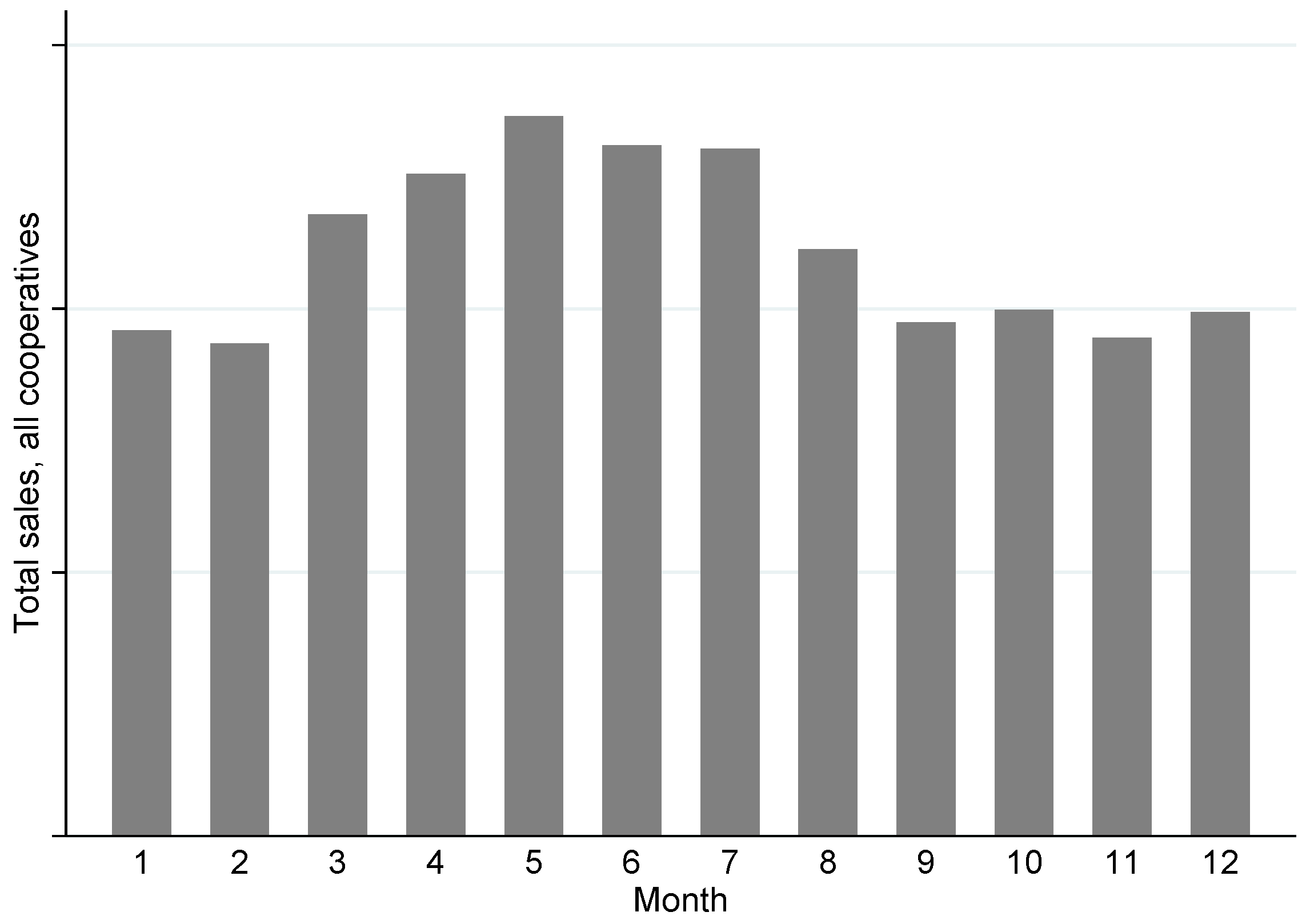
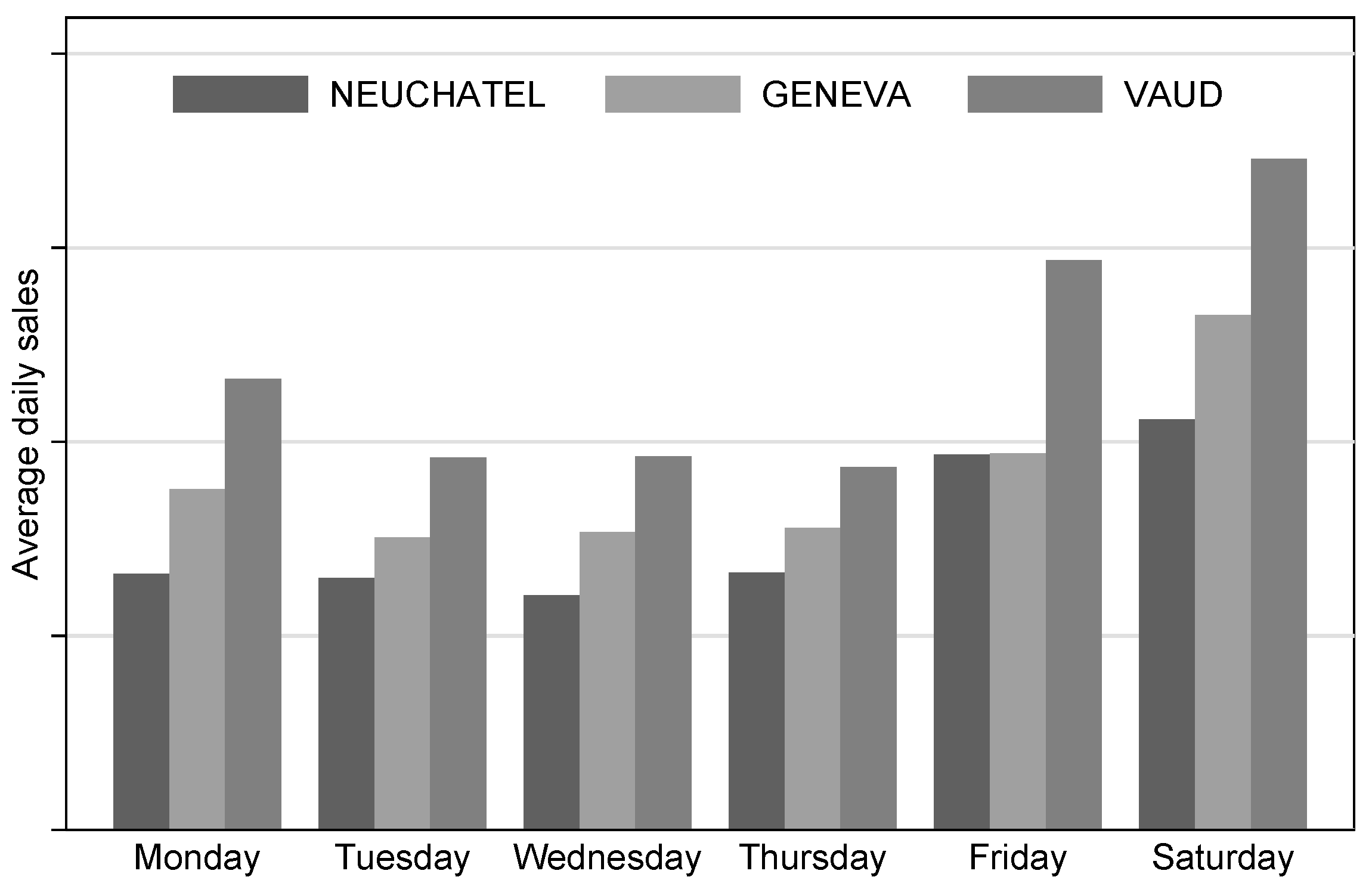
In this section, we discuss the generalizability of our results by analyzing sales patterns, aggregating data on a weekly and monthly basis, and using SKU categorization based on sell-by limits.

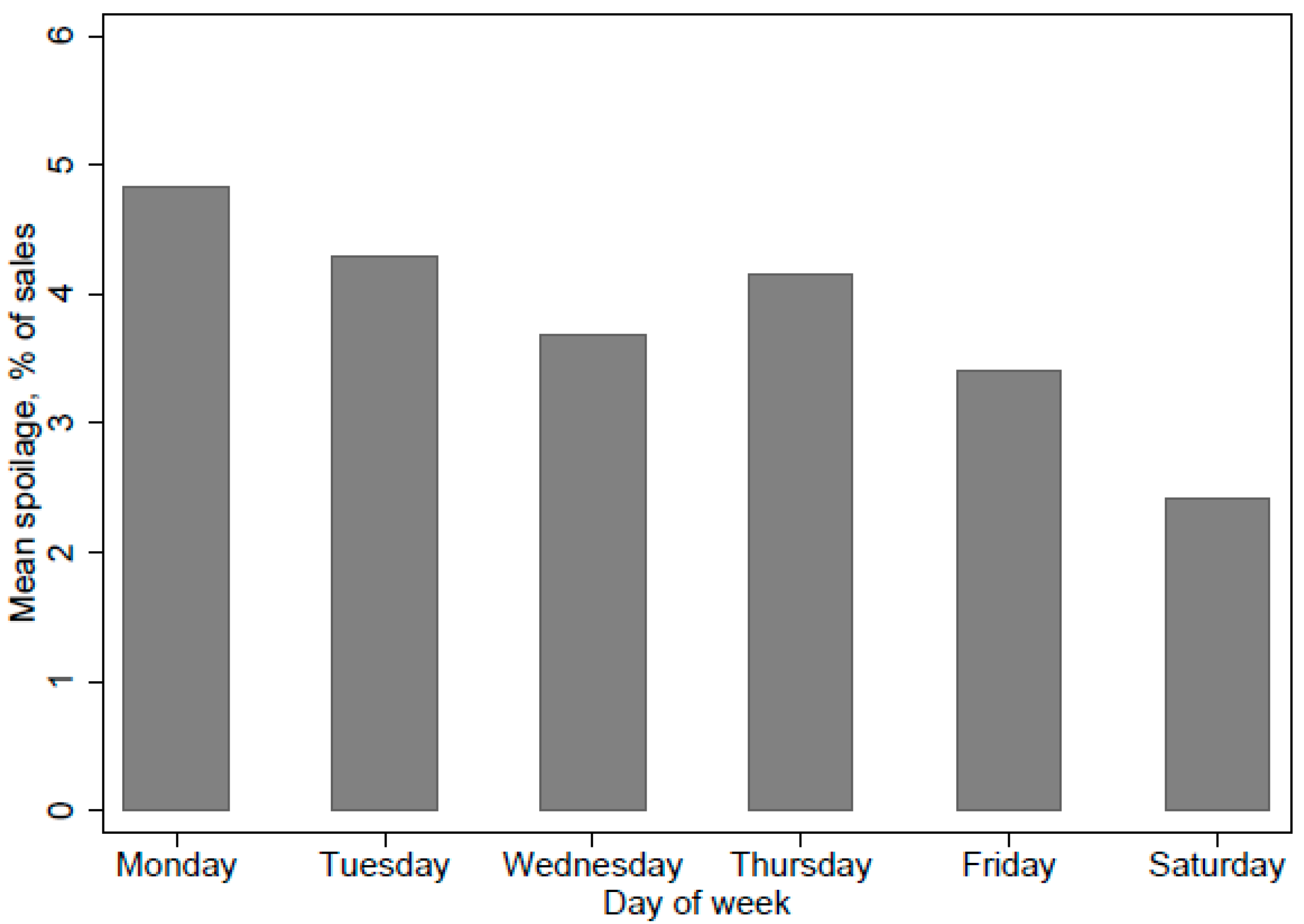
First, we show that weekly and yearly patterns of sales are similar to the findings in the literature. Namely, our weekly sales pattern shown in Appendix A is similar to the aggregate seasonality sales pattern presented in [39]. Sales are at the lowest during the middle of the week and increase toward the weekend. Likewise, the yearly sales pattern is similar to that of [24], where the authors use 13 periods of 4 weeks each.

Finally, we group SKUs based on sell-by limits of products. The first group, highly perishables, includes SKUs that have a maximum sell-by date, as of packaging or shipment from the producer, of 9 days. SKUs in this group include strawberries (5 days), spinach (6 days), grapes (7 days), and tomatoes (8 days). The second group, moderately perishables, includes SKUs with a sell-by date that is above 9 days: for example, oranges, plums, kiwis, and pineapples.

Table 4. Results for highly perishable SKUs and moderately perishable SKUs.

Spoilage	Fixed-Effects	Fixed-Effects
	Highly Perishables	Moderately Perishables
Inventory	0.0262 ***	0.0211 ***
	(0.00488)	(0.00765)
Promotion	−0.0233 ***	−0.0233 ***
	(0.00411)	(0.00606)
Commitment change	−0.0120 ***	−0.00467 ***
	(0.00145)	(0.00152)
Direct delivery	−0.0298 **	−0.0436
	(0.0118)	(0.0334)
Store order variation	0.0388 ***	0.0138 ***
	(0.00548)	(0.00407)
DC order variation	−0.00609	0.0240 ***
	(0.00506)	(0.00528)
Order cycle	0.0132 ***	0.00618 ***
	(0.00252)	(0.00117)
Case size cover	−0.0415	0.0488
	(0.0560)	(0.0301)
Quality issues	0.000348 **	0.000108
	(0.000135)	(0.000125)
Sales	−0.000101 ***	−0.000102 ***
	(1.57$\times {10}^{-5}$)	(1.85$\times {10}^{-5}$)
Demand variation	0.00724	0.0110
	(0.00639)	(0.00953)
Store-SKU fixed effects included	Yes	Yes
Other controls included ${}^a$	Yes	Yes
Constant	−0.138 ***	−0.0343
	(0.0357)	(0.0238)
Observations	253,508	204,031
R-squared	0.077	0.075
Number of ID	6023	3245
Within R-squared	0.0775	0.0747
Between R-squared	0.00192	0.107
Overall R-squared	0.0313	0.0767
F-statistic	6.358	5.861

Robust standard errors in parentheses. *** p < 0.01, ** p < 0.05. ^a Controls: sell-by constraint, product category, month, day of the week, origin, and Category × week.

shows results of estimation model for the two SKU groups. It is clear that SKUs in the highly perishable group are more sensitive to the drivers of spoilage (the magnitude of the coefficients are consistently higher for highly perishables). Inventory, Promotion, Commitment change, Store order variation, and Order cycle are statistically significant for both SKU groups. However, Direct delivery and Quality issues are only statistically significant for the highly perishable group, which supports the fact that the drivers for spoilage vary between fresh products (days-fresh and weeks-fresh) and even partially within the days-fresh category.

The preordering system used in our case represents partial demand information transfer that is common to many supply chains [43]. To test whether having the preorder system influences our results, we use yearly data of all 10 DCs and 5 importers. One DC out of ten and one importer out of five do not use preorders at all. They represent 25% of total observations. We create a binary variable for having preorders and found that preorders alone do not explain spoilage per se.

7. Conclusions

Spoilage in fresh food supply chains is a crucial issue, with both economic and environmental impacts on all its entities. The stores struggle with unpredictable demand; the DCs struggle with order inaccuracy and product quality; importers struggle with preorder inaccuracy and product handling; producers need to know how much crop they need to produce multiple months in advance. Given these issues, a detailed analysis of the main causes of spoilage is essential to identify effective solutions.

There is relatively little empirical literature that studies the drivers of spoilage for days-fresh products. We contribute to the existing literature by identifying drivers for spoilage in the days-fresh category and by presenting the differences from weeks-fresh products. We use daily spoilage and supply chain data from Switzerland’s largest retailer to drive an econometric analysis and conduct multiple interviews at three supply chain levels.

We show that excess inventory, promotions, delivery type, commitment changes in ordering, order variations at two supply chain echelons, order cycle, and quality issues all impact spoilage at a statistically significant level. Our economic analysis shows that inventory, order variation, delivery lead time, and collaboration among supply chain entities can enable the most effective improvements in spoilage costs. We further quantify the improvement potential of each driver on spoilage for days-fresh products, while categorizing them into two primary causes: inventory aging and product standards or damage.

We provide three main managerial insights that can improve spoilage performance in the days-fresh category. First and foremost, days-fresh products require specialized supply chains that address the perishability requirements: A single-transport ordering, replenishment, and sales process for all products is not adequate to obtain the high service-level and low spoilage objective. Managers should prioritize direct deliveries to reduce transportation lead times in the upstream supply chain, while using live sales information to reduce information lead time downstream.

Second, collaboration in the supply chain can reduce spoilage and produce substantial economic savings while also improving environmental performance; therefore, we urge managers to leverage producer and supplier relationships to improve forecasting, visibility, and operations within the entire supply chain. Collaborative forecasting and ordering, particularly when there are few suppliers, can improve initial forecasts and reduce commitment changes. While commitment changes, i.e., forecast updates, are beneficial for retailers, they are potentially detrimental to retailers’ relationships with entities in their upstream supply chain due to long transportation lead times.

Finally, we recommend tracking and quantifying inventory age and damage throughout the supply chain. Collecting data for quality and inventory age can enable the identification of supply chain weaknesses, while personnel training for inventory management in the downstream supply chain can reduce order variation and order cycles, which in turn reduce inventory age and spoilage.

On a more general note, we recommend implementing automatic ordering processes that use advanced data techniques at the retailer level, which are becoming more prominent [46] despite the high setup costs. An automatic ordering system that uses live sales data would reduce the upstream supply chain responsibilities mainly to ensuring quantity, quality, adequate logistics, and data integration, while reducing downstream system responsibilities to ensure data quality and collaboration within the supply chain. For Migros, it would eliminate the one-hour daily ordering task in more than 600 stores and focus store manager efforts for in-store replenishment and improved display, particularly during promotions.

There are some limitations to our study. First, data could be partially inaccurate due to recording errors at retailers [34,35], which we try to correct using inventory correction data at the store level and by eliminating obvious data errors. Second, there is no recorded data for inventory age, which is the main driver for spoilage in the fruit and vegetable category. We simulate spoilage due to expiration and find that it explains a significant amount of spoilage. Third, there is a lack of data for initial product quality, perishability, and taste, which are very heterogeneous over time, which explains the relatively low explanatory power of our model. Fourth, we do not consider substitution due to the lack of information on substitution relationships between products and high number of products. Finally, the data we used were collected during four months. As the context, we are studying is highly seasonal, it is not certain that our results can generalize to other seasons.

We recommend analyzing the effects of product packaging on spoilage for a wide variety of products with multiple packaging types as a future work avenue. Additionally, it has yet to be tested whether product origin or local production has a significant influence on spoilage through inventory age when controlled for quality. Other promising avenues include the effect of collaborative [36] and improved forecasting [47], multiple daily deliveries [48,49], and the impact of promotions in substitute products on spoilage in the days-fresh category.