
How COVID-19 Affected GHG Emissions of Ferries in Europe


Abstract
:
1. Introduction
2. Literature Review and Research Questions
2.1. Research Questions
- Q1.
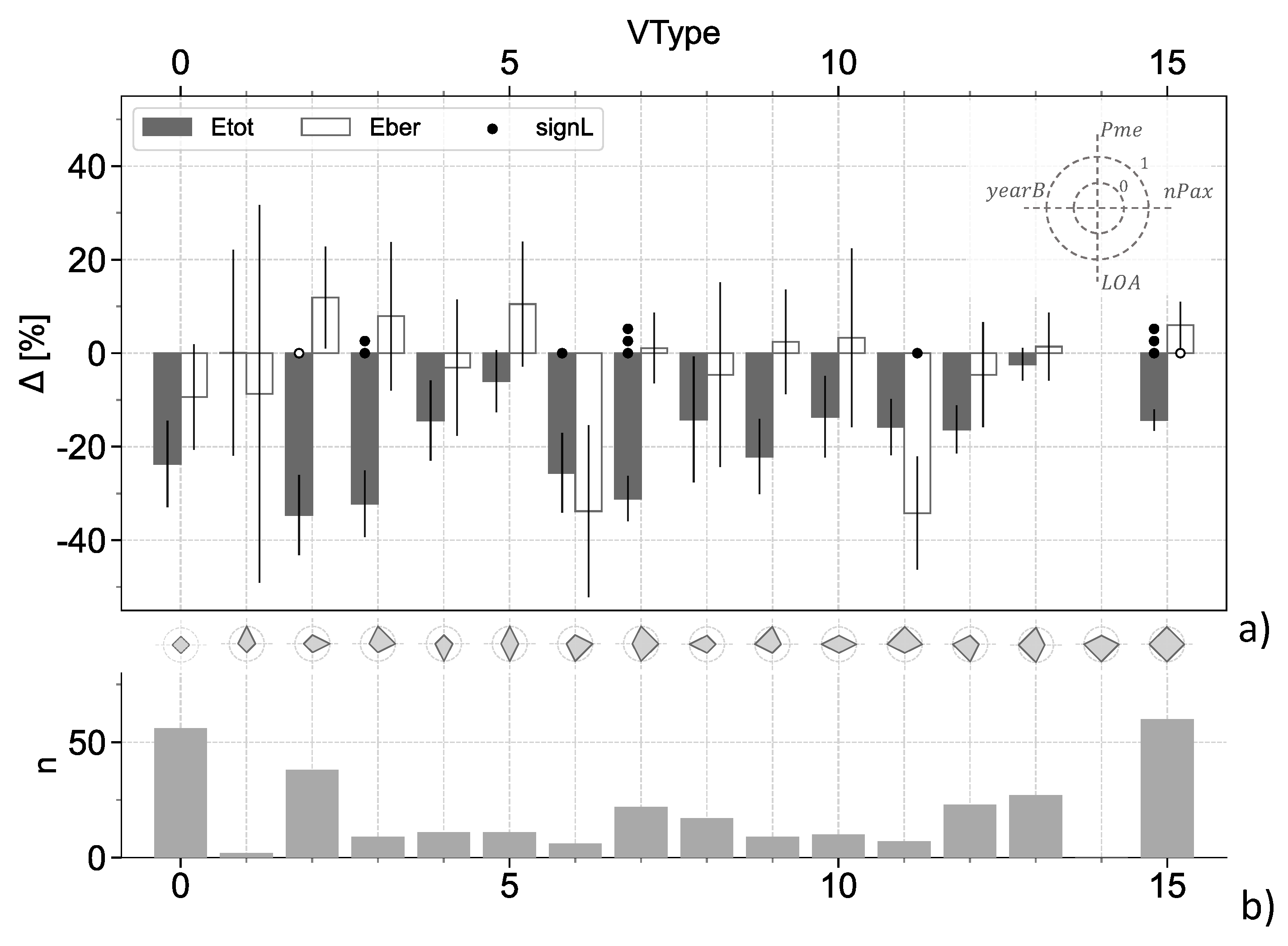
- Did the heterogeneity of the ferry fleet influence the outcome and how?
- Q2.
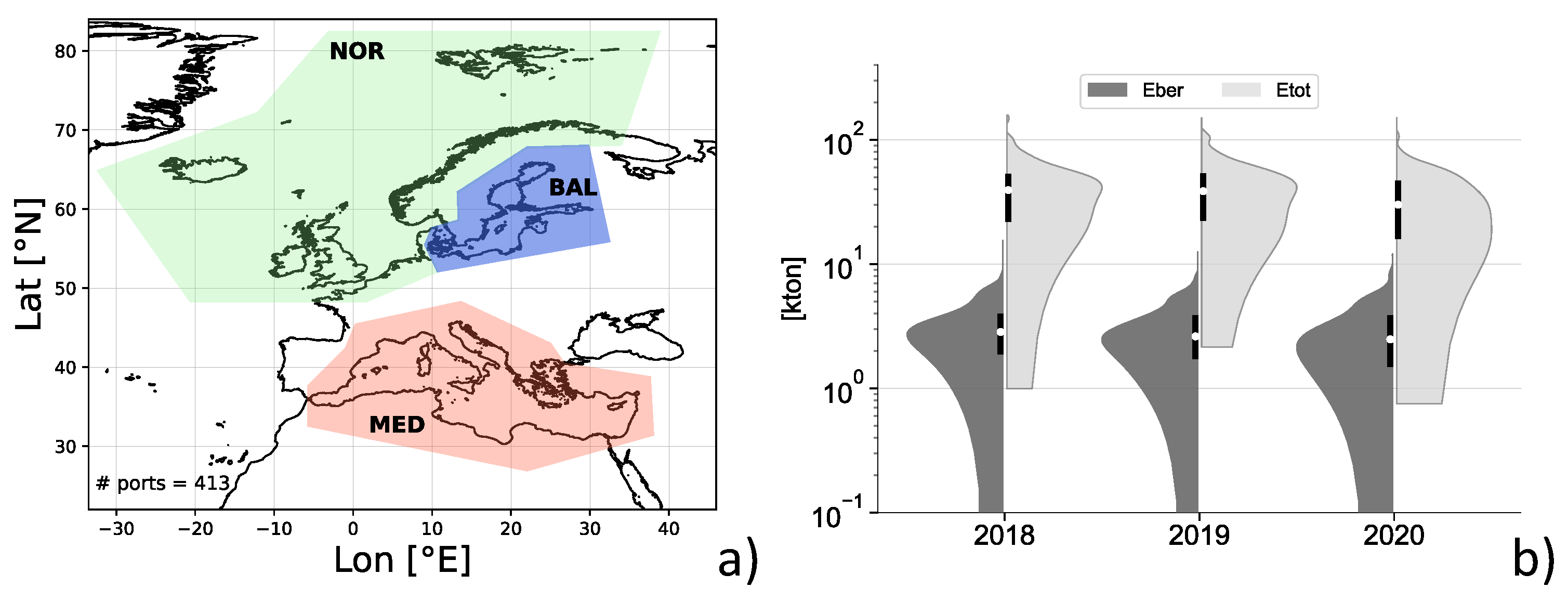
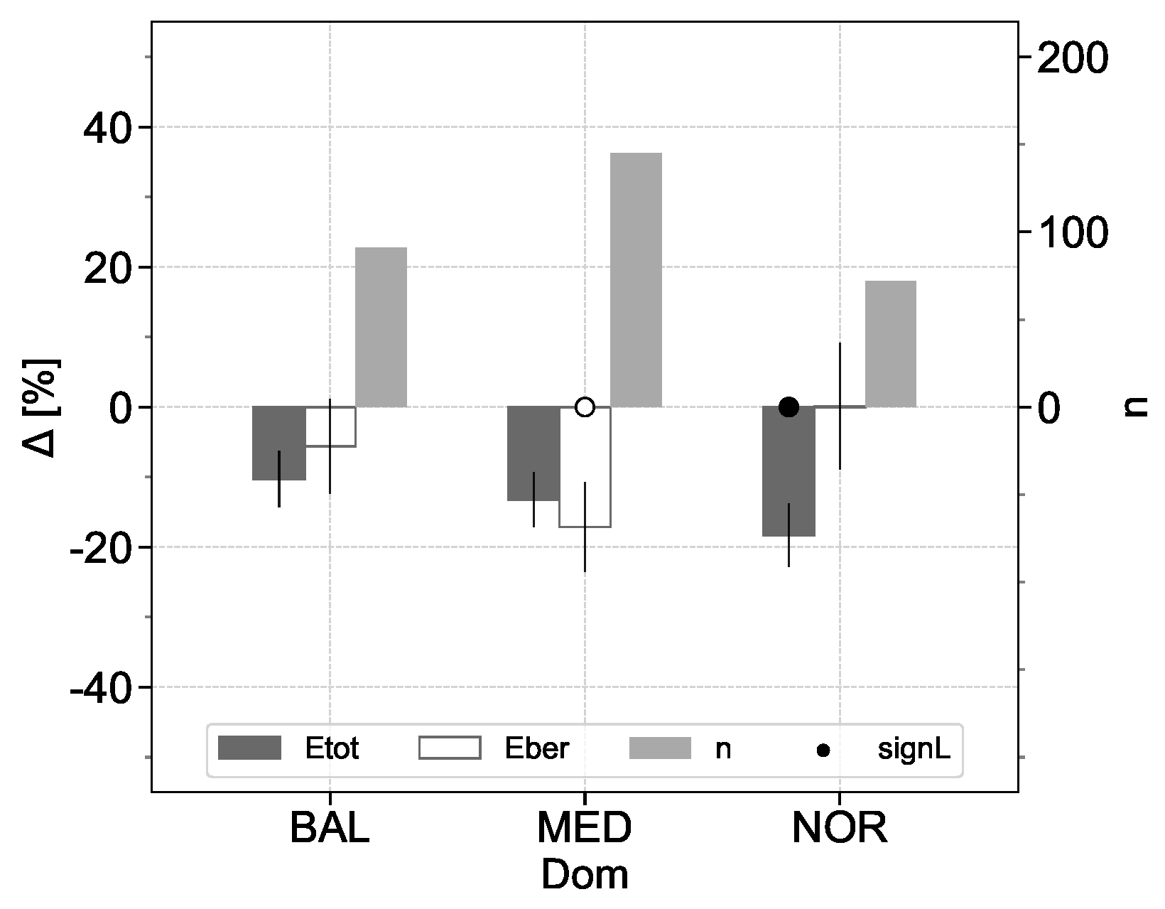
- Was there any specific geographical pattern across the European sea basins?
- Q3.
- Was the change related to the way the vessels were operated, in particular their number of port calls?
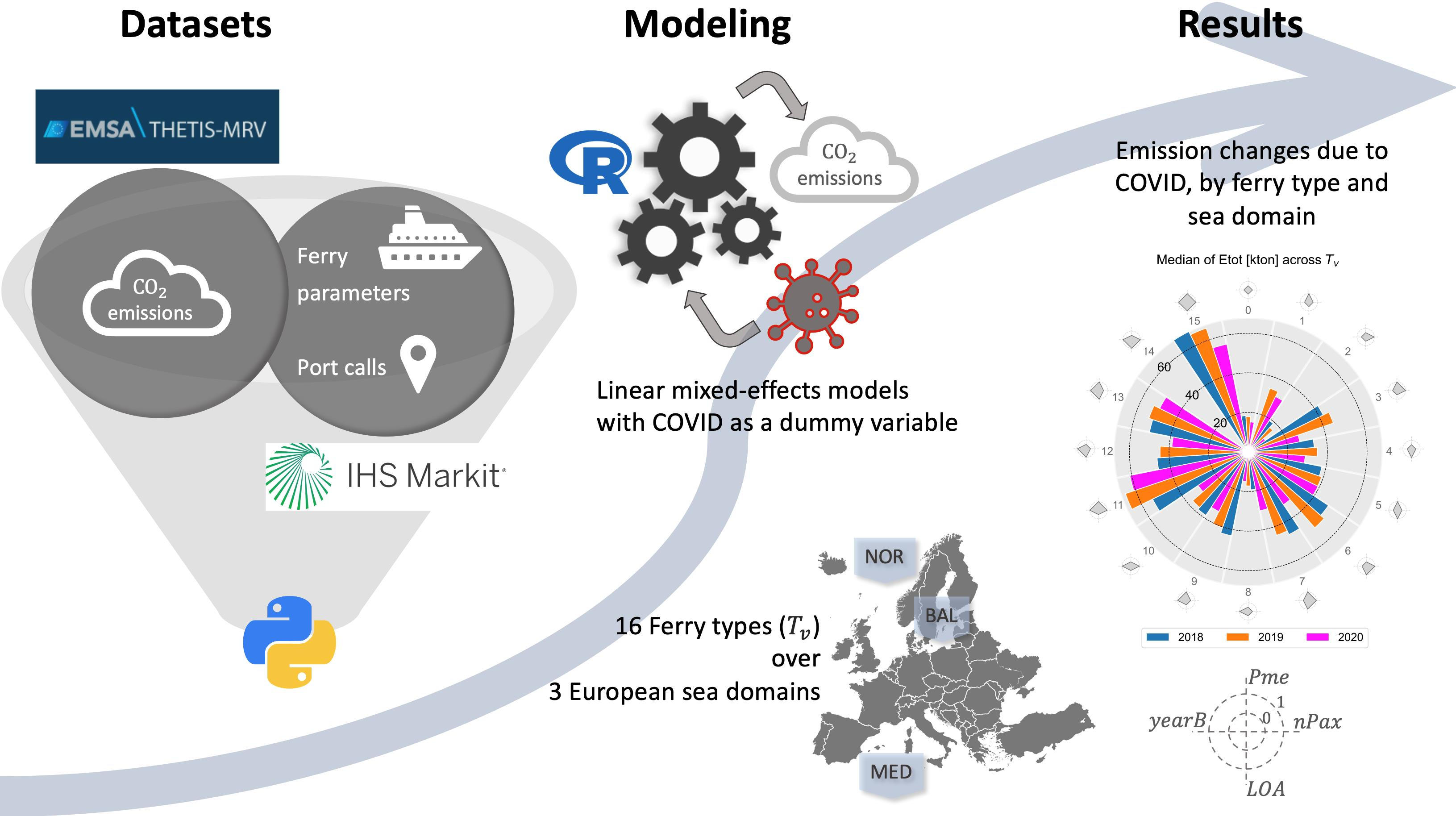
3. Data and Preprocessing
3.1. Datasets and Variables
3.2. Preprocessing of THETIS
3.3. Preprocessing of IHS
4. Preliminary Analysis
5. Methods
6. Results
6.1. Selected Model
6.2. Research Questions Answered
6.2.1. Role of Vessel Type (Q1)
6.2.2. Role of Sea Basin (Q2)
6.2.3. Role of Port Calls (Q3)
7. Discussion
7.1. Data Availability
7.2. Emissions at Berth
8. Conclusions
Supplementary Materials
Author Contributions
Funding
Data Availability Statement
Conflicts of Interest
Abbreviations
| AIC | Akaike’s information criterium |
| AIS | Automatic Identification System |
| CO | carbon dioxide |
| COVID | coronavirus disease of 2019 |
| EMSA | European Maritime Safety Agency |
| EU | European Union |
| EU-MRV | EU Monitoring Reporting Verification |
| GHG | greenhouse gas(es) |
| GT | Gross Tonnes (a vessel’s size metric) |
| HSC | high speed craft |
| IMO | International Maritime Organization |
| LME | linear-mixed effects |
| RMSEvC | conditional root mean square error of the validation set |
| Ro-Pax | roll-on/roll-off passenger ship |
| SE | standard error |
Appendix A
Appendix A.1. Input Dataset
Appendix A.2. Source Code
References
- Pan, Y.; Darzi, A.; Kabiri, A.; Zhao, G.; Luo, W.; Xiong, C.; Zhang, L. Quantifying human mobility behaviour changes during the COVID-19 outbreak in the United States. Sci. Rep. 2020, 10, 20742. [Google Scholar] [CrossRef] [PubMed]
- Le Quéré, C.; Peters, G.P.; Friedlingstein, P.; Andrew, R.M.; Canadell, J.G.; Davis, S.J.; Jackson, R.B.; Jones, M.W. Fossil CO2 emissions in the post-COVID-19 era. Nat. Clim. Chang. 2021, 11, 197–199. [Google Scholar] [CrossRef]
- Menut, L.; Bessagnet, B.; Siour, G.; Mailler, S.; Pennel, R.; Cholakian, A. Impact of lockdown measures to combat COVID-19 on air quality over western Europe. Sci. Total Environ. 2020, 741, 140426. [Google Scholar] [CrossRef]
- Ropkins, K.; Tate, J.E. Early observations on the impact of the COVID-19 lockdown on air quality trends across the UK. Sci. Total Environ. 2021, 754, 142374. [Google Scholar] [CrossRef]
- Guan, D.; Wang, D.; Hallegatte, S.; Davis, S.J.; Huo, J.; Li, S.; Bai, Y.; Lei, T.; Xue, Q.; Coffman, D.; et al. Global supply-chain effects of COVID-19 control measures. Nat. Hum. Behav. 2020, 4, 577–587. [Google Scholar] [CrossRef]
- Moriarty, L.F.; Plucinski, M.M.; Marston, B.J.; Kurbatova, E.V.; Knust, B.; Murray, E.L.; Pesik, N.; Rose, D.; Fitter, D.; Kobayashi, M.; et al. Public health responses to COVID-19 outbreaks on cruise ships—Worldwide, February–March 2020. Morb. Mortal. Wkly. Rep. 2020, 69, 347. [Google Scholar] [CrossRef]
- UNCTAD. COVID-19 and Maritime Transport Impact and Responses; Transport and Trade Facilitation 15; United Nations: New York, NY, USA, 2021. [Google Scholar]
- EMSA. COVID-19—Impact on Shipping; Technical Report; European Maritime Safety Agency: Lisbon, Portugal, 2021. [Google Scholar]
- EU. Regulation 2015/757 of 29 April 2015 on the Monitoring, Reporting and Verification of Carbon Dioxide Emissions from Maritime Transport, and Amending Directive 2009/16/EC; Technical Report; European Parliament and the Council: Strasbourg, France, 2015. [Google Scholar]
- Chowdhury, R.B.; Khan, A.; Mahiat, T.; Dutta, H.; Tasmeea, T.; Binth Arman, A.B.; Fardu, F.; Roy, B.B.; Hossain, M.M.; Khan, N.A.; et al. Environmental externalities of the COVID-19 lockdown: Insights for sustainability planning in the Anthropocene. Sci. Total Environ. 2021, 783, 147015. [Google Scholar] [CrossRef]
- Rutz, C.; Loretto, M.C.; Bates, A.E.; Davidson, S.C.; Duarte, C.M.; Jetz, W.; Johnson, M.; Kato, A.; Kays, R.; Mueller, T.; et al. COVID-19 lockdown allows researchers to quantify the effects of human activity on wildlife. Nat. Ecol. Evol. 2020, 4, 1156–1159. [Google Scholar] [CrossRef]
- Angrist, J.D.; Krueger, A.B. Instrumental variables and the search for identification: From supply and demand to natural experiments. J. Econ. Perspect. 2001, 15, 69–85. [Google Scholar] [CrossRef] [Green Version]
- Marzano, V.; Tocchi, D.; Fiori, C.; Tinessa, F.; Simonelli, F.; Cascetta, E. Ro-Ro/Ro-Pax maritime transport in Italy: A policy-oriented market analysis. Case Stud. Transp. Policy 2020, 8, 1201–1211. [Google Scholar] [CrossRef]
- Wergeland, T. The Blackwell Companion to Maritime Economics; Ferry Passenger Markets; Wiley-Blackwell Publishing: Oxford, UK, 2012; Chapter 9; pp. 161–183. [Google Scholar]
- March, D.; Metcalfe, K.; Tintoré, J.; Godley, B.J. Tracking the global reduction of marine traffic during the COVID-19 pandemic. Nat. Commun. 2021, 12, 2415. [Google Scholar] [CrossRef] [PubMed]
- Cacciapaglia, G.; Cot, C.; Sannino, F. Multiwave pandemic dynamics explained: How to tame the next wave of infectious diseases. Sci. Rep. 2021, 11, 6638. [Google Scholar] [CrossRef] [PubMed]
- Millefiori, L.M.; Braca, P.; Zissis, D.; Spiliopoulos, G.; Marano, S.; Willett, P.K.; Carniel, S. COVID-19 impact on global maritime mobility. Sci. Rep. 2021, 11, 18039. [Google Scholar] [CrossRef] [PubMed]
- UNCTAD. Review of Maritime Transport 2021; Technical Report; United Nations: New York, NY, USA, 2021. [Google Scholar]
- Notteboom, T.; Pallis, T.; Rodrigue, J.P. Disruptions and resilience in global container shipping and ports: The COVID-19 pandemic versus the 2008–2009 financial crisis. Marit. Econ. Logist. 2021, 23, 179–210. [Google Scholar] [CrossRef]
- Durán-Grados, V.; Amado-Sánchez, Y.; Calderay-Cayetano, F.; Rodríguez-Moreno, R.; Pájaro-Velázquez, E.; Ramírez-Sánchez, A.; Sousa, S.I.V.; Nunes, R.A.O.; Alvim-Ferraz, M.C.M.; Moreno-Gutiérrez, J. Calculating a Drop in Carbon Emissions in the Strait of Gibraltar (Spain) from Domestic Shipping Traffic Caused by the COVID-19 Crisis. Sustainability 2020, 12, 10368. [Google Scholar] [CrossRef]
- Ju, Y.; Hargreaves, C.A. The impact of shipping CO2 emissions from marine traffic in Western Singapore Straits during COVID-19. Sci. Total Environ. 2021, 789, 148063. [Google Scholar] [CrossRef]
- Wang, C.; Li, G.; Han, P.; Osen, O.; Zhang, H. Impacts of COVID-19 on Ship Behaviours in Port Area: An AIS Data-Based Pattern Recognition Approach. IEEE Trans. Intell. Transp. Syst. 2022, 1–12. [Google Scholar] [CrossRef]
- Grythe, H.; Lopez-Aparicio, S. The who, why and where of Norway’s CO2 emissions from tourist travel. Environ. Adv. 2021, 5, 100104. [Google Scholar] [CrossRef]
- Chen, Q.; Ge, Y.E.; yip Lau, Y.; Dulebenets, M.A.; Sun, X.; Kawasaki, T.; Mellalou, A.; Tao, X. Effects of COVID-19 on passenger shipping activities and emissions: Empirical analysis of passenger ships in Danish waters. Marit. Policy Manag. 2022, 1–21. [Google Scholar] [CrossRef]
- Liu, Z.; Ciais, P.; Deng, Z.; Lei, R.; Davis, S.J.; Feng, S.; Zheng, B.; Cui, D.; Dou, X.; Zhu, B.; et al. Near-real-time monitoring of global CO2 emissions reveals the effects of the COVID-19 pandemic. Nat. Commun. 2020, 11, 5172. [Google Scholar] [CrossRef]
- Friedlingstein, P.; Jones, M.W.; O’Sullivan, M.; Andrew, R.M.; Bakker, D.C.E.; Hauck, J.; Le Quéré, C.; Peters, G.P.; Peters, W.; Pongratz, J.; et al. Global Carbon Budget 2021. Earth Syst. Sci. Data Discuss. 2021, 2021, 1–191. [Google Scholar] [CrossRef]
- Jackson, R.; Friedlingstein, P.; Le Quéré, C.; Abernethy, S.; Andrew, R.; Canadell, J.; Ciais, P.; Davis, S.; Deng, Z.; Liu, Z.; et al. Global fossil carbon emissions rebound near pre-COVID-19 levels. Environ. Res. Lett. 2022, 17, 031001. [Google Scholar] [CrossRef]
- IPCC. Sixth Assessment Report; Technical Report; IPCC: Geneva, Switzerland, 2021. [Google Scholar]
- Rehmatulla, N.; Calleya, J.; Smith, T. The implementation of technical energy efficiency and CO2 emission reduction measures in shipping. Ocean Eng. 2017, 139, 184–197. [Google Scholar] [CrossRef]
- Zis, T.P.; Psaraftis, H.N.; Ding, L. Ship weather routing: A taxonomy and survey. Ocean Eng. 2020, 213, 107697. [Google Scholar] [CrossRef]
- Lagouvardou, S.; Psaraftis, H.N.; Zis, T. A Literature Survey on Market-Based Measures for the Decarbonization of Shipping. Sustainability 2020, 12, 3953. [Google Scholar] [CrossRef]
- Lindstad, E.; Lagemann, B.; Rialland, A.; Gamlem, G.M.; Valland, A. Reduction of maritime GHG emissions and the potential role of E-fuels. Transp. Res. Part D Transp. Environ. 2021, 101, 103075. [Google Scholar] [CrossRef]
- IMO. MEPC.304(72) Initial IMO Strategy on Reduction of GHG Emissions from Ships; Technical Report Annex 11; International Maritime Organization: London, UK, 2018. [Google Scholar]
- IMO. MEPC 76/WP1/Rev.1 Draft Report of The Marine Environment Protection Committee On Its Seventy-Sixth Session; Technical Report; International Maritime Organization: London, UK, 2021. [Google Scholar]
- Panagakos, G.; Pessôa, T.d.S.; Dessypris, N.; Barfod, M.B.; Psaraftis, H.N. Monitoring the carbon footprint of dry bulk shipping in the EU: An early assessment of the MRV regulation. Sustainability 2019, 11, 5133. [Google Scholar] [CrossRef] [Green Version]
- Baltagi, B.H. Panel data methods. In Handbook of Applied Economic Statistics; CRC Press: Boca Raton, FL, USA, 1998; pp. 311–323. [Google Scholar]
- Fahrmeir, L.; Kneib, T.; Lang, S.; Marx, B. Regression models. In Regression; Springer: Berlin/Heidelberg, Germany, 2013; pp. 21–72. [Google Scholar]
- Zuur, A.; Ieno, E.N.; Walker, N.; Saveliev, A.A.; Smith, G.M. Mixed Effects Models and Extensions in Ecology with R; Springer Science & Business Media: Berlin/Heidelberg, Germany, 2009. [Google Scholar]
- Merkert, R.; Mulley, C. Chapter 18 - Panel Data in Transportation Research. In Panel Data Econometrics; Tsionas, M., Ed.; Academic Press: Cambridge, MA, USA, 2019; pp. 583–608. [Google Scholar]
- Lv, T.; Wu, X. Using Panel Data to Evaluate the Factors Affecting Transport Energy Consumption in China’s Three Regions. Int. J. Environ. Res. Public Health 2019, 16, 555. [Google Scholar] [CrossRef] [Green Version]
- Xu, L.; Shi, J.; Chen, J.; Li, L. Estimating the effect of COVID-19 epidemic on shipping trade: An empirical analysis using panel data. Mar. Policy 2021, 133, 104768. [Google Scholar] [CrossRef]
- Tianming, G.; Erokhin, V.; Arskiy, A.; Khudzhatov, M. Has the COVID-19 Pandemic Affected Maritime Connectivity? An Estimation for China and the Polar Silk Road Countries. Sustainability 2021, 13, 3521. [Google Scholar] [CrossRef]
- Poulsen, R.T.; Viktorelius, M.; Varvne, H.; Rasmussen, H.B.; von Knorring, H. Energy efficiency in ship operations—Exploring voyage decisions and decision-makers. Transp. Res. Part D Transp. Environ. 2022, 102, 103120. [Google Scholar] [CrossRef]
- Mannarini, G.; Carelli, L. VISIR-1.b: Ocean surface gravity waves and currents for energy-efficient navigation. Geosci. Model Dev. 2019, 12, 3449–3480. [Google Scholar] [CrossRef] [Green Version]
- Chu-Van, T.; Ristovski, Z.; Pourkhesalian, A.M.; Rainey, T.; Garaniya, V.; Abbassi, R.; Jahangiri, S.; Enshaei, H.; Kam, U.S.; Kimball, R.; et al. On-board measurements of particle and gaseous emissions from a large cargo vessel at different operating conditions. Environ. Pollut. 2018, 237, 832–841. [Google Scholar] [CrossRef] [PubMed] [Green Version]
- INTERFERRY. MEPC 76/7/14 Reduction of GHG Emissions from Ships; Technical Report; International Maritime Organization: London, UK, 2021. [Google Scholar]
- Grigoropoulos, G. Recent Advances in the Hydrodynamic Design of Fast Monohulls. Ship Technol. Res. 2005, 52, 14–33. [Google Scholar] [CrossRef]
- Mannarini, G.; Carelli, L.; Orović, J.; Martinkus, C.P.; Coppini, G. toward Least-CO2 Ferry Routes in the Adriatic Sea. J. Mar. Sci. Eng. 2021, 9, 115. [Google Scholar] [CrossRef]
- James, G.; Witten, D.; Hastie, T.; Tibshirani, R. An Introduction to Statistical Learning; Springer: Berlin/Heidelberg, Germany, 2013. [Google Scholar]
- Beven, K. Validation and Equifinality. In Computer Simulation Validation; Springer: Berlin/Heidelberg, Germany, 2019; pp. 791–809. [Google Scholar]
- Mannarini, G.; Carelli, L.; Salhi, A. EU-MRV: An analysis of 2018’s Ro-Pax CO2 data. In Proceedings of the 21st IEEE International Conference on Mobile Data Management (MDM), Versailles, France, 30 June–3 July 2020; pp. 287–292. [Google Scholar]
- Mocerino, L.; Quaranta, F. How emissions from cruise ships in the port of Naples changed in the COVID-19 lock down period. Proc. Inst. Mech. Eng. Part M J. Eng. Marit. Environ. 2021, 236, 125–130. [Google Scholar] [CrossRef]
- Capezza, C.; Centofanti, F.; Lepore, A.; Menafoglio, A.; Palumbo, B.; Vantini, S. Functional regression control chart for monitoring ship CO2 emissions. Qual. Reliab. Eng. Int. 2021. [Google Scholar] [CrossRef]
- Capezza, C.; Lepore, A.; Menafoglio, A.; Palumbo, B.; Vantini, S. Control charts for monitoring ship operating conditions and CO2 emissions based on scalar-on-function regression. Appl. Stoch. Model. Bus. Ind. 2020, 36, 477–500. [Google Scholar] [CrossRef]
- Gavalas, D.; Syriopoulos, T.; Tsatsaronis, M. COVID–19 impact on the shipping industry: An event study approach. Transp. Policy 2022, 116, 157–164. [Google Scholar] [CrossRef]
- Jolly, E. Pymer4: Connecting R and Python for linear mixed modeling. J. Open Source Softw. 2018, 3, 862. [Google Scholar] [CrossRef]


| Dataset | Source Variable | Acronym | Description | Units/Type |
|---|---|---|---|---|
| THETIS | IMO number | IMOn | Vessel unique identifier | - |
| Total emissions | Etot | Per-ship total emissions | [ton] | |
| CO emissions which occurred within ports under a MS jurisdiction at berth | Eber | Per-ship emissions at berth | [ton] | |
| IHS | Speedservice | maxV | Service speed | [kts] |
| ConsumptionValue1 | FuelC | Fuel consumption rate | [ton/h] | |
| TotalKilowattsofMainEngines | Pme | Total power of main engines | [kW] | |
| TotalPowerOfAuxiliaryEngines | Paux | Power of auxiliary engines | [kW] | |
| PassengerCapacity | nPax | Passenger carrying capacity | - | |
| LengthOverallLOA | LOA | Length over all | [m] | |
| YearOfBuild | yearB | Year of building | - | |
| IHS-derived | several | VType | Vessel type of Equation (2) | [categorical] |
| Port Latitude/Longitude Decimal | Dom | Sea basin (BAL, MED, NOR) | [categorical] | |
| Call ID | nCalls | Per-ship number of port calls | - | |
| - | COVID | Dummy variable for year 2020 | [categorical] |
| Subset | All | Non-HSC | |||||||||
|---|---|---|---|---|---|---|---|---|---|---|---|
| Etot | Eber | Etot | Eber | nCalls | Pruned | ||||||
| 2018-v217 | 142.19 | 8.71 | 12,059 | 13.03 | 0.96 | 231,332 | 321 | 4 | |||
| 2019-v191 | 146.3 | 9.21 | 12,336 | 13.53 | 0.5 | 1.01 | 0.05 | 265,193 | 33,861 | 345 | 8 |
| 2020-v62 | 125.83 | 8.09 | 11,676 | 10.95 | −2.58 | 0.94 | −0.07 | 230,626 | −34,567 | 325 | 4 |
| k | Units | ||
|---|---|---|---|
| 0 | Pme | 21,600 | kW |
| 1 | nPax | 1250 | - |
| 2 | LOA | 174 | m |
| 3 | yearB | 1999 | - |
| Etot | nCalls | Eber | |||||||
|---|---|---|---|---|---|---|---|---|---|
| [ton] | [%] | SignL | [# per Ship] | [%] | SignL | [ton] | [%] | SignL | |
| 2018 | 37,482 | 467 | 2779 | ||||||
| 2019 | 37,432 | 475 | 2621 | ||||||
| 2020 | 30,182 | 402 | 2474 | ||||||
| 2019 vs. 2018 | −480 | −1.7 | ∘ | 0 | 0 | −30 | −1.4 | ||
| 2020 vs. 2019 | −4418 | −15.4 | −33 | −6.8 | −104 | −5.9 | ∘ | ||
| Symbol | p | Predicate | |
|---|---|---|---|
| bi | uni | ||
| ∘ | 0.08 | 0.04 | Nearly significant |
| • | 0.05 | 0.0025 | Slightly significant |
| 0.01 | 0.005 | Significant | |
| 0.001 | 0.0005 | Highly significant | |
| Etot | Eber | ||||||||||
| [t] | SE [t] | signL | [t] | SE [t] | signL | ||||||
| −4169 | 1620 | • | COVID | 308 | −180 | 216 | |||||
| COVID : VType | |||||||||||
| [t] | SE [t] | signL | VType | Pme | nPax | LOA | yearB | [t] | SE [t] | signL | |
| - | - | - | 0 | - | - | - | - | 56 | - | - | - |
| 4214 | 7526 | 1 | > | - | - | - | 2 | −37.4 | 1,010 | ||
| −3514 | 1955 | ∘ | 2 | - | > | - | - | 38 | 458.2 | 261 | |
| −9698 | 3249 | 3 | > | > | - | - | 9 | 382.7 | 433 | ||
| −552 | 3057 | 4 | - | - | > | - | 11 | 97.9 | 409 | ||
| 1568 | 2976 | 5 | > | - | > | - | 11 | 481.3 | 399 | ||
| −8165 | 4139 | • | 6 | - | > | > | - | 6 | −827.4 | 553 | |
| −9602 | 2296 | 7 | > | > | > | - | 22 | 220.7 | 308 | ||
| 1450 | 2565 | 8 | - | - | - | > | 17 | 98.4 | 343 | ||
| −5116 | 3413 | 9 | > | - | - | > | 9 | 275.1 | 457 | ||
| −919 | 3210 | 10 | - | > | - | > | 10 | 255.5 | 429 | ||
| −5513 | 3624 | 11 | > | > | - | > | 7 | −1199 | 484 | • | |
| −2956 | 2342 | 12 | - | - | > | > | 23 | 55.3 | 313 | ||
| 2843 | 2147 | 13 | > | - | > | > | 27 | 228.3 | 288 | ||
| 14 | - | > | > | > | 0 | ||||||
| −6143 | 1719 | 15 | > | > | > | > | 60 | 447.5 | 230 | ∘ | |
| Total | 308 | ||||||||||
| [t] | SE [t] | signL | COVID : Dom | [t] | SE [t] | signL | |||||
| - | - | - | BAL | 91 | - | - | - | ||||
| −666 | 1327 | MED | 145 | −332 | 178 | ∘ | |||||
| −3514 | 1590 | • | NOR | 72 | 181 | 212 | |||||
| [t] | SE [t] | signL | [t] | SE [t] | signL | ||||||
| 1.1 | 0.6 | COVID : nCalls | 308 | 0 | 0.1 | ||||||
| Etot | Eber | ||||
| units | ref. | COVID | ref. | COVID | |
| nsamples | - | 648 | 308 | 648 | 308 |
| std | 5667 | 6672 | 793 | 896 | |
| skewness | - | 0.2 | −0.3 | 1 | 0.7 |
| kurtosis | - | 5.0 | 2.0 | 6.2 | 2.1 |
Publisher’s Note: MDPI stays neutral with regard to jurisdictional claims in published maps and institutional affiliations. |
© 2022 by the authors. Licensee MDPI, Basel, Switzerland. This article is an open access article distributed under the terms and conditions of the Creative Commons Attribution (CC BY) license (https://creativecommons.org/licenses/by/4.0/).
Share and Cite
Mannarini, G.; Salinas, M.L.; Carelli, L.; Fassò, A. How COVID-19 Affected GHG Emissions of Ferries in Europe. Sustainability 2022, 14, 5287. https://doi.org/10.3390/su14095287
Mannarini G, Salinas ML, Carelli L, Fassò A. How COVID-19 Affected GHG Emissions of Ferries in Europe. Sustainability. 2022; 14(9):5287. https://doi.org/10.3390/su14095287
Chicago/Turabian StyleMannarini, Gianandrea, Mario Leonardo Salinas, Lorenzo Carelli, and Alessandro Fassò. 2022. "How COVID-19 Affected GHG Emissions of Ferries in Europe" Sustainability 14, no. 9: 5287. https://doi.org/10.3390/su14095287
APA StyleMannarini, G., Salinas, M. L., Carelli, L., & Fassò, A. (2022). How COVID-19 Affected GHG Emissions of Ferries in Europe. Sustainability, 14(9), 5287. https://doi.org/10.3390/su14095287