Using a Choice Experiment to Understand Preferences for Disaster Risk Reduction with Uncertainty: A Case Study in Japan

Abstract

With the increase in disasters due to climate change, there has been a growing interest in green infrastructures that utilize nature for disaster risk reduction (DRR). However, green infrastructures cannot completely protect against hazards. Therefore, this study investigates the public preference in Japan for DRR and its uncertainty using a survey-based choice experiment. The results showed that benefits were obtained from the increase in “success probability”, “reduction in human damage”, “reduction in property damage”, and “reduction in indirect damage”; however, the benefits obtained from additional improvements diminished. Moreover, the results of our analyses revealed that preferences for DRR and its uncertainty were heterogeneous among respondents, and the population segment that includes more women, older people, and more people who live in areas that may be directly affected by floods had higher ratings for “success probability” and relatively slightly lower ratings for “reduction in indirect damage”.

1. Introduction

1.1. Background

Due to climate change, the occurrence of disasters has increased significantly, thus making the development of infrastructure for disaster prevention and mitigation extremely important [1,2]. In particular, green infrastructures, which are sometimes referred to as nature-based solutions and utilize the functions of nature to cope with disasters, have been attracting considerable attention [3,4]. Green infrastructures not only have a smaller impact on ecosystems and landscapes than artificial infrastructures (hereafter, gray infrastructures), such as dams and seawalls, but are often less expensive to build and maintain [5,6,7]. In countries with aging populations, including Japan, it is expected that the infrastructure maintenance costs will become a major burden in many areas owing to the worsening financial situation caused by a declining population, highlighting the need to control these costs. For disaster risk reduction (DRR), ecosystem-based disaster risk reduction (Eco-DRR), which utilizes green infrastructures, can be a cost-effective method and is expected to expand [8,9,10,11,12,13].

Nevertheless, green infrastructures cannot completely protect against hazards [14]. Thus, not always achieving the targeted DRR, that is, uncertainty in DRR, is one of the characteristics of green infrastructures as opposed to gray infrastructures, which are designed based on accumulated knowledge that achieves targeted effects with a high degree of certainty [15]. If citizens tend to not tolerate this uncertainty in DRR, it will be difficult for green infrastructures to proliferate. Therefore, understanding public preferences with respect to uncertainty in DRR is important for the diffusion of green infrastructures.

1.2. Green Infrastructures in the United States (U.S.), Europe, and Japan

As “green infrastructures” is a relatively new concept, it has no worldwide consensus definition [16].

In the U.S., green infrastructures are being used for stormwater management. The U.S. Environmental Protection Agency (2008) states that “Green infrastructure is an approach to wet weather management that uses soils and vegetation to utilize, enhance and/or mimic the natural hydrological cycle processes of infiltration, evapotranspiration, and reuse.” [17] Today, a variety of green infrastructures are used, including green roofs, rain gardens, and permeable pavements. Portland, Oregon, is a world-renowned green infrastructure-advanced city. In Portland, heavy rains often caused internal flooding; therefore, green infrastructures were installed in residential neighborhoods as countermeasures. As a result, green infrastructures have not only achieved their original purpose but have also brought about diverse benefits, such as improved air quality, improved health through the promotion of physical activity, and increased mental health through stress reduction [18].

Europe emphasizes the conservation and utilization of broader ecological networks. In Europe, the European Commission adopted a strategy in 2013 to promote the use of green infrastructures. Green infrastructure is defined as a strategically planned network of natural and semi-natural areas with other environmental features designed and managed to deliver a wide range of ecosystem services [19]. Since then, European countries have been promoting green infrastructures.

In Japan, green infrastructures have recently been incorporated into various administrative plans, such as the National Spatial Strategy (National Plan) and are being promoted. This plan describes green infrastructure as a way to utilize the diverse functions of the natural environment, in both hard and soft aspects of social capital development and land utilization, to create sustainable and attractive national lands and regions [20]. There are also examples of local governments undertaking their own green infrastructure initiatives. For example, Setagaya City, Tokyo, has incorporated “promotion of green infrastructure” in its action plan for heavy rainfall countermeasures [21]. Numerous initiatives, including those that are not called green infrastructure or Eco-DRR, are underway. For example, various disaster countermeasures, such as flood mitigation through the water storage function of rice paddies, mitigation of landslides by planting trees on mountain slopes, coastal forests to reduce tsunami damage, flood control using retarding basins, and flood prevention by preserving wetlands, are being implemented [8].

1.3. Literature Review

There has been exponential growth in the number of studies on green infrastructures [22]. Previous studies that also used the choice experiment (CE), are as follows:

Veronesi et al. (2014) conducted a choice experiment in Switzerland and found that more than 70% of the respondents were willing to pay a higher tax to reduce the risk of combined sewer overflows (CSOs) in rivers and lakes, and that climate change perception affected their willingness to pay (WTP) [23].

Brouwer et al. (2016) conducted an identical choice experiment on river restoration in Austria, Hungary, and Romania and showed that estimated benefits were transferable between Hungary and Romania, however, not between Austria and Hungary and Austria and Romania [24]. They also found distance decay effects for water quality improvements in Austria and Romania, and for flood risk reduction in Austria.

Brent et al. (2017) estimated the willingness of the residential homeowners in Melbourne and Sydney, Australia, to pay for the ecosystem services provided by green infrastructures for stormwater management and showed that respondents were willing to pay for the prevention of flash flooding [25]. This study also showed that benefits from stormwater management via green infrastructures were transferable to different locations.

Valasiuk et al. (2018) employed a choice experiment to investigate citizens’ preferences for forest landscape restoration in a transboundary region in Sweden and Norway and showed that just over half of the sample were willing to pay for forest landscape restoration in both countries [26].

Meng and Hsu (2019) conducted a choice experiment with officials in water utilities and agencies in the U.S. and showed that respondents were willing to invest more in smart green infrastructures if the long-term costs associated with construction, maintenance, and labor could be reduced [27]. They also revealed that agencies with large service areas or those that utilized green infrastructures in the past, were more likely to utilize the smart green infrastructures.

Shr et al. (2019) conducted a choice experiment using a split sample methodology on the landscape attributes of green infrastructures in the U.S. and revealed the influence of images on preferences [28].

Pienaar et al. (2019) implemented a choice experiment on the conservation program and ecosystem services provided for residents of Palm Beach County, Florida, U.S., and showed that residents were willing to pay for flood risk reduction, and there was heterogeneity in preference for habitat conservation and ecosystem services [29].

Ando et al. (2020) conducted a choice experiment to estimate the benefits from stormwater management utilizing green infrastructures in Chicago, Illinois, and Portland in the U.S. [30]. In addition to WTP, this study assessed the benefit through time spent volunteering and found that volunteering produces positive utility.

Deely and Hynes (2020) carried out a split-sample choice experiment for the residents of the Carlingford Lough catchment in Ireland to clarify whether gray or green infrastructures are preferred by them and showed that the average respondent prefers green infrastructures to gray infrastructures [31].

Wieczerak et al. (2022) used a choice experiment to examine public preferences for green infrastructure improvements in Northern New Jersey, U.S., and revealed that residents have a relatively large WTP for improved air quality, increased water supply, and closer proximity [32].

Thus, economic valuation research on green infrastructures is increasing; however, because it is a relatively new topic, some aspects are yet to be fully studied. One of these concerns the citizens’ preferences for uncertainty in the DRR. In addition, although green infrastructures are characterized by their multifunctionality and can be used for purposes other than disaster prevention, little research has been conducted on the citizens’ preferences regarding other uses of green infrastructures. Moreover, preferences for DRR and its uncertainty may vary depending on individual socioeconomic characteristics and the likelihood of being affected by a disaster. The heterogeneity of such preferences has not been sufficiently studied.

1.4. Purpose of the Study

To fill these gaps in the extant literature, using flood control as a case study, we conducted a questionnaire survey in Japan, to investigate the public preferences for DRR and its uncertainty as well as the utilization of DRR infrastructures for other purposes. The specific research questions for this study are as follows:

• How do citizens evaluate the uncertainty in DRR?
• How much importance do citizens attach to the reduction in human, property, and indirect damage?
• When there is no flooding, for what other purposes do citizens want retarding basins and dams to be used, other than for flood control?
• How much is the citizens’ marginal willingness to pay (MWTP) for each of the following: reduction in the DRR uncertainty, reduction in human damage, reduction in property damage, reduction in indirect damage, and use of DRR infrastructure for purposes other than disaster reduction?
• Are preferences for flood control homogeneous or heterogeneous among citizens?
• If preferences for flood control are heterogeneous among citizens, what are the distinct preferences?

This study explores the answers to these research questions using a CE, one of the typical environmental valuation methods [33]. CE is a method of evaluating the value of each of the attributes that make up an alternative based on people’s choice. Using CE, it is possible to economically assess the value of the reduction in uncertainty and the improvement of various disaster mitigation effects. This facilitates evaluating the benefits of developing green infrastructures, which, in turn, enable the conduct of a cost-benefit analysis of green infrastructure development. In addition, by conducting a cost-benefit analysis of green and gray infrastructures, we can compare the two in terms of cost-effectiveness. Such results can be an important factor in deciding which approach to adopt (Ganderton (2005), Mechler (2005), and Benson and Twigg (2007) provide comprehensive explanations of the cost-benefit analysis for DRR infrastructures in their studies [34,35,36]. There are also numerous cost-benefit analysis studies and reviews for DRR infrastructures worldwide (e.g., [37,38,39,40,41,42])). In addition, in the analysis, we use estimation methods, such as the random parameter logit (RPL) model and latent class model (LCM), which allow us to understand the heterogeneity in preferences. This establishes the proportions of people with specific preferences. Such information is also useful when considering consensus building over green infrastructures [43].

2. Materials and Methods

2.1. Outline of the Survey

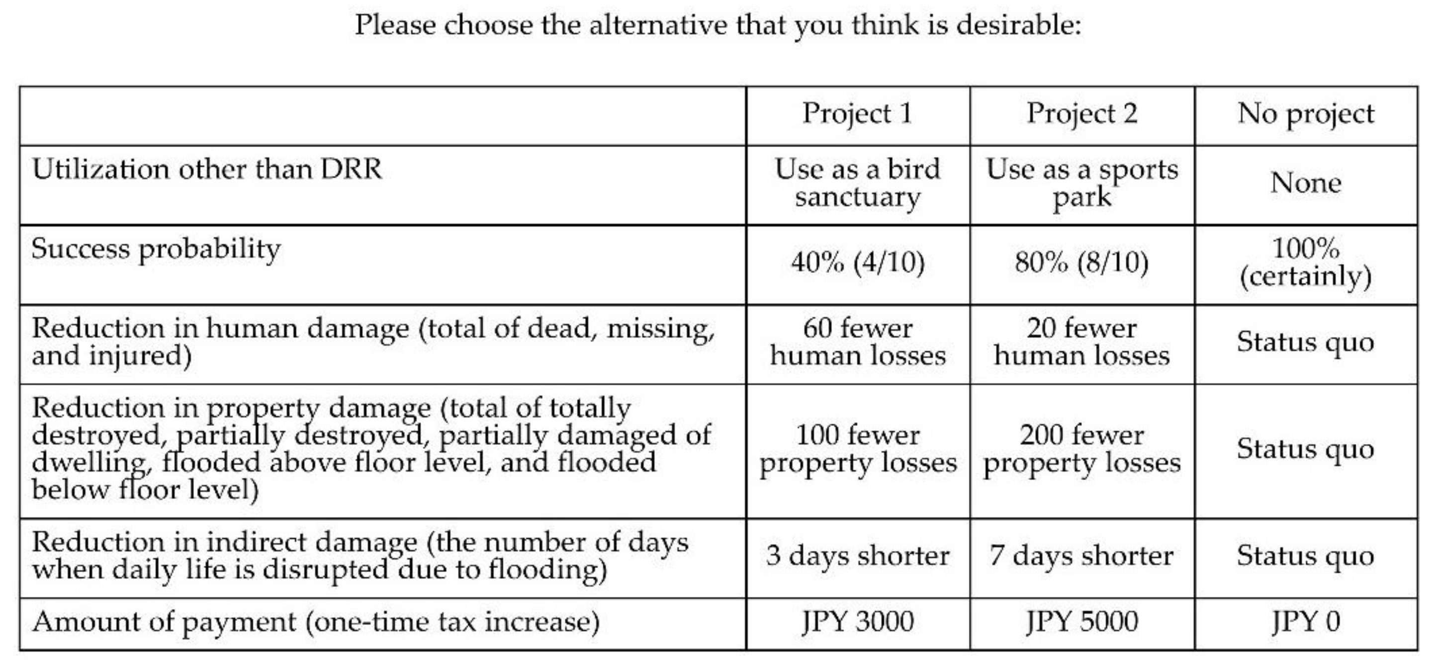
In March 2019, we conducted a web-based public survey throughout Japan. The survey participants were men and women—aged between 20 and 69 years—registered as monitors with a research company. Further, we divided the whole country into six blocks (Hokkaido and Tohoku, Kanto, Chubu, Kinki, Chugoku and Shikoku, and Kyushu and Okinawa) considering the geographical divisions of Japan. The sample collection was coordinated to reflect the population compositions of the six blocks as closely as possible in terms of gender and age. We received responses from 5224 people.

In total, the respondents comprised 50.2% men and 49.8% women. In terms of age, 15.2% of the respondents were in their 20s, 19.4% in their 30s, 23.8% in their 40s, 19.1% in their 50s, and 22.5% in their 60s. In terms of flood risk around the residence, 18.1% of the respondents lived in a place that might be directly affected by floods, 64.3% did not live in a place that might be directly affected by floods, and 17.7% did not know the flood risk around their residence. The descriptive statistics of the respondents are shown in

Table 1. Descriptive statistics of respondents (N = 5224).

	Number of People	Ratio
Gender
Male	2623	50.2%
Female	2601	49.8%
Age
20s	794	15.2%
30s	1011	19.4%
40s	1245	23.8%
50s	997	19.1%
60s	1177	22.5%
Flood risk around the residence
Live in a place that may be directly affected by floods	943	18.1%
Do not live in a place that may be directly affected by floods	3358	64.3%
Do not know	923	17.7%

.

The data used in this study are responses to a subset of the survey consisting of 47-58 multiple-choice questions that inquired about a wide range of disaster-related topics (the number of questions varied by the respondent as follow-up questions or additional questions might be asked depending on the respondent’s answers. The questionnaire (in Japanese) is available upon request to the authors). The average response time was 10.1 min.

2.2. Survey Design

Prior to the CE questions, it was explained to the respondents that the number of floods is expected to increase and that their magnitude is likely to get larger because of climate change. Then, for the CE questions, a hypothetical scenario was explained to the respondents, in which a plan was proposed to implement flood control projects, such as building dams or retarding basins upstream, to reduce the damage of floods in the area where they live.

In this CE, it was assumed that the implementation of flood control projects could reduce the three types of damages caused by floods: human, property, and indirect damage. Human damage refers to the total number of people dead, missing, or injured; property damage is defined as the total number of houses that are totally destroyed, partially destroyed, partially damaged, flooded above floor level, or flooded below floor level; indirect damage refers to the damage caused to a wide range of areas due to power outages, water shutdowns, sewage treatment facility shutdowns, and disruption of bridges and roads. To ensure that respondents understood the types of damages before answering the CE questions, we provided an explanation for all three types of damages.

It was also assumed that flood control projects would not always work as planned. Respondents were told that the effectiveness of flood control projects is uncertain, and that in some cases, projects might be successful and reduce damage, whereas in other cases, projects might fail and be ineffective. The “success probability” represents the probability that the project would be successful and reduce the damage.

Areas in which flood control projects are implemented may be used for other purposes when there is no flooding. For example, it may be possible to use the area as a sports park, since people can enjoy boating and fishing at the dam or retarding basin, or play baseball, tennis, or jog in the vicinity. Using retarding basins for purposes other than disaster prevention when no floods are occurring are taking place in Japan. For example, the Watarase retarding basin spanning four prefectures (Tochigi, Gunma, Saitama, and Ibaraki Prefectures), is used for recreation and as a habitat for wildlife during normal times without flooding. There are also many cases where dams have been designated as bird and animal sanctuaries, such as the Kurose Dam in Ehime Prefecture and the Kitayama Dam in Saga Prefecture. “Utilization other than DRR” indicates other uses for sites where the flood control projects will be implemented.

Further, it was assumed that taxes would rise only once to secure the financial resources to implement the flood control projects. The “amount of payment (one-time tax increase)” represents the amount of money the respondent would have to pay to implement the project.

In the CE, “utilization other than DRR,” “success probability,” “reduction in human damage (total number of dead, missing, and injured humans),” “reduction in property damage (total of totally destroyed, partially destroyed, partially damaged of dwelling, flooded above floor level, and flooded below floor level),” “reduction in indirect damage (the number of days when daily life is disrupted due to flooding),” and “amount of payment (one-time tax increase)” were used as the attributes.

Table 2. Attributes and levels.

	Level 1	Level 2	Level 3	Level 4	Level 5
Utilization other than DRR	None	Use as a sports park	Use as a bird sanctuary
Success probability	20% (2/10)	40% (4/10)	60% (6/10)	80% (8/10)	100% (certainly)
Reduction in human damage (total number of dead, missing, and injured humans)	20 fewer human losses	40 fewer human losses	60 fewer human losses	80 fewer human losses	100 fewer human losses
Reduction in property damage (total of totally destroyed, partially destroyed, partially damaged of dwelling, flooded above floor level, and flooded below floor level)	50 fewer property losses	100 fewer property losses	150 fewer property losses	200 fewer property losses	250 fewer property losses
Reduction in indirect damage (the number of days when daily life is disrupted due to flooding)	1 day shorter	3 days shorter	5 days shorter	7 days shorter	10 days reduction
Amount of payment (one-time tax increase)	JPY 1000	JPY 3000	JPY 5000	JPY 10,000	JPY 30,000

Note: 1 JPY= 0.0087 USD (as of 30 January 2021).

summarizes the attributes and levels used in the CE. In the case of “utilization other than DRR,” three levels were set, while for other attributes, five levels were set.

In addition to the reduction in damage and cost, which are generally important characteristics of flood control projects, we aimed to examine respondents’ preferences for uncertainty in DRR and use for purposes other than DRR. Uncertainty in DRR exists for both green and gray infrastructures, as well as their use for purposes other than DRR, but as mentioned earlier, uncertainty in DRR tends to be greater for green infrastructures, and they are often used for purposes other than DRR. From this CE, we can understand preferences for these features that are particularly important in green infrastructures. While green infrastructure has other characteristics, such as less negative impact on the landscape, we focused on these two characteristics. This helped to make the CE questions simpler and less burdensome for respondents.

A pilot survey was conducted with 217 participants. The choice set was created by combining the levels of each attribute using an orthogonal main effect design. In the actual survey, we used D-efficiency to create a choice set [44]. The estimated values with the pilot survey data were used as prior values. For the design of the choice sets, version 1.2.1 of Ngene (ChoiceMetrics, Sydney, Australia) was used.

An example of a CE question is shown in Figure 1. In this example, Projects 1 and 2 represent two different flood control projects. If Project 1 is implemented, there is a 40% (4/10) probability that there will be 60 fewer human losses, 100 fewer property losses, and the number of days that daily life is disrupted due to flooding will be reduced by 3 days. However, there is a 60% (6/10) probability that the project will be ineffective, and that the amount of human, property, and indirect damage will remain unchanged. In addition, in Project 1, the site where the project will be implemented will be used as a bird sanctuary. To implement this project, each household must bear a cost of JPY 3000.

If Project 2 is implemented, there is an 80% (8/10) probability that 20 fewer people will be negatively impacted (e.g., injury and death), 200 fewer houses will be damaged, and the number of days in which daily life will be interrupted by flooding will be reduced by 7 days. In addition, under Project 2, the area in which the project will be implemented will be used as a sports park. To implement this project, each household must bear a cost of JPY 5000.

No project means that no measures are taken. Thus, the cost will not be borne because no measures will be implemented; however, the human, property, and indirect damage caused by the flood will not be reduced, and the area will not be used as a bird sanctuary or sports park. For all CE questions, the third alternative represents “no project”.

These questions were repeated six times per respondent, and different alternatives were presented to the respondents.

2.3. Model and Estimation Methods

In the CE, a random utility model was assumed as the utility function of the respondents. In a random utility model, the utility $U_{ni}$ obtained by individual $n$ from alternative $i$ is composed of the deterministic term $V_{ni}$ and the error term ${\epsilon }_{ni}$ as follows:

$$U_{ni}=V_{ni}+{\epsilon }_{ni}.$$

(1)

Assuming a linear function, $V_{ni}$ can be described by Equation (2):

$$\begin{array}{c}{V}_{ni}={\beta }_{1}AS{C}_3+{\beta }_{2}bir{d}_{ni}+{\beta }_{3}par{k}_{ni}+{\beta }_{4}pro{b}_{ni}\\ +{\beta }_{5}huma{n}_{ni}+{\beta }_{6}pro{p}_{ni}+{\beta }_{7}in{d}_{ni}+{\beta }_{8}ta{x}_{ni}\end{array}.$$

(2)

Here, $bir{d}_{ni}$, $par{k}_{ni}$, $pro{b}_{ni}$, $huma{n}_{ni}$, $pro{p}_{ni}$, $in{d}_{ni}$, and $ta{x}_{ni}$ are variables that represent “use as a bird sanctuary,” “use as a sports park,” “success probability,” “reduction in human damage,” “reduction in property damage,” “reduction in indirect damage,” and “amount of payment (one-time tax increase)” of alternative i, respectively. $\beta$s represents their respective parameters and$AS{C}_3$ represents the alternative specific constant for alternative 3 (No project).

We assume that an individual considers the payment amount and other attributes of each alternative and chooses the alternative under which the maximum utility can be obtained. The probability $P_{ni}$ that an individual $n$ chooses alternative $i$ from the choice set $C=\left\{1, 2,\cdots ,J\right\}$, where $J$ is 3 in this case, is equal to the probability that the utility of alternative $i$, $U_{ni}$ is larger than the utility from the other alternatives$j\left( j\ne i\right)$, $U_{nj}$, as follows:

$$\begin{gathered} P_{ni}=\mathrm{Pr}\left(U_{ni}>U_{nj} \forall j\in C, j\ne i \right) \\ \hspace{1em}\hspace{1em}\hspace{1em}\hspace{1em}\hspace{1em}\hspace{1em}=\mathrm{Pr}\left(V_{ni}-V_{nj}>{\epsilon }_{nj}-{\epsilon }_{ni} \forall j\in C, j\ne i \right). \end{gathered}$$

(3)

Assuming that the error term follows a Type I extreme value distribution (Gumbel distribution), the probability $P_{ni},$ indicating that an individual $n$ will choose alternative $i$, is expressed by the following conditional logit (CL) model [45]:

$$P_{ni}=\frac{\exp \left(\mu V_{ni}\right)}{{{\displaystyle \sum }}_{j\in C}\exp \left(\mu V_{nj}\right)}.$$

(4)

The parameters can be estimated using the maximum likelihood method. $\mu$ is a scale parameter standardized to 1.

We can calculate the MWTP for each attribute or attribute-level by employing the estimated parameters. For example, in the linear model shown in equation (2), the MWTP for the success probability, $MWT{P}_{prob}$ can be calculated as the ratio of the parameters representing marginal utility of the success probability_, ${\beta }_4$, and the marginal utility of income, $-{\beta }_8$, as follows:

$$MWT{P}_{prob}=-\frac{{\beta }_4}{{\beta }_8}.$$

(5)

In the CL, it is assumed that all respondents have homogeneous preferences. In recent years, models that relax this strict assumption and capture heterogeneity in preferences have often been used, such as the RPL model, which allows parameters to vary among individuals according to a probability distribution [46,47].

If each individual has a different preference, then the parameter for each individual can be expressed as ${\beta }_n$.

$$U_{nj}={{\beta }^{\prime }}_n{x}_{nj}+{\epsilon }_{nj}.$$

(6)

Since the parameter ${\beta }_n$ for each respondent is unobservable, we consider the integral of the CL model for its density. In RPL, following Train (2009), the probability that an individual $n$ chooses an alternative $i$ is expressed as follows [47]:

$$P_{ni}\left(\mathsf{\Omega }\right)=\int \frac{\exp \left(V_{ni}\left({\beta }_n\right)\right)}{{{\displaystyle \sum }}_{j\in C}\exp \left(V_{nj}\left({\beta }_n\right)\right)}f\left(\beta |\mathsf{\Omega }\right)d\beta .$$

(7)

However, $f\left(\beta |\mathsf{\Omega }\right)$ and $\mathsf{\Omega }$ represent the probability density function of $\beta$ and the vector of parameters for this probability density function, respectively. In the estimation, it was necessary to assume a probability distribution for $\beta$. Among the various distributions that could be assumed, a normal distribution was assumed in this study [46,47]. In addition, since the integral could not be solved algebraically, the maximum simulated likelihood was used to approximate the integral using a simulation [47].

Another representative model used to understand heterogeneity in preferences is the LCM, which classifies individuals into several groups and estimates the parameters of the utility function for each group [48,49]. The membership function, which explains the probability of belonging to each class by individual characteristics such as age and gender, is estimated to investigate the factors related to heterogeneity in preferences. Therefore, it is particularly useful to understand the factors related to preference heterogeneity.

Suppose that there are S classes in the sample and that an individual $n$ belongs to class $s=\left\{1, 2,\cdots ,S\right\}$. In this case, the probability $P_{ns}\left(i\right)$ that an individual $n$ belongs to class $s$ and chooses an alternative $i$ is expressed as follows:

$$P_{ns}\left(i\right)={{\displaystyle \sum }}_{s=1}^S\left[\frac{\exp \left(\zeta {\gamma }_s^{\prime }{z}_n\right)}{{{\displaystyle \sum }}_{s^{*}=1}^{S}exp\left(\zeta {\gamma }_{s^{*}}^{\prime }{z}_n\right)}\right]\left[\frac{\exp \left({\mu }_s{\beta }_s^{\prime }{x}_{ni}\right)}{{{\displaystyle \sum }}_{j\in C}exp\left({\mu }_s{\beta }_s^{\prime }{x}_{nj}\right)}\right].$$

(8)

The first logit model equation on the right-hand side represents the membership function that expresses the probability that an individual will be assigned to class $s$, where $z_n$ is a vector of individual characteristics, ${\gamma }_s$ is a vector of the estimated parameters, and $\xi$ represents the scale parameter of the membership function, standardized to 1. The second logit model equation on the right-hand side represents the probability that an individual $n$ belonging to class $s$ will choose an alternative $i$, where $x_{ni}$ and $x_{nj}$ are the vectors of the attributes of alternatives $i$ and $j$, respectively; ${\beta }_s$ is the vector of parameters specific to class $s$; and ${\mu }_s$ represents a scale parameter for class $s$, standardized to 1. In the derivation of any logit model, the Type I extreme value distribution is assumed to the error term. The parameters are estimated by the maximum likelihood method.

The estimation methodology described above can be summarized as follows: we interpret the behavior of respondents who, in the framework of a random utility model, chose the alternative with the highest utility among alternatives as utility-maximization. We then estimate the parameters of the utility function using econometric models derived from the assumption. This allows us to understand how each attribute or attribute-level that makes up the alternatives affects a respondent’s choice. Furthermore, the economic value of each attribute or attribute-level is calculated based on the estimated parameters. We also analyze the heterogeneity in preferences across individuals by estimating with more general econometric models that do not assume homogeneity in the preferences among individuals.

3. Results and Discussion

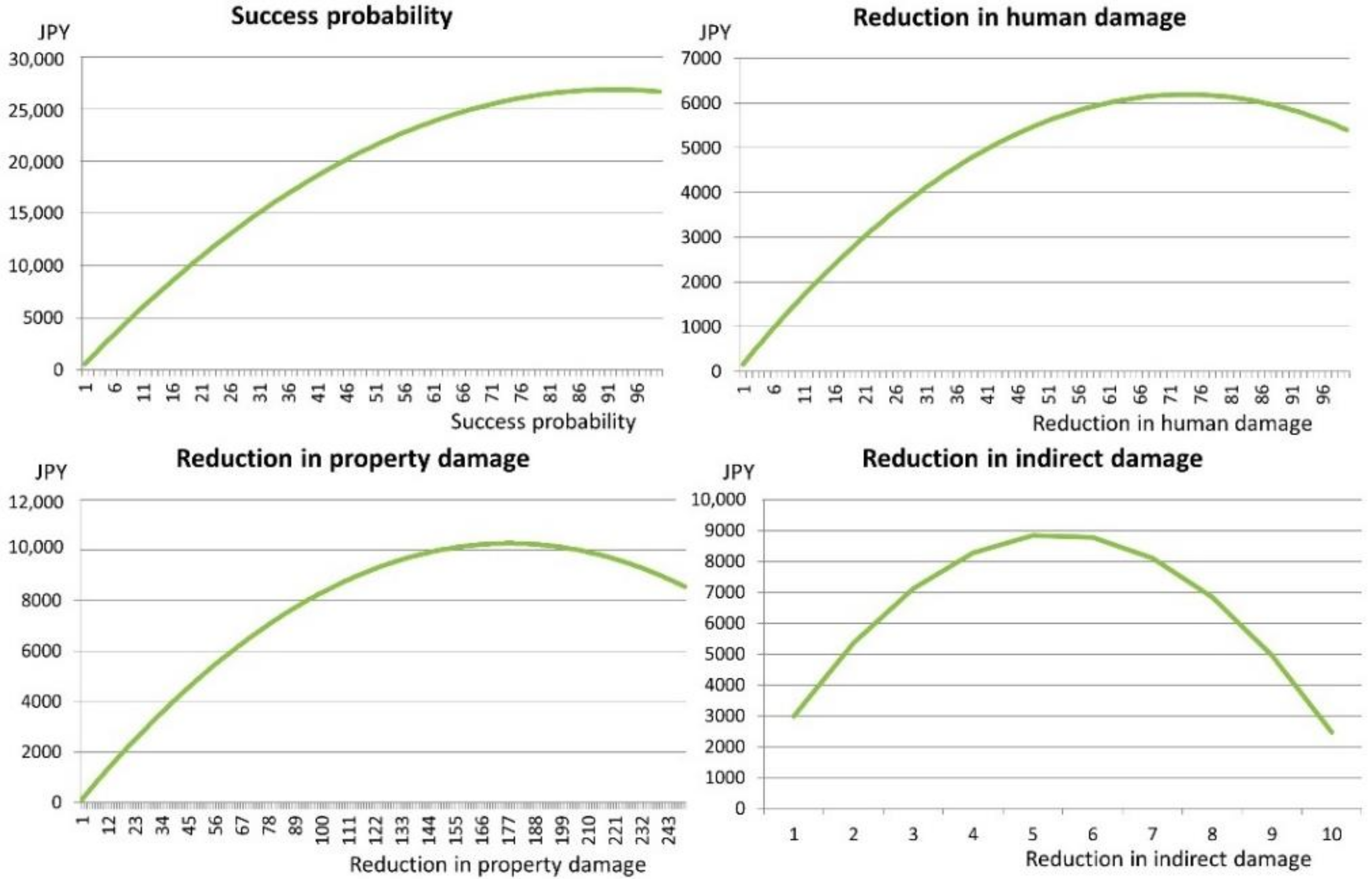
3.1. Estimation Using the CL and the RPL Models

For estimation, we used the CL and RPL models. In the RPL, variables other than the payment amount were assumed to be random parameters, and a normal distribution was assumed for the distribution of the random parameters. Additionally, six responses from one respondent were treated as panel data, and the estimation was performed using Halton draws with 100 iterations [47]. Nlogit6 (Econometric Software Inc, New York, U.S.) was used for the estimation.

Considering the possibility that the effects of success probability and each damage reduction on utility are nonlinear, we estimated a quadratic model that included the squared terms of success probability and each damage reduction, in addition to a linear model that assumed linearity in the deterministic term of the utility function.

The estimation results for RPL showed that the standard deviation (SD) parameters were statistically significant for most variables. In addition, McFadden’s pseudo-R-squared was larger for RPL than for CL in both linear and nonlinear models. Therefore, we discuss the results of the RPL.

The results for RPL showed that the coefficients of all squared terms were significant. Moreover, McFadden’s pseudo-R-squared value was larger in the quadratic model (0.2565) than in the linear model (0.2524). Therefore, we discuss the results of the quadratic model estimated using the RPL.

The estimation results for the quadratic model with CL and RPL models are shown in

Table 3. Estimation results of the quadratic model using the conditional logit (CL) and random parameter logit (RPL) models.

	CL	RPL
		Mean Parameter	SD Parameter	SD Parameter/Mean Parameter	MWTP (JPY)
Variables	Coefficient (Standard error)	Coefficient (Standard error)
ASC3	−0.12663 * (0.06679)	−1.20972 *** (0.11111)	4.03230 *** (0.09574)	−3.33	−24,041.5
Sports park	0.14690 *** (0.01266)	0.21166 *** (0.01672)	0.37644 *** (0.02802)	1.78	4206.4
Bird sanctuary	0.02201 * (0.01206)	0.02520 (0.01759)	0.50373 *** (0.02580)	-	500.8
Success probability	0.01632 *** (0.00164)	0.02941*** (0.00242)	0.00877 *** (0.00217)	0.30	584.5
Reduction in human damage	0.913 × 10−4 (0.00184)	0.00846 *** (0.00252)	0.01252 *** (0.00080)	1.48	168.1
Reduction in property damage	0.00363 *** (0.00065)	0.00582 *** (0.00085)	0.00218 *** (0.00073)	0.37	115.7
Reduction in indirect damage	0.09913 *** (0.01340)	0.16533 *** (0.01747)	0.02716 (0.01954)	-	3285.7
Success probability squared	−0.00010 *** (0.131 × 10−4)	−0.00016 *** (0.179 × 10−4)	0.829 × 10−4 *** (0.157 × 10−4)	−0.52	−3.2
Reduction in human damage squared	0.685 × 10−5 (0.152 × 10−4)	−0.574 × 10−4 *** (0.208 × 10−4)	0.561 × 10−5 (0.150 × 10−4)	-	−1.1
Reduction in property damage squared	−0.127 × 10−4 *** (0.218 × 10−5)	−0.164 × 10−4 *** (0.282 × 10−5)	0.498 × 10−5 ** (0.203 × 10−5)	−0.30	−0.3
Reduction in indirect damage squared	−0.00956 *** (0.00115)	−0.01529 *** (0.00153)	0.00324 ** (0.00129)	−0.21	−303.9
Amount of payment (one-time tax increase)	−0.394 × 10−4 *** (0.841 × 10−6)	−0.503 × 10−4 *** (0.112 × 10−5)	-
Number of individuals (Number of choice data)	5224 (31,344)	5224 (31,344)
Log-likelihood	−32,589.68	−25,601.252
McFadden’s pseudo-R-squared	0.0496	0.2565

Note 1: ***, **, and * indicate significance at the 1, 5, and 10% levels, respectively. Note 2: 1 JPY = 0.0087 USD (as of 30 January 2021).

. First, with respect to the mean parameters, ASC₃ is a constant term specific to alternative 3 (No project), which was found to be negative and significant. This indicates that the respondents favored implementing flood control projects regardless of the content.

The two other utilization possibilities of “use as a bird sanctuary” and “use as a sports park” were coded with effect codes, and “none” was excluded from the estimation [50]. Our findings show that the coefficient for “use as a sports park” was positive and significant, while the coefficient for “use as a bird sanctuary” was not significant. The coefficient of “none” was calculated as −0.21166−0.0252 = −0.23686 from the coefficients [50]. Therefore, the difference between the coefficients of “none” and “use as a sports park” was calculated to be 0.44852, and the difference between the coefficients of “none” and “use as a bird sanctuary” was calculated to be 0.26206.

The terms “success probability,” “reduction in human damage,” “reduction in property damage,” and “reduction in indirect damage” were all positive and significant, with their quadratic terms being negative and significant. This indicates that the marginal utility of these attributes is nonlinear and depends on the level of each attribute, that is, as each attribute is improved, the utility increases; however, the amount of increase in utility diminishes and eventually reaches a peak. The point at which utility peaks, that is, when the marginal utility reaches zero, is 91.9% for the “success probability,” 73.7 people for “reduction in human damage,” 177.5 houses for “reduction in property damage,” and 5.4 days for “reduction in indirect damage.” The peak of the “success probability” is approximately 92%, which is close to 100%; the higher the success probability, the more desirable it is.

As expected, the “amount of payment” was negative and significant. This means that an increase in payments leads to a decrease in utility. The absolute value of this estimate represents the marginal utility of income. Using this estimate, we calculated the MWTP for each variable.

Next, we consider the SD parameters. The significance of the SD parameters indicates that the preferences for the variable are heterogeneous among respondents. In our study, except for the “reduction in indirect damage” and the quadratic term for “reduction in human damage,” the SD parameters were significant. Therefore, we can conclude that preferences are heterogeneous for most variables.

To understand the magnitude of the heterogeneity in preferences, the ratios of the SD parameters to the mean parameters were calculated for variables where both the mean and SD parameters were significant. ASC₃ had a relatively high ratio, indicating the heterogeneous preferences among respondents for not implementing any project. Further, of the three types of damage reduction, “reduction in human damage” had a relatively large heterogeneity in preferences. The ratio for “bird sanctuary” was not calculated as the mean parameter was not significant; however, since the coefficient of the SD parameter was a large value while the mean parameter was not significant, we can assume that the preference for “bird sanctuary” is very heterogeneous.

The MWTPs calculated based on the estimates of the mean parameters are shown in the rightmost column of Table 3. MWTPs for “use as a sports park” and “use as a bird sanctuary” were JPY 4206.45 and JPY 500.81, respectively. Since the coefficient of “none” was calculated to be −0.23686, as explained earlier, MWTP for “none” was JPY −4707.3. Therefore, the difference in WTP between “use as a sports park” and “none” was calculated to be JPY 8913.7, and the difference in WTP between “use as a bird sanctuary” and “none” was calculated to be JPY 5208.1.

Since the preferences for “success probability” and each damage reduction are quadratic, the MWTP depends on the value of each variable. This means that there are benefits from improvements in these variables; however, benefits from additional improvements are diminishing. Since it is easier to understand the MWTP for these improvements if we access them visually, the WTPs for success probability and each damage reduction are illustrated in Figure 2.

Using these MWTPs, we could estimate the benefits of various flood control projects. As an example, let us estimate the benefits of “Project 2” (benefit from the change from “No project” to “Project 2”) in Figure 1. Using the MWTP estimates in Table 3, the benefit of changing from “none” to “use as a sports park” is calculated to be JPY 8913.7, the benefit of changing the probability from 100% to 80% is JPY −242.46, the benefit of 20 fewer people suffering damage is JPY 2906.2, the benefit of 200 fewer houses suffering property damage is JPY 10,097.4, and the benefit of reducing indirect damage by 7 days is JPY 8110.4. Therefore, the benefit of “Project 2” is JPY 29,785 per household.

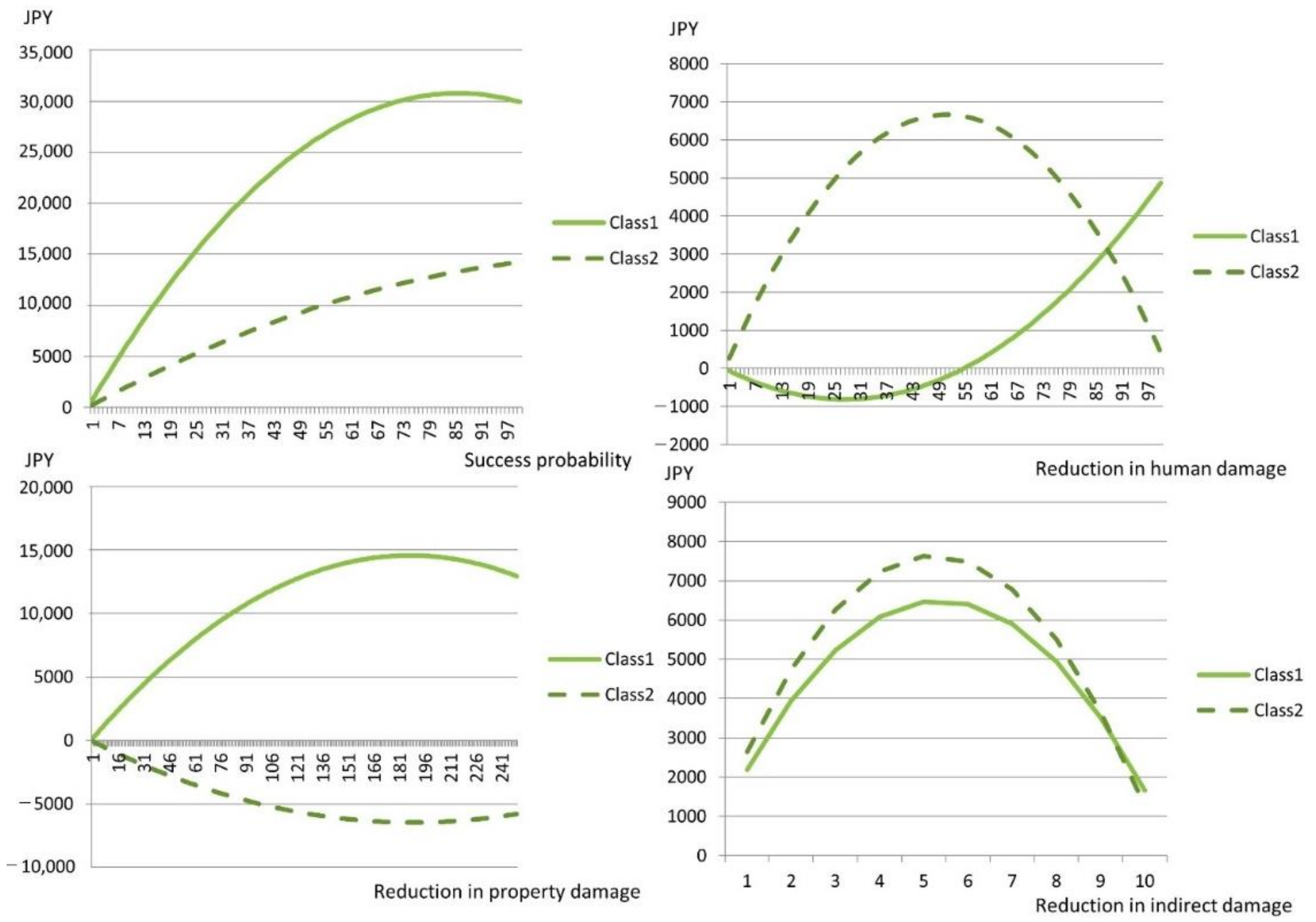
3.2. Estimation Using the LCM

The estimation result of the RPL verified the existence of heterogeneity in the preferences for most attributes. To deepen our understanding of heterogeneity in preferences, we performed an estimation using an LCM. The membership function estimated in the LCM can reveal factors related to heterogeneity in preferences. Stata16 (StataCorp LLC, Texas, U.S.) and lclogit2, a Stata command for fitting LCM via the expectation-maximization algorithm [51] was used for the estimation.

The variables used in the membership function included a male dummy (male), indicating that the respondent is male, a continuous variable representing the respondents’ age (age), and a direct damage dummy (direct) that takes a value of 1, when the respondent lives in an area that may be directly affected by the flood.

The number of classes in an LCM should be determined based on an overall assessment, considering the ease of interpretation and information criteria, such as Bayesian information criterion (BIC) [52,53]. In this study, models with two to five classes were estimated.

As the number of classes increases, the information criteria (BIC, Akaike information criterion (AIC), and corrected AIC (cAIC)) become smaller; however, the classes become more fragmented and harder to interpret. Therefore, we focused on the ease of interpretation and adopted the results of the 2-class model.

Table 4. Estimation results of the quadratic model using the LCM.

	Class 1		Class 2
Variables	Coefficient (Standard Error)	MWTP (JPY)	Coefficient (Standard Error)	MWTP (JPY)
Utility function
ASC3	−1.71160 *** (0.07995)	−42261.8	1.74039 *** (0.24276)	14,625.2
Sports park	0.20235 *** (0.01430)	4996.4	−0.06055 (0.05731)	−508.9
Bird sanctuary	0.02270 * (0.01358)	560.4	0.08847 * (0.05319)	743.5
Success probability	0.02912 *** (0.00213)	718.9	0.02808 *** (0.00729)	236.0
Reduction in human damage	−0.00239 (0.00223)	-59.0	0.03151 *** (0.00721)	264.7
Reduction in property damage	0.00630 *** (0.00077)	155.6	−0.00821 *** (0.00267)	−69.0
Reduction in indirect damage	0.09802 *** (0.01594)	2420.3	0.35126 *** (0.05490)	2951.7
Success probability squared	−0.00017 *** (0.155 × 10−4)	-4.3	−0.00011 ** (0.572 × 10−4)	−1.0
Reduction in human damage squared	0.436 × 10−4 ** (0.183 × 10−4)	1.1	−0.00031 *** (0.605 × 10−4)	−2.6
Reduction in property damage squared	−0.168 × 10−4 *** (0.251 × 10−5)	-0.4	0.217 × 10−4 ** (0.940 × 10−5)	0.2
Reduction in indirect damage squared	−0.00913 *** (0.00138)	-225.5	−0.03359 *** (0.00479)	−282.2
Amount of payment (one-time tax increase)	−0.00004 *** (0.911 × 10−6)		−0.00012 *** (0.976 × 10−5)
Membership function
Constant	0.51631 *** (0.12035)		0 -
Male	−0.12161 * (0.06491)		0 -
Age	0.01049 *** (0.00236)		0 -
Live in a place that may be directly affected by floods	0.33041 *** (0.08837)		0 -
Class probabilities	0.73		0.27
Number of individuals (Number of choice data)	5224 (31,344)
Log-likelihood	−26,183.152
McFadden’s pseudo-R-squared	0.2396

Note 1: ***, **, and * indicate significance at the 1, 5, and 10% levels, respectively. Note 2: 1 JPY = 0.0087 USD (as of 30 January 2021).

presents the estimation results and the MWTPs calculated based on the parameter estimates.

First, we consider the estimation result of the membership function. The coefficients of class 1 are estimated as the relative coefficients when the coefficients of each variable in the membership function of class 2 are set to 0.

In Class 1, the constant, age, and direct damage dummy were positive and significant at the 1% level. In addition, the male dummy was negative and significant at the 10% level. These results indicate that females, older people, and people living in areas that may be directly affected by floods, have a relatively higher probability of belonging to Class 1.

Next, we examine the estimation results for the deterministic term of the utility function. For utilization purposes other than DRR, in Class 1, both the sports park and bird sanctuary were positive and significant at the 1% and 10% levels, respectively. The coefficient was larger for the sports park, indicating that it is more preferred. In contrast, in Class 2, the sports park was not significant, while the bird sanctuary was positive and significant at the 10% level, indicating that the bird sanctuary is more preferred. These variables were coded with effect codes and “none” was excluded from the estimation; therefore, the difference in WTP between “use as a sports park” and “none” and the difference in WTP between “use as a bird sanctuary” and “none” were calculated in the same way, as in the case of RPL.

The quadratic terms for “success probability” and each damage reduction were significant. WTPs depends on the value of each variable and are illustrated in Figure 3. Note that we used the coefficient for “reduction in human damage” in Class 1, which is not significant in this calculation.

From the figure, we can see that there are significant differences in preferences among classes. Class 1, in which people who live in an area that may be directly affected by floods, tends to have a higher MWTP for the “success probability” than Class 2.

As for the “reduction in human damage,” Class 2 has a relatively high MWTP for small improvements, peaking at approximately 50 people, whereas Class 1 has a negative MWTP for small improvements, a positive MWTP after 50 people, and an accelerating magnitude as improvements are made. Class 1, which is likely to include people living in areas that may be directly affected by floods, is expected to highly appreciate improvement above a certain level.

As for the “reduction in property damage,” the MWTP is larger for Class 1 than for Class 2. In contrast, for “reduction in indirect damage,” the MWTP is greater for Class 2 than for Class 1. This may be because people who live in areas that are not directly affected by floods still suffer indirect damage.

These results indicate that people in Class 1 highly value the “success probability” and reduction in direct damage (human and property damage), whereas people in Class 2 have a higher preference for “reduction in indirect damage.” This difference in preference may reflect the differences in damage that people in each class are likely to suffer.

At the 1% level, ASC₃ was negative and significant for Class 1, whereas it was positive and significant for Class 2. This indicates that people in Class 1 prefer to implement a project regardless of the content, whereas people in Class 2 prefer not to implement any project regardless of the content. This can be attributed to the fact that Class 1, which is more likely to suffer direct damage, is proactive in implementing flood control projects, whereas Class 2, which is less likely to suffer direct damage, is reluctant to implement flood control projects that would incur a financial burden.

4. Conclusions

In this study, we conducted a questionnaire survey to investigate public preferences with respect to DRR and its uncertainty. Using the CE, we obtained the following results: (1) when there are no floods, the use of the area of the flood control project as a sports park was highly evaluated; (2) benefits were obtained from the increase in “success probability,” and the reduction in “human damage,” “property damage,” and “indirect damage;” however, benefits obtained from additional improvements diminished; (3) preferences for DRR and its uncertainty were heterogeneous among respondents; (4) the segment that includes more women, older people, and more people who live in the areas that may be directly affected by floods had higher ratings for “success probability” and relatively slightly lower ratings for “reduction in indirect damage.”

Using our results, we were able to explain the public preferences for DRR and its uncertainty and assess the benefits of various DRR measures with uncertainty.

Our results have several important implications for policymakers. First, this study revealed that flood control, including Eco-DRR, provides significant benefits to citizens. The cost-effectiveness of such flood control may be sufficiently high to ensure that its implementation deserves consideration.

Second, the results indicate that the use of the area as a sports park or bird sanctuary provides significant benefits compared to when the area is just used for flood control. Therefore, it is suggested that when planning flood control measures, the area is utilized for purposes other than flood control. It is important to maximize the benefits derived from flood control facilities during normal times to maximize the net benefits derived from flood control projects.

This is also important in terms of the acceptability of the project and consensus building in the community. The project will be more acceptable to local residents if it is implemented the way they desire because it will increase the benefits they derive from it. This may be especially important in green infrastructures that are characterized by multifunctionality.

Third, while it was expectedly found that uncertainty in DRR was negatively evaluated, it was also found that uncertainty in the effects does not mean that such projects will never be accepted. Our analysis shows that even projects with uncertain effects are acceptable to individuals if the effects of flood control measures are sufficiently large, or if their use for non-disaster prevention purposes is sufficiently attractive. This suggests that when considering the implementation of DRR measures with uncertain effects, it is important not to give up implementation because of the element of uncertainty, but to increase the effectiveness of disaster prevention or make other uses more attractive. This indicates that green infrastructures, which are characterized by the presence of uncertainty in DRR, have the potential to become widespread.

Fourth, the LCM results revealed that people had different preferences for flood control. This result suggests that sufficient discussion is required to reach a consensus. Even if cost-benefit analysis shows that the project is efficient, consensus building in the community is necessary for its actual implementation. Our results demonstrated the importance of this process.

Additionally, this study adds valuable contributions to the scarce research on economic valuation of DRR with green infrastructures, demonstrating the usefulness of CE as an analytical method. Thus, our research not only provides implications for policymakers but also contributes to the development of academic research on green infrastructures.

Nevertheless, this study has some limitations that need to be addressed. First, in this research, human damage is defined as the total number of dead, missing, or injured people; property damage is defined as the total number of houses that are totally destroyed, partially destroyed, partially damaged, or flooded above or below floor level; and indirect damage is defined as damage that occurs in a wide range of areas due to power and water outages, sewage treatment facility shutdowns, and disruptions of bridges and roads. However, it is highly likely that people evaluate the reduction in the number of deaths differently from the reduction in the number of injuries. Thus, future research should conduct surveys that categorize human, property, and indirect damage in greater detail.

Second, we focus on flood control, and its results may not be generalizable to green infrastructures against other disasters. For example, a rise in sea level due to climate change may increase the damage caused by tsunamis and storm surges. Therefore, the use of green infrastructure in coastal areas, including coastal forests, is an important issue to be addressed in the future. In addition to disasters, urban greening is becoming increasingly important as a countermeasure to rising temperatures in urban areas. Therefore, future research on green infrastructure in fields other than flood control is required.

Third, this study used an LCM to show that people who live in areas that may be directly affected by floods and those who do not live in such area have different preferences, but a more detailed analysis is needed on this point. An analysis of how preferences change as one moves away from the center of damage, that is, an analysis of the distance decay of the MWTP for each attribute, would be useful to improve the accuracy of the assessment of the benefits of flood control projects.

References

1. Mercer, J. Disaster risk reduction or climate change adaptation: Are we reinventing the wheel? J. Int. Dev. 2010, 22, 247–264. [Google Scholar] [CrossRef]
2. Kelman, I. Climate change and the Sendai framework for disaster risk reduction. Int. J. Disast. Risk Sc. 2015, 6, 117–127. [Google Scholar] [CrossRef] [Green Version]
3. IUCN. Global Standard for Nature-based Solutions. In A User-Friendly Framework for the Verification, Design and Scaling Up of NbS, 1st ed.; IUCN: Gland, Switzerland, 2020. [Google Scholar]
4. Anderson, C.C.; Renaud, F.G. A review of public acceptance of nature-based solutions: The ‘why’, ‘when’ and ‘how’ of success for disaster risk reduction measures. Ambio 2021, 50, 1552–1573. [Google Scholar] [CrossRef] [PubMed]
5. Temmerman, S.; Meire, P.; Bouma, T.J.; Herman, P.M.; Ysebaert, T.; De Vriend, H.J. Ecosystem-based coastal defence in the face of global change. Nature 2013, 504, 79–83. [Google Scholar] [CrossRef] [PubMed]
6. Barbier, E.B. Valuing the storm protection service of estuarine and coastal ecosystems. Ecosyst. Serv. 2015, 11, 32–38. [Google Scholar] [CrossRef]
7. Reguero, B.G.; Beck, M.W.; Bresch, D.N.; Calil, J.; Meliane, I. Comparing the cost effectiveness of nature-based and coastal adaptation: A case study from the Gulf Coast of the United States. PLoS ONE 2018, 13, e0192132. [Google Scholar] [CrossRef] [Green Version]
8. Ministry of the Environment, Government of Japan. Ecosystem-based Disaster Risk Reduction in Japan: A Handbook for Practitioners; Ministry of the Environment, Government of Japan: Tokyo, Japan, 2016.
9. Cohen, J.P.; Field, R.; Tafuri, A.N.; Ports, M.A. Cost comparison of conventional gray combined sewer overflow control infrastructure versus a green/gray combination. J. Irrig. Drain Eng. 2012, 138, 534–540. [Google Scholar] [CrossRef]
10. United States Environmental Protection Agency. Case Studies Analyzing the Economic Benefits of Low Impact Development and Green Infrastructure Programs; United States Environmental Protection Agency: Washington, DC, USA, 2013.
11. Jayasooriya, V.M.; Ng, A.W. Tools for modeling of stormwater management and economics of green infrastructure practices: A review. Water Air Soil Pollut. 2014, 225, 1–20. [Google Scholar] [CrossRef] [Green Version]
12. Nordman, E.E.; Isley, E.; Isley, P.; Denning, R. Benefit-cost analysis of stormwater green infrastructure practices for grand rapids, Michigan, USA. J. Clean Prod. 2018, 200, 501–510. [Google Scholar] [CrossRef]
13. Li, C.; Peng, C.; Chiang, P.C.; Cai, Y.; Wang, X.; Yang, Z. Mech. and applications of green infrastructure practices for stormwater control: A review. J. Hydrol. 2019, 568, 626–637. [Google Scholar] [CrossRef]
14. Onuma, A.; Tsuge, T. Comparing green infrastructure as ecosystem-based disaster risk reduction with gray infrastructure in terms of costs and benefits under uncertainty: A theoretical approach. Int. J. Disast. Risk Reduct. 2018, 32, 22–28. [Google Scholar] [CrossRef]
15. Dhakal, K.P.; Chevalier, L.R. Managing urban stormwater for urban sustainability: Barriers and policy solutions for green infrastructure application. J. Environ. Manag. 2017, 203, 171–181. [Google Scholar] [CrossRef] [PubMed]
16. da Silva, J.M.C.; Wheeler, E. Ecosystems as infrastructure. Perspect Ecol. Conserv. 2017, 15, 32–35. [Google Scholar] [CrossRef]
17. United States Environmental Protection Agency. Managing Wet Weather with Green Infrastructure: Action Strategy; United States Environmental Protection Agency: Washington, DC, USA, 2008.
18. City of Portland Bureau of Environmental Services. Portland’s Green Infrastructure: Quantifying the Health, Energy, and Community Livability Benefits; City of Portland Bureau of Environmental Services: Oregon, Portland, 2010.
19. European Commission. Communication from the Commission to the European Parliament, the Council, the European Economic and Social Committee and the Committee of the Regions, Green Infrastructure (GI)—Enhancing Europe’s Natural Capital; European Commission: Brussels, Belgium, 2013. [Google Scholar]
20. Ministry of Land, Infrastructure, Transport and Tourism, Government of Japan. National Spatial Strategy (National Plan); Ministry of Land, Infrastructure, Transport and Tourism, Government of Japan: Tokyo, Japan, 2015.
21. Setagaya City. Setagaya City Countermeasures of Torrential Rainfall Action Plan (FY 2018–2021); Setagaya City: Tokyo, Japan, 2018. [Google Scholar]
22. Ying, J.; Zhang, X.; Zhang, Y.; Bilan, S. Green infrastructure: Systematic literature review. Econ. Res.-Ekon. Istraz. 2021, 1–22. [Google Scholar] [CrossRef]
23. Veronesi, M.; Chawla, F.; Maurer, M.; Lienert, J. Climate change and the willingness to pay to reduce ecological and health risks from wastewater flooding in urban centers and the environment. Ecol. Econ. 2014, 98, 1–10. [Google Scholar] [CrossRef] [Green Version]
24. Brouwer, R.; Bliem, M.; Getzner, M.; Kerekes, S.; Milton, S.; Palarie, T.; Palariee, T.; Szerényid, Z.; Vadineanue, A.; Wagtendonk, A. Valuation and transferability of the non-market benefits of river restoration in the Danube river basin using a choice experiment. Ecol. Eng. 2016, 87, 20–29. [Google Scholar] [CrossRef]
25. Brent, D.A.; Gangadharan, L.; Lassiter, A.; Leroux, A.; Raschky, P.A. Valuing environmental services provided by local stormwater management. Water Resour. Res. 2017, 53, 4907–4921. [Google Scholar] [CrossRef]
26. Valasiuk, S.; Czajkowski, M.; Giergiczny, M.; Żylicz, T.; Veisten, K.; Landa Mata, I.; Halse, A.H.; Elbakidze, M.; Angelstam, P.; Angelstam, P. Is forest landscape restoration socially desirable? A discrete choice experiment applied to the Scandinavian transboundary Fulufjället National Park Area. Restor Ecol. 2018, 26, 370–380. [Google Scholar] [CrossRef] [Green Version]
27. Meng, T.; Hsu, D. Stated preferences for smart green infrastructure in stormwater management. Landsc. Urban Plan 2019, 187, 1–10. [Google Scholar] [CrossRef]
28. Shr, Y.H.; Ready, R.J.; Orland, B.; Echols, S. How do visual representations influence survey responses? evidence from a choice experiment on landscape attributes of green infrastructure. Ecol. Econ. 2019, 156, 375–386. [Google Scholar] [CrossRef]
29. Pienaar, E.F.; Soto, J.R.; Lai, J.H.; Adams, D.C. Would county residents vote for an increase in their taxes to conserve native habitat and ecosystem services? Funding conservation in palm beach county, Florida. Ecol. Econ. 2019, 159, 24–34. [Google Scholar] [CrossRef]
30. Ando, A.W.; Cadavid, C.L.; Netusil, N.R.; Parthum, B. Willingness-to-volunteer and stability of preferences between cities: Estimating the benefits of stormwater management. J. Environ. Econ. Manag. 2020, 99, 102274. [Google Scholar] [CrossRef]
31. Deely, J.; Hynes, S. Blue-green or grey, how much is the public willing to pay? Landsc. Urban Plan. 2020, 203, 103909. [Google Scholar] [CrossRef]
32. Wieczerak, T.; Lal, P.; Witherell, B.; Oluoch, S. Public preferences for green infrastructure improvements in Northern New Jersey: A discrete choice experiment approach. SN Soc. Sci. 2022, 2, 1–20. [Google Scholar] [CrossRef]
33. Holmes, T.P.; Adamowicz, W.L.; Carlsson, F. Choice experiments. In A Primer on Nonmarket Valuation, 2nd ed.; Champ, P.A., Boyle, K.J., Brown, T.C., Eds.; Springer: Dordrecht, The Netherlands, 2017; pp. 133–186. [Google Scholar]
34. Ganderton, P.T. ‘Benefit–cost analysis’ of disaster mitigation: Application as a policy and decision-making tool. Mitig. Adapt. Strateg. Glob. Chang. 2005, 10, 445–465. [Google Scholar] [CrossRef]
35. Mechler, R. Cost-Benefit Analysis of Natural Disaster Risk Management in Developing Countries; Deutsche Gesellschaft für Technische Zusammenarbeit (GTZ): Eschborn, Germany, 2005. [Google Scholar]
36. Benson, C.; Twigg, J. Tools for Mainstreaming Disaster Risk Reduction: Guidance NOTES for development Organisations; ProVention Consortium: Geneva, Switzerland, 2007. [Google Scholar]
37. Moench, M.; Mechler, R.; Stapelton, S. Costs and benefits of disaster risk reduction. In UN/ISDR Information Note to the Global Platform for Disaster Risk Reduction, No. 3; United Nations Office for Disaster Risk Reduction (UNISDR): Geneva, Switzerland, 2007. [Google Scholar]
38. Rose, A.; Porter, K.; Dash, N.; Bouabid, J.; Huyck, C.; Whitehead, J.; Shaw, D.; Eguchi, R.; Taylor, C.; McLane, T.; et al. Benefit-cost analysis of FEMA hazard mitigation grants. Nat. Hazards Rev. 2007, 8, 97–111. [Google Scholar] [CrossRef] [Green Version]
39. Shreve, C.M.; Kelman, I. Does mitigation save? Reviewing cost-benefit analyses of disaster risk reduction. Int. J. Disast. Risk Re 2014, 10, 213–235. [Google Scholar] [CrossRef] [Green Version]
40. Wethli, K. Benefit-Cost Analysis for Risk Management: Summary of Selected Examples; Background paper for the World Development Report 2014; World Bank: Washington, DC, USA, 2014. [Google Scholar]
41. Hugenbusch, D.; Neumann, T. Cost-Benefit Analysis of Disaster Risk Reduction: A Synthesis for Informed Decision Making; Aktion Deutschland Hilft: Bon, Germany, 2016. [Google Scholar]
42. Mechler, R. Reviewing estimates of the economic efficiency of disaster risk management: Opportunities and limitations of using risk-based cost–benefit analysis. Nat. Hazards 2016, 81, 2121–2147. [Google Scholar] [CrossRef] [Green Version]
43. Kim, H.; Shoji, Y.; Tsuge, T.; Kubo, T.; Nakamura, F. Relational values help explain green infrastructure preferences: The case of managing crane habitat in Hokkaido, Japan. People Nat. 2021, 3, 861–871. [Google Scholar] [CrossRef]
44. Hensher, D.A.; Rose, J.M.; Greene, W.H. Applied Choice Analysis: A Primer; Cambridge University Press: Cambridge, UK, 2005. [Google Scholar]
45. McFadden, D. Conditional logit analysis of qualitative choice behavior. In Frontiers in Econometrics; Zarembka, P., Ed.; Academic Press: New York, NY, USA, 1973; pp. 105–142. [Google Scholar]
46. Revelt, D.; Train, K. Mixed logit with repeated choices: Households’ choices of appliance efficiency level. Rev. Econ. Stat. 1998, 80, 647–657. [Google Scholar] [CrossRef]
47. Train, K.E. Discrete Choice Methods with Simulation, 2nd ed.; Cambridge University Press: Cambridge, UK, 2009. [Google Scholar]
48. Swait, J. A structural equation model of latent segmentation and product choice for cross-sectional revealed preference choice data. J. Retail. Consum. Serv. 1994, 1, 77–89. [Google Scholar] [CrossRef]
49. Boxall, P.C.; Adamowicz, W.L. Understanding heterogeneous preferences in random utility models: A latent class approach. Environ. Resour. Econ. 2002, 23, 421–446. [Google Scholar] [CrossRef]
50. Beck, M.; Gyrd-Hanse, D. Effects coding in discrete choice experiments. Health Econ. 2005, 14, 1079–1083. [Google Scholar] [CrossRef]
51. Yoo, H.I. lclogit2: An enhanced command to fit latent class conditional logit models. Stata J. 2020, 20, 405–425. [Google Scholar] [CrossRef]
52. Scarpa, R.; Thiene, M. Destination choice models for rock climbing in the northeastern alps: A latent-class approach based on intensity of preferences. Land Econ. 2005, 81, 426–444. [Google Scholar] [CrossRef]
53. Hynes, S.; Hanley, N.; Scarpa, R. Effects on welfare measures of alternative means of accounting for preference heterogeneity in recreational demand models. Am. J. Agr. Econ. 2008, 90, 1011–1027. [Google Scholar] [CrossRef]
Figure 1. An example of a CE question.
Sustainability 14 04753 g001
Figure 2. WTPs calculated based on RPL estimation results. Note: 1 JPY = 0.0087 USD (as of 30 January 2021).
Sustainability 14 04753 g002
Figure 3. WTPs for success probability and each damage reduction by class. Note: 1 JPY = 0.0087 USD (as of 30 January 2021).
Sustainability 14 04753 g003