
Assessment of Climate Change Impact on the Annual Maximum Flood in an Urban River in Dublin, Ireland


Abstract
:1. Introduction
2. Materials and Methods
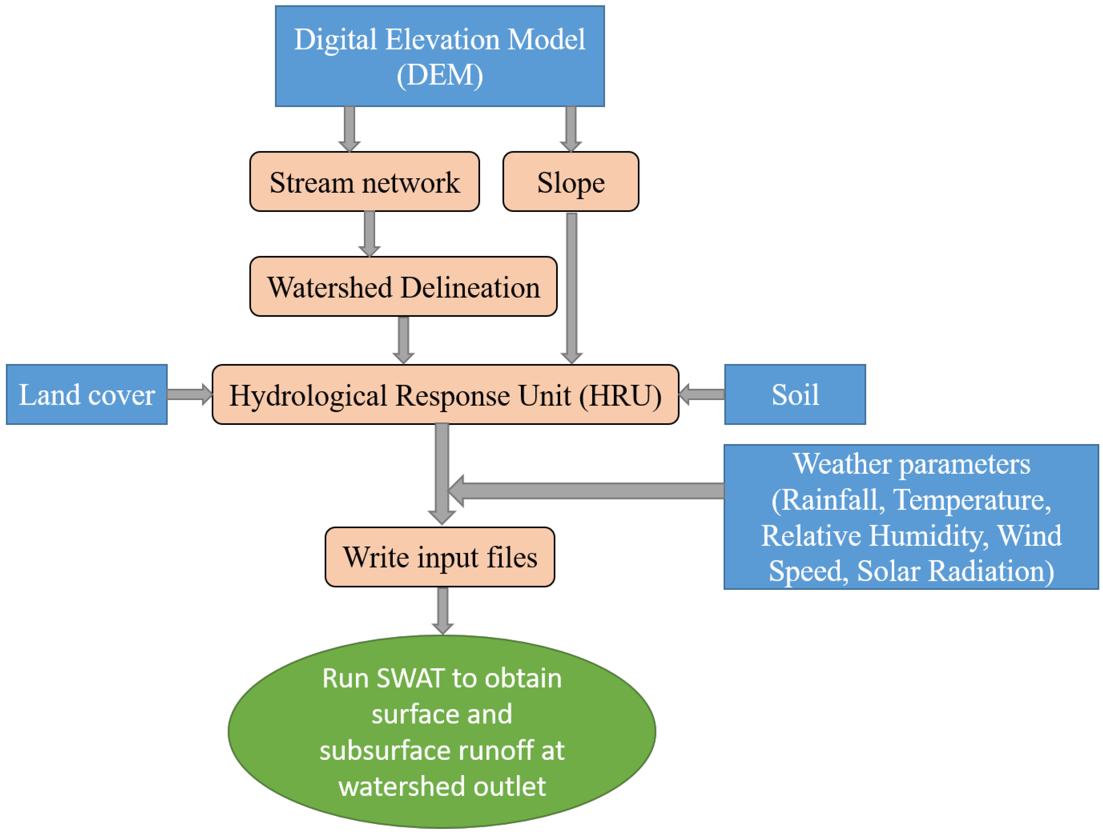
2.1. Soil Water Assessment Tool (SWAT) Model
- (a)
- Pearson correlation coefficient ():where is the observed runoff/streamflow at time , is the SWAT model predicted runoff at time , is the number of data points (daily/annual maximum), and is the mean observed flow.
- (b)
- Nash–Sutcliffe Efficiency ():
- (c)
- Kling–Gupta Efficiency ():where is the Pearson correlation coefficient, , and .
2.2. Quantile-Based Bias Correction
2.3. Generalised Extreme Value Distribution
2.4. Hydrological Engineering Centre—River Analysis System (HEC-RAS) Model
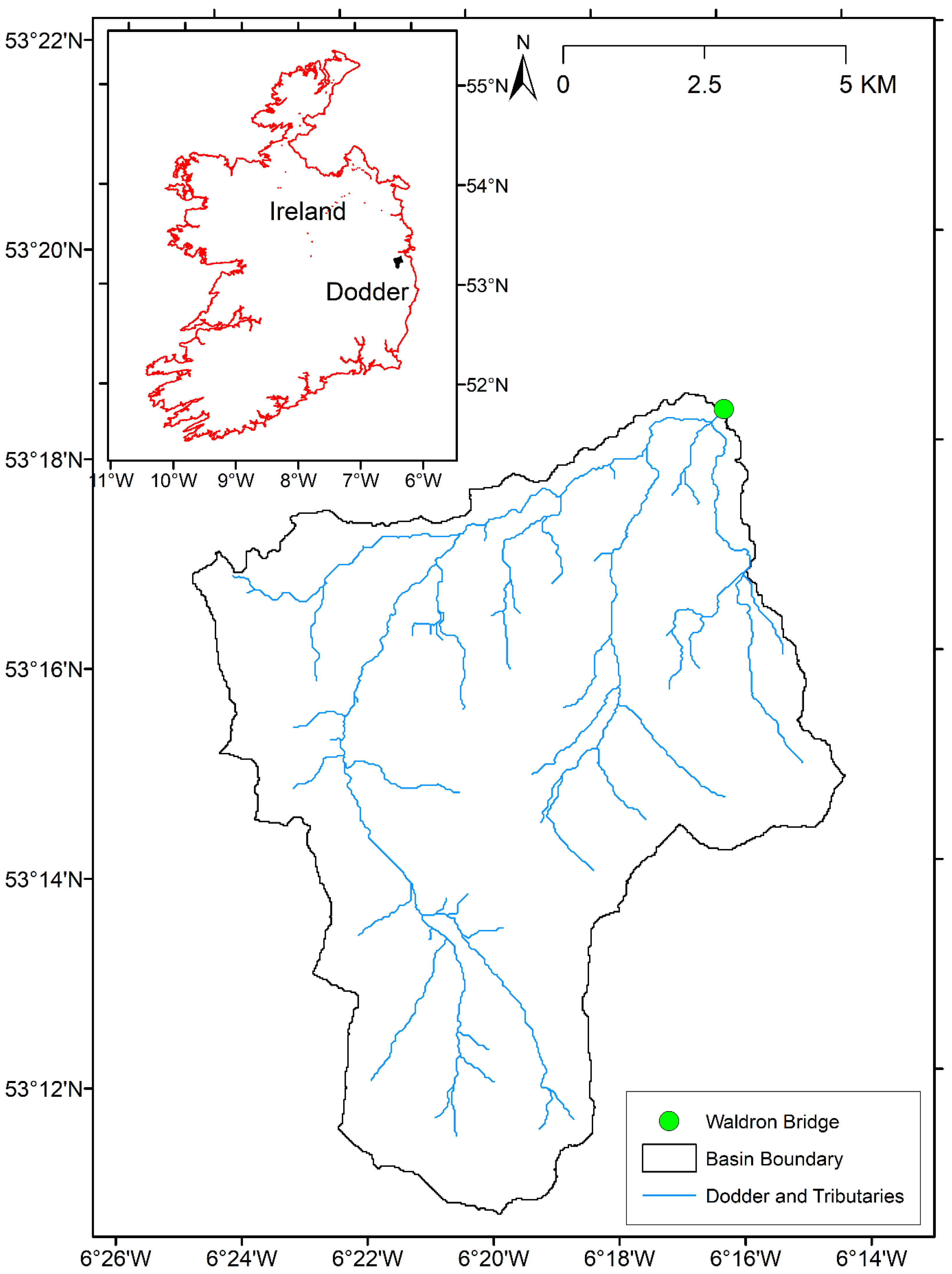
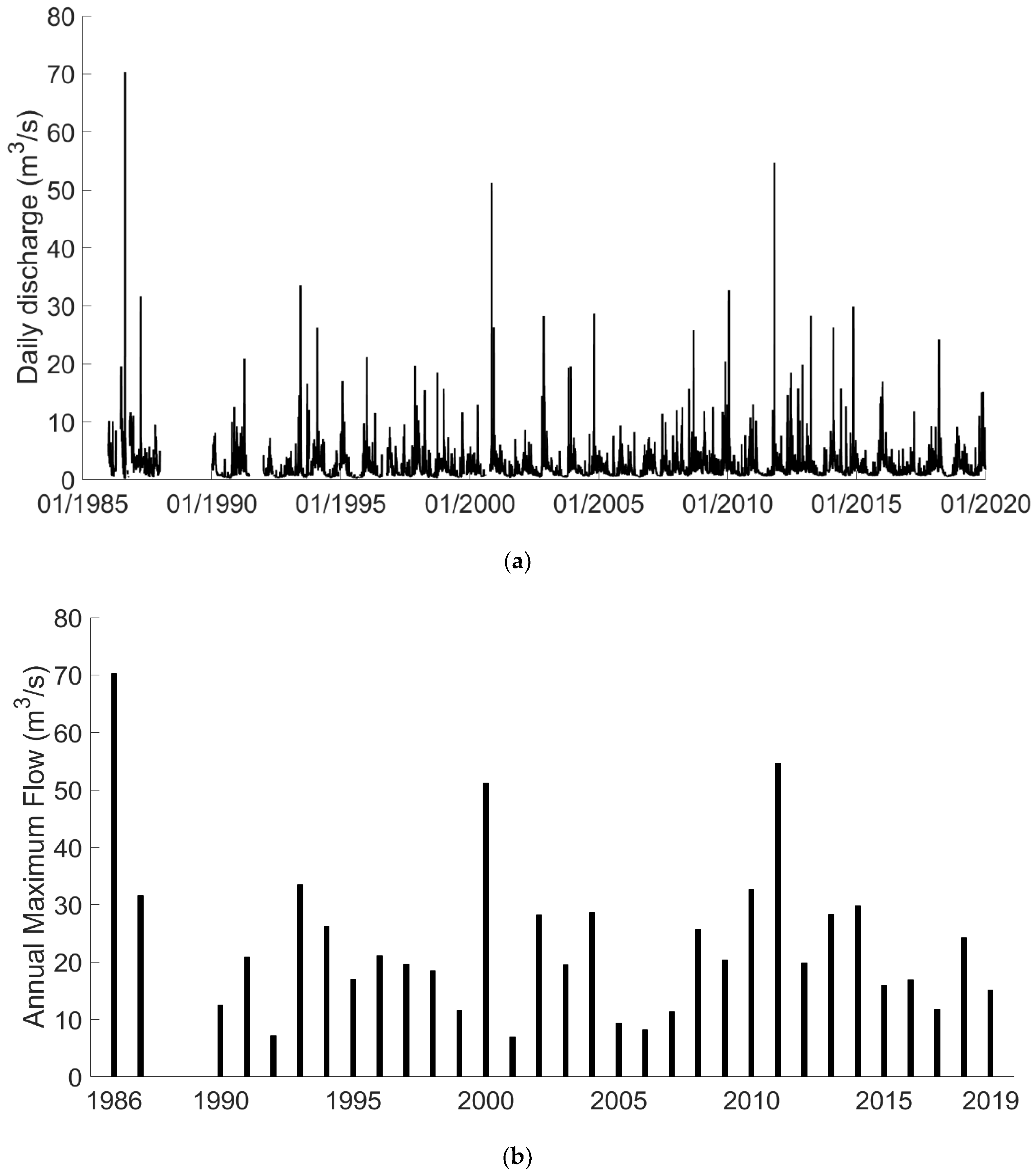
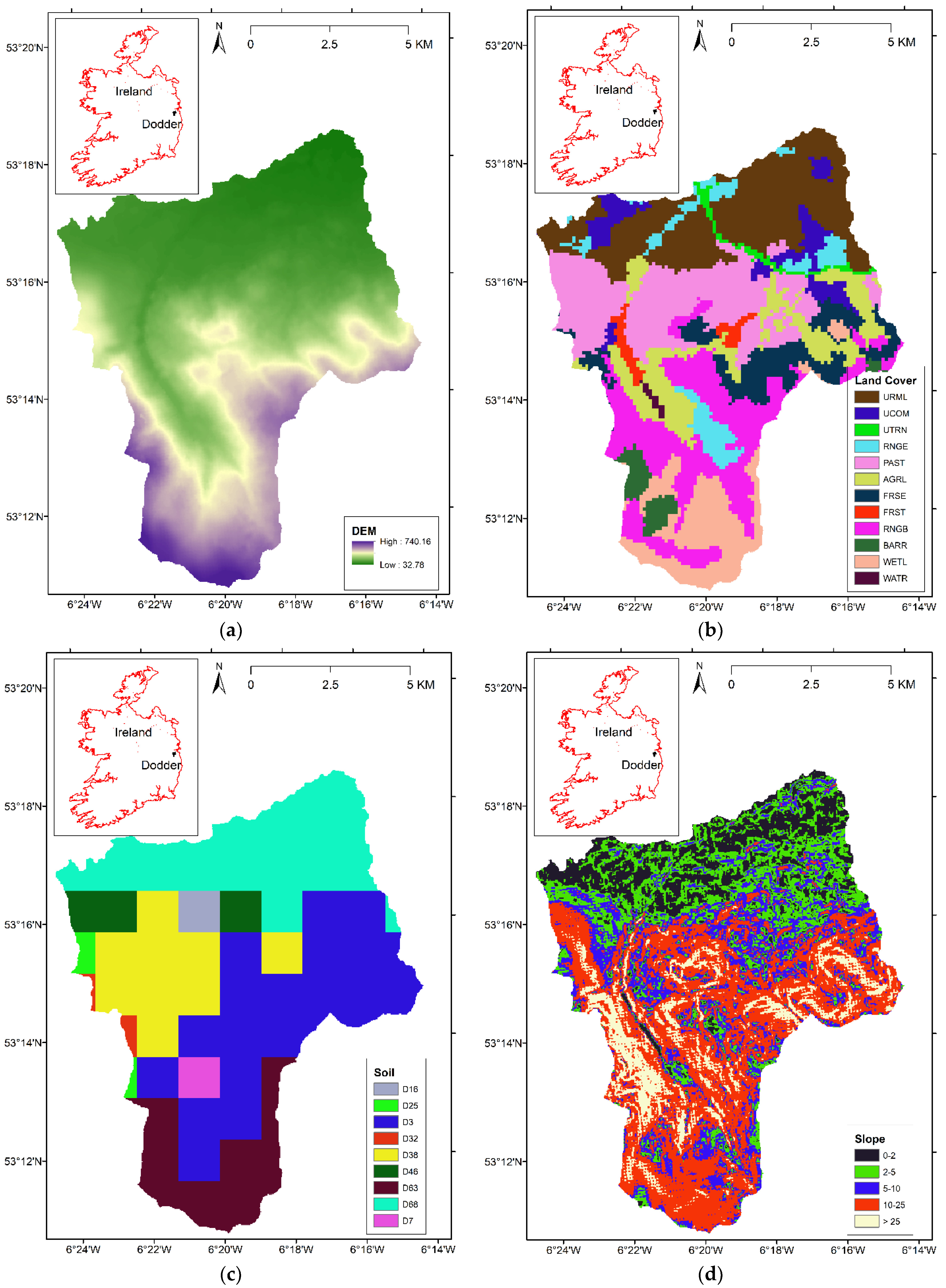
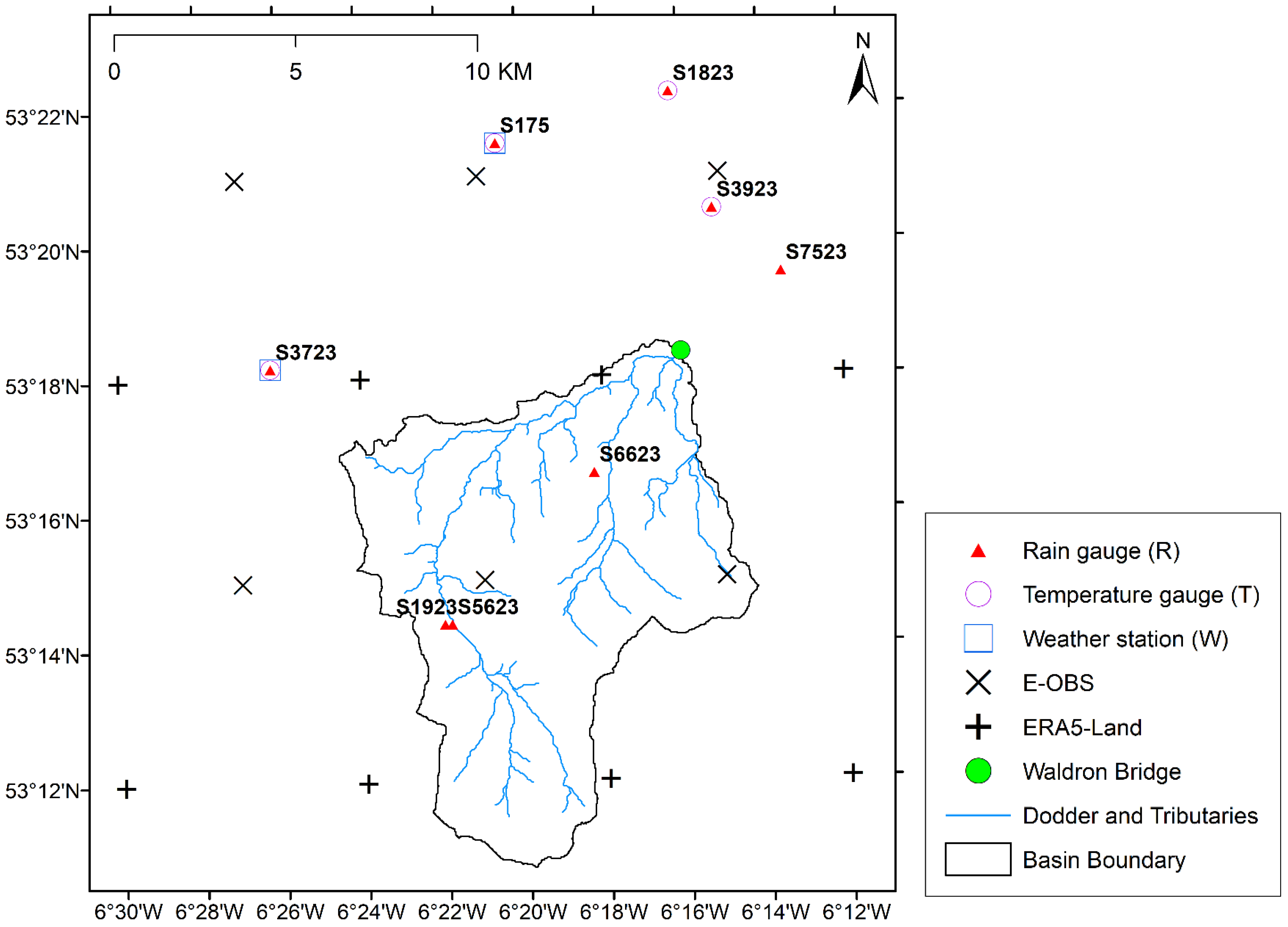
3. Catchment Description and Input Data
4. Results and Discussion
5. Conclusions
Supplementary Materials
Author Contributions
Funding
Data Availability Statement
Acknowledgments
Conflicts of Interest
References
- Hamlet, A.F.; Lettenmaier, D.P. Effects of climate change on hydrology and water resources in the Columbia river basin. JAWRA J. Am. Water Resour. Assoc. 1999, 35, 1597–1623. [Google Scholar] [CrossRef]
- Basu, B.; Nogal, M.; O’Connor, A. New approach to multisite downscaling of precipitation by identifying different set of atmospheric predictor variables. J. Hydrol. Eng. 2020, 25, 4020013. [Google Scholar] [CrossRef]
- Jahangir, M.H.; Reineh, S.M.M.; Abolghasemi, M. Spatial predication of flood zonation mapping in Kan River Basin, Iran, using artificial neural network algorithm. Weather. Clim. Extrem. 2019, 25, 100215. [Google Scholar] [CrossRef]
- Tabbussum, R.; Dar, A.Q. Performance evaluation of artificial intelligence paradigms—Artificial neural net-works, fuzzy logic, and adaptive neuro-fuzzy inference system for flood prediction. Environ. Sci. Pollut. Res. 2021, 28, 25265–25282. [Google Scholar] [CrossRef] [PubMed]
- Xie, S.; Wu, W.; Mooser, S.; Wang, Q.J.; Nathan, R.; Huang, Y. Artificial neural network based hybrid modeling approach for flood inundation modeling. J. Hydrol. 2021, 592, 125605. [Google Scholar] [CrossRef]
- Gutenson, J.L.; Ernest, A.N.S.; Oubeidillah, A.A.; Zhu, L.; Zhang, X.; Sadeghi, S.T. Rapid flood damage pre-diction and forecasting using public domain cadastral and address point data with fuzzy logic algorithms. JAWRA J. Am. Water Resour. Assoc. 2018, 54, 104–123. [Google Scholar] [CrossRef]
- Sahana, M.; Patel, P.P. A comparison of frequency ratio and fuzzy logic models for flood susceptibility assessment of the lower Kosi River Basin in India. Environ. Earth Sci. 2019, 78, 289. [Google Scholar] [CrossRef]
- Li, J. A data-driven improved fuzzy logic control optimization-simulation tool for reducing flooding volume at downstream urban drainage systems. Sci. Total Environ. 2020, 732, 138931. [Google Scholar] [CrossRef]
- Laio, F.; Porporato, A.; Revelli, R.; Ridolfi, L. A comparison of nonlinear flood forecasting methods. Water Resour. Res. 2003, 39, 1129. [Google Scholar] [CrossRef]
- Basu, B.; Morrissey, P.; Gill, L.W. Application of Nonlinear Time Series and Machine Learning Algorithms for Forecasting Groundwater Flooding in a Lowland Karst Area. Water Resour. Res. 2022, 58, e2021WR029576. [Google Scholar] [CrossRef]
- Bafitlhile, T.M.; Li, Z. Applicability of ε-support vector machine and artificial neural network for flood fore-casting in humid, Semi-Humid and Semi-Arid Basins in China. Water 2019, 11, 85. [Google Scholar] [CrossRef] [Green Version]
- Choubin, B.; Moradi, E.; Golshan, M.; Adamowski, J.; Sajedi-Hosseini, F.; Mosavi, A. An ensemble prediction of flood susceptibility using multivariate discriminant analysis, classification and regression trees, and support vector machines. Sci. Total Environ. 2019, 651, 2087–2096. [Google Scholar] [CrossRef] [PubMed]
- Dhara, S.; Dang, T.; Parial, K.; Lu, X.X. Accounting for Uncertainty and Reconstruction of Flooding Patterns Based on Multi-Satellite Imagery and Support Vector Machine Technique: A Case Study of Can Tho City, Vietnam. Water 2020, 12, 1543. [Google Scholar] [CrossRef]
- Basu, B.; Srinivas, V.V. Regional Flood Frequency Analysis Using Entropy-Based Clustering Approach. J. Hydrol. Eng. 2016, 21, 4016020. [Google Scholar] [CrossRef]
- Duan, H.-F.; Gao, X. Flooding Control and Hydro-Energy Assessment for Urban Stormwater Drainage Systems under Climate Change: Framework Development and Case Study. Water Resour. Manag. 2019, 33, 3523–3545. [Google Scholar] [CrossRef]
- Varanou, E.; Gkouvatsou, E.; Baltas, E.; Mimikou, M. Quantity and Quality Integrated Catchment Modeling under Climate Change with use of Soil and Water Assessment Tool Model. J. Hydrol. Eng. 2002, 7, 228–244. [Google Scholar] [CrossRef]
- Githui, F.; Mutua, F.; Bauwens, W. Estimating the impacts of land-cover change on runoff using the soil and water assessment tool (SWAT): Case study of Nzoia catchment, Kenya / Estimation des impacts du changement d’occupation du sol sur l’écoulement à l’aide de SWAT: Étude du cas du bassin de Nzoia, Kenya. Hydrol. Sci. J. 2009, 54, 899–908. [Google Scholar] [CrossRef]
- Dessu, S.B.; Melesse, A.M. Modelling the rainfall-runoff process of the Mara River basin using the Soil and Water Assessment Tool. Hydrol. Process. 2012, 26, 4038–4049. [Google Scholar] [CrossRef]
- Gabriel, M.; Knightes, C.; Dennis, R.; Cooter, E. Potential Impact of Clean Air Act Regulations on Nitrogen Fate and Transport in the Neuse River Basin: A Modeling Investigation Using CMAQ and SWAT. Environ. Model. Assess. 2014, 19, 451–465. [Google Scholar] [CrossRef]
- Volk, M.; Liersch, S.; Schmidt, G. Towards the implementation of the European Water Framework Directive?: Lessons learned from water quality simulations in an agricultural watershed. Land Use Policy 2009, 26, 580–588. [Google Scholar] [CrossRef]
- Noori, N.; Kalin, L. Coupling SWAT and ANN models for enhanced daily streamflow prediction. J. Hydrol. 2016, 533, 141–151. [Google Scholar] [CrossRef]
- Madsen, H.; Lawrence, D.; Lang, M.; Martinkova, M.; Kjeldsen, T. Review of trend analysis and climate change projections of extreme precipitation and floods in Europe. J. Hydrol. 2014, 519, 3634–3650. [Google Scholar] [CrossRef] [Green Version]
- Breugem, A.J.; Wesseling, J.G.; Oostindie, K.; Ritsema, C.J. Meteorological aspects of heavy precipitation in relation to floods–An overview. Earth Sci. Rev. 2020, 204, 103171. [Google Scholar] [CrossRef]
- Trenberth, K.E. Changes in precipitation with climate change. Clim. Res. 2011, 47, 123–138. [Google Scholar] [CrossRef] [Green Version]
- Chen, H.; Guo, S.; Xu, C.Y.; Singh, V.P. Historical temporal trends of hydro-climatic variables and runoff response to climate variability and their relevance in water resource management in the Hanjiang basin. J. Hydrol. 2007, 344, 171–184. [Google Scholar] [CrossRef]
- Morrissey, P.; Nolan, P.; McCormack, T.; Johnston, P.; Naughton, O.; Bhatnagar, S.; Gill, L. Impacts of climate change on groundwater flooding and ecohydrology in lowland karst. Hydrol. Earth Syst. Sci. 2021, 25, 1923–1941. [Google Scholar] [CrossRef]
- Adhikari, P.; Hong, Y.; Douglas, K.R.; Kirschbaum, D.; Gourley, J.; Adler, R.; Brakenridge, G. A digitized global flood inventory (1998–2008): Compilation and preliminary results. Nat. Hazards 2010, 55, 405–422. [Google Scholar] [CrossRef]
- Kurnik, B.; van der Linden, P.; Mysiak, J.; Swart, R.J.; Füssel, H.M.; Christiansen, T.; Cavicchia, L.; Gualdi, S.; Mercogliano, P.; Rianna, G.; et al. Weather-and climate-related natural hazards in Europe. In Climate Change Adaptation and Disaster Risk Reduction in Europe; No. 15/2017; EEA-European Environment Agency: Copenhagen, Denmark, 2017; pp. 46–91. [Google Scholar]
- Kiely, G. Climate change in Ireland from precipitation and streamflow observations. Adv. Water Resour. 1999, 23, 141–151. [Google Scholar] [CrossRef]
- Leahy, P.G.; Kiely, G. Short Duration Rainfall Extremes in Ireland: Influence of Climatic Variability. Water Resour. Manag. 2011, 25, 987–1003. [Google Scholar] [CrossRef] [Green Version]
- Fernando, N.S.; Shrestha, S.; Kc, S.; Mohanasundaram, S. Investigating major causes of extreme floods using global datasets: A case of Nepal, USA & Thailand. Prog. Disaster Sci. 2022, 13, 100212. [Google Scholar] [CrossRef]
- Tabari, H. Climate change impact on flood and extreme precipitation increases with water availability. Sci. Rep. 2020, 10, 13768. [Google Scholar] [CrossRef] [PubMed]
- Frei, C.; Schöll, R.; Fukutome, S.; Schmidli, J.; Vidale, P.L. Future change of precipitation extremes in Europe: Intercomparison of scenarios from regional climate models. J. Geophys. Res. Atmos. 2006, 111, D06105. [Google Scholar] [CrossRef] [Green Version]
- Tierney, J.E.; Poulsen, C.J.; Montañez, I.P.; Bhattacharya, T.; Feng, R.; Ford, H.L.; Hönisch, B.; Inglis, G.N.; Petersen, S.V.; Sagoo, N.; et al. Past climates inform our future. Science 2020, 370, eaay3701. [Google Scholar] [CrossRef] [PubMed]
- Moncrieff, M.W. Toward a Dynamical Foundation for Organized Convection Parameterization in GCMs. Geophys. Res. Lett. 2019, 46, 14103–14108. [Google Scholar] [CrossRef] [Green Version]
- Li, Z.; Li, Q.; Wang, J.; Feng, Y.; Shao, Q. Impacts of projected climate change on runoff in upper reach of Heihe River basin using climate elasticity method and GCMs. Sci. Total Environ. 2020, 716, 137072. [Google Scholar] [CrossRef]
- Maxino, C.C.; McAvaney, B.J.; Pitman, A.J.; Perkins, S.E. Ranking the AR4 climate models over the Murray-Darling Basin using simulated maximum temperature, minimum temperature and precipitation. Int. J. Climatol. A J. R. Meteorol. Soc. 2008, 28, 1097–1112. [Google Scholar] [CrossRef]
- Mujumdar, P.P.; Kumar, D.N. Floods in A Changing Climate: Hydrologic Modeling; Cambridge University Press: Cambridge, UK, 2012. [Google Scholar]
- Parker, D.; Folland, C.; Scaife, A.; Knight, J.; Colman, A.; Baines, P.; Dong, B. Decadal to multidecadal variability and the climate change background. J. Geophys. Res. Atmos. 2007, 112, D18115. [Google Scholar] [CrossRef] [Green Version]
- Felder, G.; Gómez-Navarro, J.J.; Zischg, A.P.; Raible, C.C.; Röthlisberger, V.; Bozhinova, D.; Martius, O.; Weingartner, R. From global circulation to local flood loss: Coupling models across the scales. Sci. Total Environ. 2018, 635, 1225–1239. [Google Scholar] [CrossRef] [Green Version]
- Hewitson, B.; Crane, R. Climate downscaling: Techniques and application. Clim. Res. 1996, 7, 85–95. [Google Scholar] [CrossRef]
- Rummukainen, M. State-of-the-art with regional climate models. Wiley Interdiscip. Rev. Clim. Change 2010, 1, 82–96. [Google Scholar] [CrossRef]
- Rana, A.; Foster, K.; Bosshard, T.; Olsson, J.; Bengtsson, L. Impact of climate change on rainfall over Mumbai using Distribution-based Scaling of Global Climate Model projections. J. Hydrol. Reg. Stud. 2014, 1, 107–128. [Google Scholar] [CrossRef] [Green Version]
- Rana, A.; Moradkhani, H.; Qin, Y. Understanding the joint behavior of temperature and precipitation for climate change impact studies. Theor. Appl. Climatol. 2017, 129, 321–339. [Google Scholar] [CrossRef]
- Wood, A.; Leung, L.R.; Sridhar, V.; Lettenmaier, D.P. Hydrologic Implications of Dynamical and Statistical Approaches to Downscaling Climate Model Outputs. Clim. Chang. 2004, 62, 189–216. [Google Scholar] [CrossRef]
- Boé, J.; Terray, L.; Habets, F.; Martin, E. Statistical and dynamical downscaling of the Seine basin climate for hydro-meteorological studies. Int. J. Clim. J. R. Meteorol. Soc. 2007, 27, 1643–1655. [Google Scholar] [CrossRef]
- Mejia, J.F.; Huntington, J.; Hatchett, B.; Koracin, D.; Niswonger, R.G. Linking global climate models to an integrated hydrologic model: Using an individual station downscaling approach. J. Contemp. Water Res. Educ. 2012, 147, 17–27. [Google Scholar] [CrossRef]
- Salvi, K.; Ghosh, S.; Ganguly, A.R. Credibility of statistical downscaling under nonstationary climate. Clim. Dyn. 2016, 46, 1991–2023. [Google Scholar] [CrossRef]
- Kannan, S.; Ghosh, S. A nonparametric kernel regression model for downscaling multisite daily precipitation in the Mahanadi basin. Water Resour. Res. 2013, 49, 1360–1385. [Google Scholar] [CrossRef]
- Fowler, H.J.; Blenkinsop, S.; Tebaldi, C. Linking climate change modelling to impacts studies: Recent advances in downscaling techniques for hydrological modelling. Int. J. Clim. A J. R. Me-Teorological Soc. 2007, 27, 1547–1578. [Google Scholar] [CrossRef]
- Teutschbein, C.; Wetterhall, F.; Seibert, J. Evaluation of different downscaling techniques for hydrological cli-mate-change impact studies at the catchment scale. Clim. Dyn. 2011, 37, 2087–2105. [Google Scholar] [CrossRef]
- Huth, R. Statistical downscaling in central Europe: Evaluation of methods and potential predictors. Clim. Res. 1999, 13, 91–101. [Google Scholar] [CrossRef] [Green Version]
- Fatichi, S.; Ivanov, V.Y.; Caporali, E. Assessment of a stochastic downscaling methodology in generating an ensemble of hourly future climate time series. Clim. Dyn. 2013, 40, 1841–1861. [Google Scholar] [CrossRef] [Green Version]
- Villarini, G.; Smith, J.A.; Serinaldi, F.; Bales, J.; Bates, P.D.; Krajewski, W.F. Flood frequency analysis for non-stationary annual peak records in an urban drainage basin. Adv. Water Resour. 2009, 32, 1255–1266. [Google Scholar] [CrossRef]
- Pilla, F.; Gharbia, S.S.; Lyons, R. How do households perceive flood-risk? The impact of flooding on the cost of accommodation in Dublin, Ireland. Sci. Total Environ. 2019, 650, 144–154. [Google Scholar] [CrossRef] [PubMed]
- Arnold, J.G.; Allen, P.M.; Bernhardt, G. A comprehensive surface-groundwater flow model. J. Hydrol. 1993, 142, 47–69. [Google Scholar] [CrossRef]
- Arnold, J.G.; Srinivasan, R.; Muttiah, R.S.; Williams, J.R. Large area hydrologic modeling and assessment part I: Model development. JAWRA J. Am. Water Resour. Assoc. 1998, 34, 73–89. [Google Scholar] [CrossRef]
- Arnold, J.G.; Muttiah, R.S.; Srinivasan, R.; Allen, P.M. Regional estimation of base flow and groundwater re-charge in the Upper Mississippi river basin. J. Hydrol. 2000, 227, 21–40. [Google Scholar] [CrossRef]
- Allen, R.G.; Pereira, L.S.; Raes, D.; Smith, M. Crop Evapotranspiration-Guidelines for Computing Crop Water Requirements—FAO Irrigation and Drainage Paper 56; FAO: Rome, Italy, 1998; Volume 300, p. D05109. [Google Scholar]
- Srinivasan, R.; Arnold, J.G.; Jones, C.A. Hydrologic modelling of the United States with the soil and water assessment tool. Int. J. Water Resour. Dev. 1998, 14, 315–325. [Google Scholar] [CrossRef]
- Cibin, R.; Sudheer, K.P.; Chaubey, I. Sensitivity and identifiability of stream flow generation parameters of the SWAT model. Hydrol. Process. Int. J. 2010, 24, 1133–1148. [Google Scholar] [CrossRef]
- Abbaspour, K.C.; Yang, J.; Maximov, I.; Siber, R.; Bogner, K.; Mieleitner, J.; Zobrist, J.; Srinivasan, R. Model-ling hydrology and water quality in the pre-alpine/alpine Thur watershed using SWAT. J. Hydrol. 2007, 333, 413–430. [Google Scholar] [CrossRef]
- Abbaspour, K.C. Swat-Cup 2012. SWAT Calibration and Uncertainty Program—A User Manual. 2013. Available online: https://sndl.ucmerced.edu/files/San_Joaquin/Model_Work/SWAT_MercedRiver/SWATCUP/Usermanual_Swat_Cup_2012.pdf (accessed on 1 March 2022).
- Ghosh, S.; Mujumdar, P. Statistical downscaling of GCM simulations to streamflow using relevance vector machine. Adv. Water Resour. 2008, 31, 132–146. [Google Scholar] [CrossRef]
- Li, H.; Sheffield, J.; Wood, E.F. Bias correction of monthly precipitation and temperature fields from Intergovernmental Panel on Climate Change AR4 models using equidistant quantile matching. J. Geophys. Res. Atmos. 2010, 115, D10101. [Google Scholar] [CrossRef]
- Te Chow, V. Applied Hydrology; Tata McGraw-Hill Education: New York, NY, USA, 2010. [Google Scholar]
- Coles, S. An Introduction to Statistical Modeling of Extreme Values; Springer: London, UK, 2001; Volume 208, p. 208. [Google Scholar]
- Brunner, G.W. HEC-RAS River Analysis System. In Hydraulic Reference Manual. Version 1.0; Army Corps of Engineers, Hydrologic Engineering Center: Davis, CA, USA, 1995. [Google Scholar]
- Lamichhane, N.; Sharma, S. Effect of input data in hydraulic modeling for flood warning systems. Hydrol. Sci. J. 2018, 63, 938–956. [Google Scholar] [CrossRef]
- Horritt, M.; Bates, P. Evaluation of 1D and 2D numerical models for predicting river flood inundation. J. Hydrol. 2002, 268, 87–99. [Google Scholar] [CrossRef]
- Alho, P.; Aaltonen, J. Comparing a 1D hydraulic model with a 2D hydraulic model for the simulation of extreme glacial outburst floods. Hydrol. Processes: Int. J. 2008, 22, 1537–1547. [Google Scholar] [CrossRef]
- Cook, A.; Merwade, V. Effect of topographic data, geometric configuration and modeling approach on flood inundation mapping. J. Hydrol. 2009, 377, 131–142. [Google Scholar] [CrossRef]
- Costabile, P.; Macchione, F.; Natale, L.; Petaccia, G. Flood mapping using LIDAR DEM. Limitations of the 1-D modeling highlighted by the 2-D approach. Nat. Hazards 2015, 77, 181–204. [Google Scholar] [CrossRef]
- Brunner, G.W. HEC-RAS River Analysis System User’s Manual. Version 6.0; Army Corps of Engineers, Hydrologic Engineering Center: Davis, CA, USA, 2021. [Google Scholar]
- GRAS, D. EU-DEM Statistical Validation Report; European Environment Agency: Copenhagen, Denmark, 2014. [Google Scholar]
- Basu, B. Development of soil and land cover databases for use in the Soil Water Assessment Tool from Irish National Soil Maps and CORINE Land Cover Maps for Ireland. Earth Syst. Sci. Data Discuss 2021, in press. [Google Scholar] [CrossRef]
- Cordeiro, M.R.; Lelyk, G.; Kröbel, R.; Legesse, G.; Faramarzi, M.; Masud, M.B.; McAllister, T. Deriving a dataset for agriculturally relevant soils from the Soil Landscapes of Canada (SLC) database for use in Soil and Water Assessment Tool (SWAT) simulations. Earth Syst. Sci. Data 2018, 10, 1673–1686. [Google Scholar] [CrossRef] [Green Version]
- Basu, B. Soil, Landcover and DEM Database for Ireland to be Used with SWAT Model. ZENODO. 2021. Available online: https://zenodo.org/record/4767926#.YlUdIdNByUk (accessed on 1 March 2022).
- Fealy, R.; Bruyére, C.; Duffy, C. Regional Climate Model Simulations for Ireland for the 21st Century; Environmental Protection Agency: Johnstown Castle, Ireland, 2018; pp. 264–268. [Google Scholar]
- Stocker, T.F.; Qin, D.; Plattner, G.K.; Alexander, L.V.; Allen, S.K.; Bindoff, N.L.; Bréon, F.M.; Church, J.A.; Cubasch, U.; Emori, S.; et al. Technical summary. In Climate Change 2013: The Physical Science Basis; Contribution of Working Group I to the Fifth Assessment Report of the Intergovernmental Panel on Climate Change; Cambridge University Press: Cambridge, UK, 2013; pp. 33–115. [Google Scholar]
- Basu, A.S.; Gill, L.W.; Pilla, F.; Basu, B. Assessment of Variations in Runoff Due to Landcover Changes Using the SWAT Model in an Urban River in Dublin, Ireland. Sustainability 2022, 14, 534. [Google Scholar] [CrossRef]


| SWAT Parameter | Perturbation Range | Optimal Value | |
|---|---|---|---|
| Minimum | Maximum | ||
| Curve Number (CN) | 0 | 0.5 | 0.225 |
| Baseflow recession coefficient (ALPHA_BF) | 0 | 1 | 0.795 |
| Groundwater delay time (GW_DELAY) | 25 | 500 | 32.35 |
| Depth of water in a shallow aquifer (GWQMN) | 0 | 2 | 1.63 |
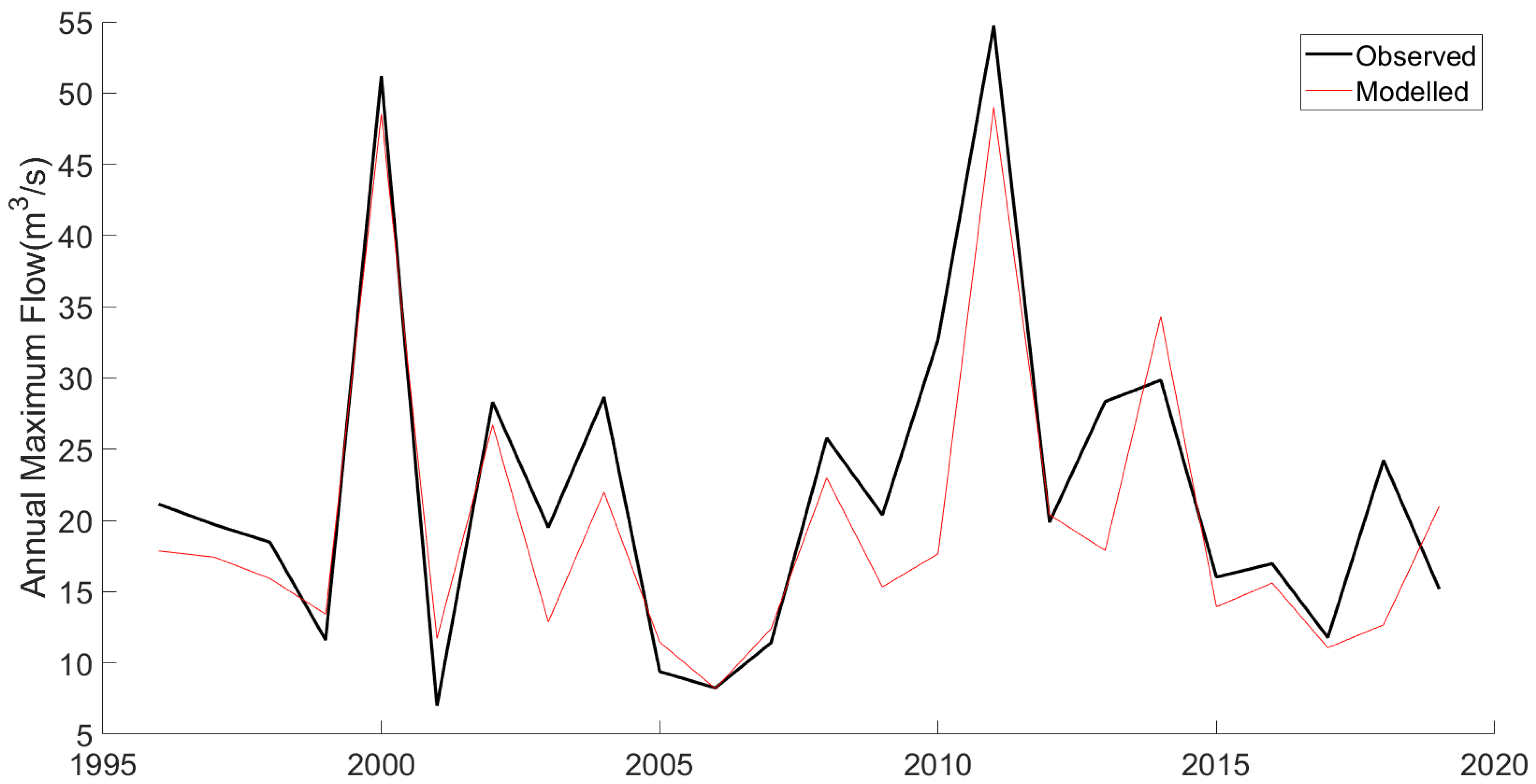
| Time Series | CORR | NSE | KGE |
|---|---|---|---|
| Daily | 0.776 | 0.548 | 0.713 |
| AMF | 0.905 | 0.772 | 0.815 |
| AMF Time Series | GEV Distribution Parameters | ||
|---|---|---|---|
| Historical | 16.534 | 8.535 | −0.017 |
| KNMI-4.5 | 15.926 | 9.747 | −0.025 |
| KNMI-8.5 | 18.491 | 9.983 | 0.043 |
| SMHI-4.5 | 16.156 | 5.819 | −0.202 |
| SMHI-8.5 | 18.877 | 8.709 | 0.183 |
| DMI-4.5 | 14.833 | 7.107 | −0.013 |
| DMI-8.5 | 12.625 | 9.651 | −0.083 |
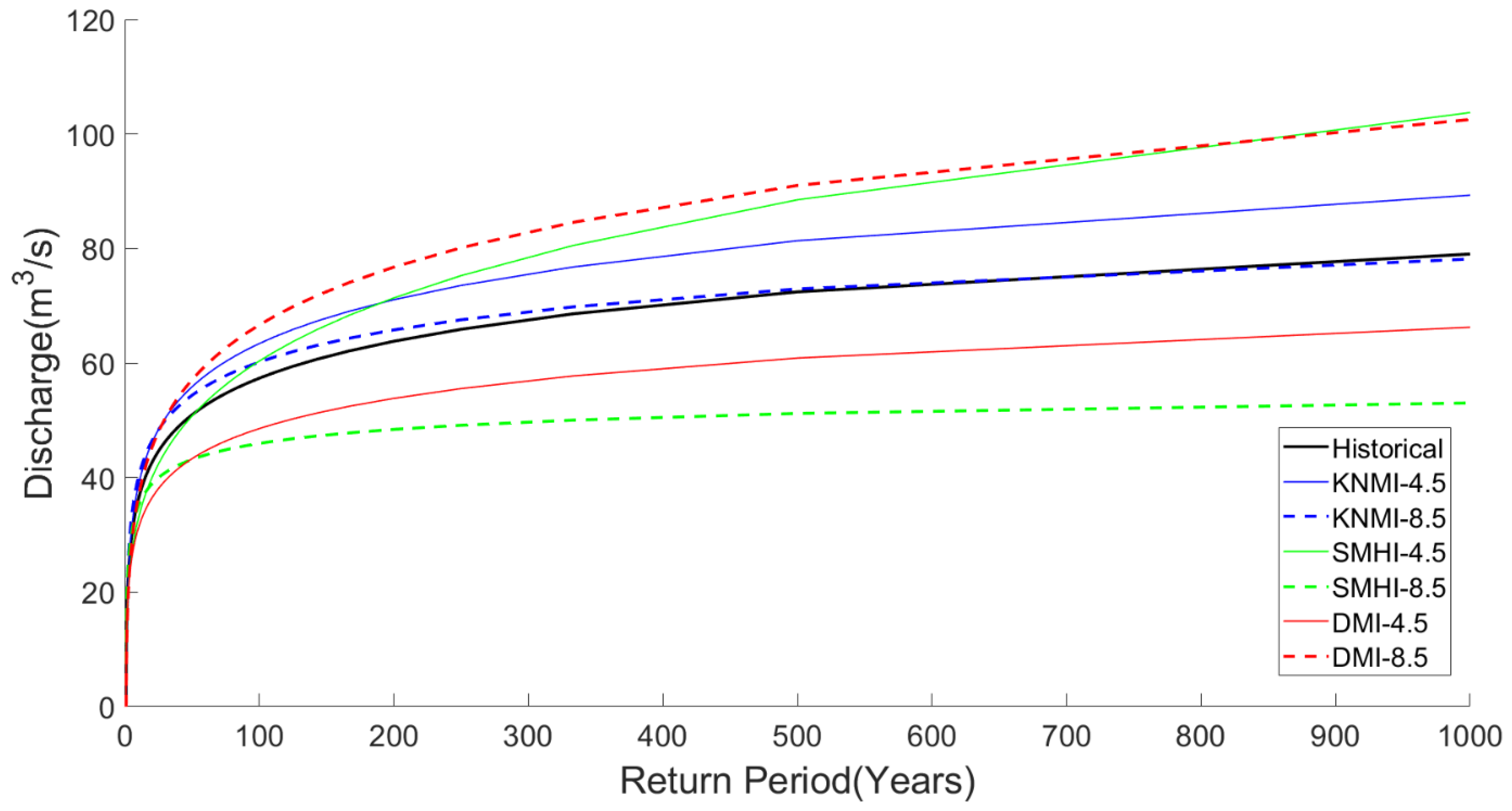
| AMF Time Series | Return Period (Years) | ||||
|---|---|---|---|---|---|
| 50 | 100 | 200 | 500 | 1000 | |
| Historical | 50.9 | 57.3 | 63.8 | 72.4 | 79.0 |
| KNMI-4.5 | 55.8 (9.6%) | 63.4 (10.6%) | 71.1 (11.4%) | 81.4 (12.3%) | 89.3 (13.0%) |
| KNMI-8.5 | 54.4 (6.7%) | 60.2 (4.9%) | 65.8 (3.1%) | 72.9 (0.7%) | 78.2 (−1.1%) |
| SMHI-4.5 | 50.7 (−0.4%) | 60.3 (5.2%) | 71.4 (11.9%) | 88.5 (22.2%) | 103.7 (31.3%) |
| SMHI-8.5 | 43.2 (−15.3%) | 46.0 (−19.9%) | 48.4 (−24.1%) | 51.2 (−29.3%) | 53.0 (−32.9%) |
| DMI-4.5 | 43.3 (−15.0%) | 48.5 (−15.3%) | 53.8 (−15.6%) | 60.9 (−16.0%) | 66.2 (−16.2%) |
| DMI-8.5 | 57.1 (12.0%) | 66.6 (16.2%) | 76.8 (20.3%) | 91.0 (25.7%) | 102.5 (29.7%) |
| Return Period (Years) | Flooded Area (km2) | Maximum Water Depth (m) | ||||||
|---|---|---|---|---|---|---|---|---|
| Historical | Future (DMI8.5) | Difference | % Increase | Historical | Future (DMI8.5) | Difference | % Increase | |
| 50 | 0.766 | 0.804 | 0.038 | 4.98 | 0.570 | 0.609 | 0.038 | 6.73 |
| 100 | 0.806 | 0.856 | 0.050 | 6.22 | 0.611 | 0.663 | 0.052 | 8.58 |
| 200 | 0.842 | 0.910 | 0.068 | 8.07 | 0.648 | 0.715 | 0.067 | 10.36 |
| 500 | 0.886 | 0.981 | 0.095 | 10.77 | 0.693 | 0.781 | 0.088 | 12.65 |
| 1000 | 0.923 | 1.045 | 0.122 | 13.27 | 0.726 | 0.866 | 0.140 | 19.32 |
Publisher’s Note: MDPI stays neutral with regard to jurisdictional claims in published maps and institutional affiliations. |
© 2022 by the authors. Licensee MDPI, Basel, Switzerland. This article is an open access article distributed under the terms and conditions of the Creative Commons Attribution (CC BY) license (https://creativecommons.org/licenses/by/4.0/).
Share and Cite
Sarkar Basu, A.; Gill, L.W.; Pilla, F.; Basu, B. Assessment of Climate Change Impact on the Annual Maximum Flood in an Urban River in Dublin, Ireland. Sustainability 2022, 14, 4670. https://doi.org/10.3390/su14084670
Sarkar Basu A, Gill LW, Pilla F, Basu B. Assessment of Climate Change Impact on the Annual Maximum Flood in an Urban River in Dublin, Ireland. Sustainability. 2022; 14(8):4670. https://doi.org/10.3390/su14084670
Chicago/Turabian StyleSarkar Basu, Arunima, Laurence William Gill, Francesco Pilla, and Bidroha Basu. 2022. "Assessment of Climate Change Impact on the Annual Maximum Flood in an Urban River in Dublin, Ireland" Sustainability 14, no. 8: 4670. https://doi.org/10.3390/su14084670
APA StyleSarkar Basu, A., Gill, L. W., Pilla, F., & Basu, B. (2022). Assessment of Climate Change Impact on the Annual Maximum Flood in an Urban River in Dublin, Ireland. Sustainability, 14(8), 4670. https://doi.org/10.3390/su14084670