
The Role of GARCH Effect on the Prediction of Air Pollution


Abstract
1. Introduction
2. Materials and Methods
2.1. Literature Review
2.2. Dataset
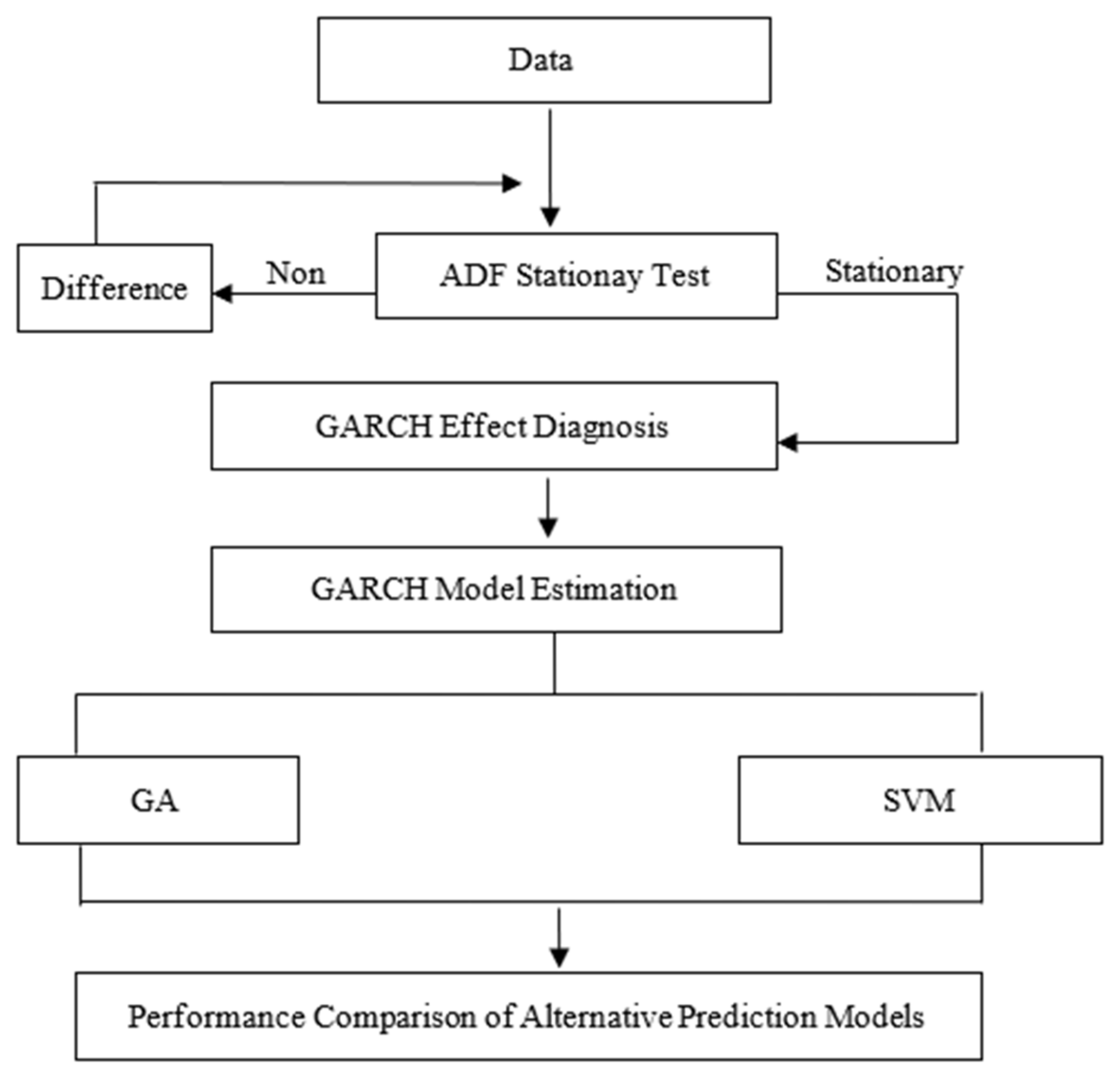
2.3. Methodology
2.3.1. Unit Root Test
- Model with neither intercept nor trend
- 2.
- Model with intercept but without trend
- 3.
- Model with both intercept and trend
2.3.2. ARCH Test
2.3.3. GARCH Model
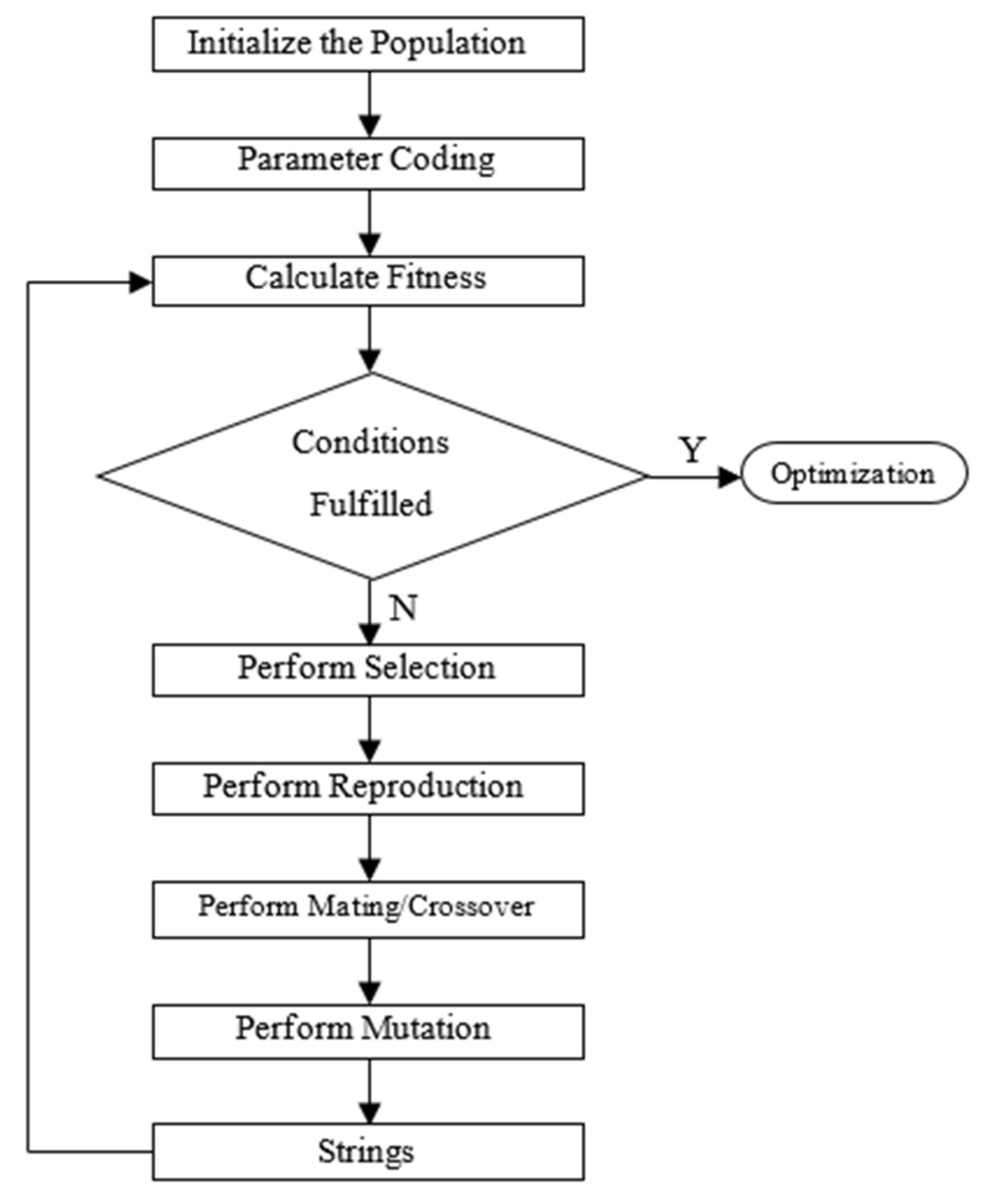
2.3.4. GA-SVM Model
2.3.5. Evaluation Indicators for Prediction Models
3. Results and Discussion
3.1. GARCH Effect Diagnosis
3.2. GARCH Estimation
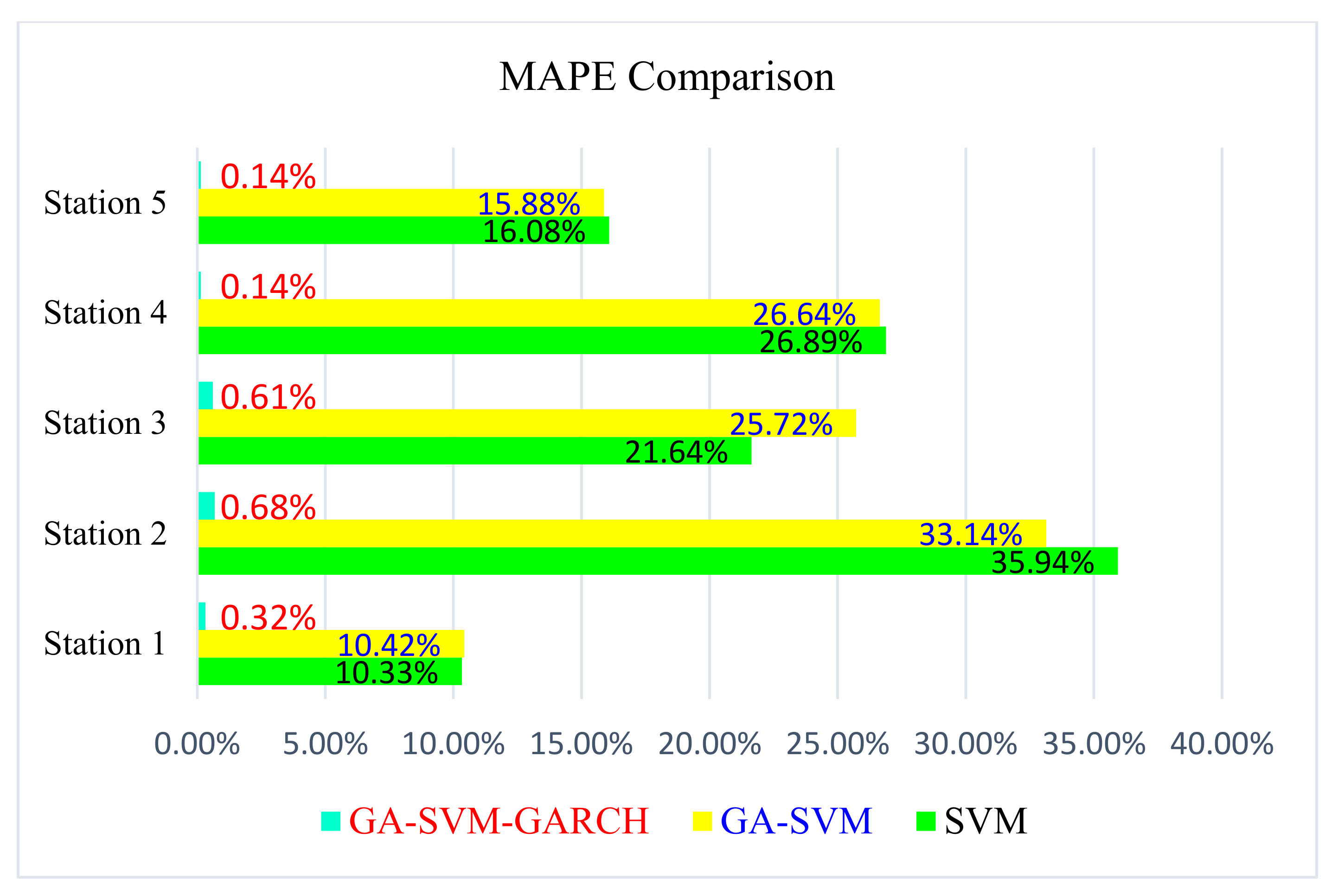
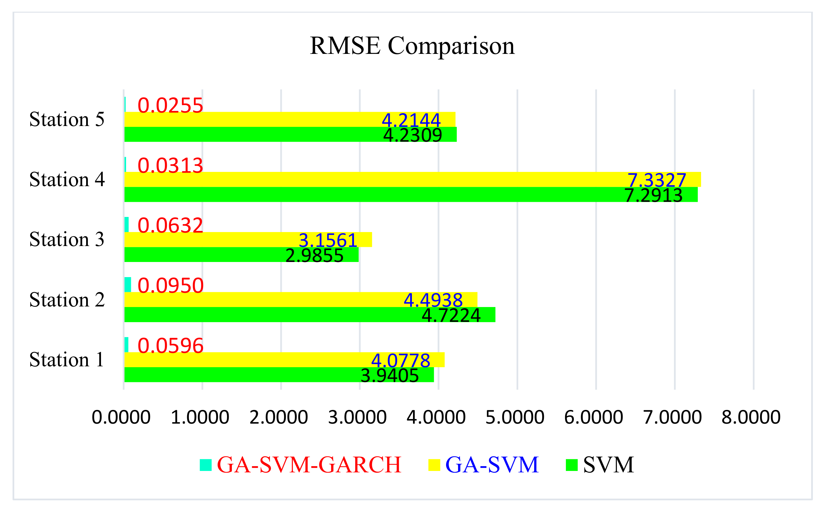
3.3. Evaluations of the Prediction Models
4. Conclusions
Author Contributions
Funding
Institutional Review Board Statement
Informed Consent Statement
Data Availability Statement
Acknowledgments
Conflicts of Interest
References
- Wikipedia. Air Pollution in Taiwan. Available online: https://en.wikipedia.org/wiki/Air_pollution_in_Taiwan (accessed on 27 February 2022).
- Chen, H.L.; Li, C.P.; Tang, C.S.; Lung, S.C.C.; Chuang, H.C.; Chou, D.W.; Chang, L.T. Risk assessment for people exposed to PM2.5 and constituents at different vertical heights in an urban area of Taiwan. Atmosphere 2020, 11, 1145. [Google Scholar] [CrossRef]
- Kusuma, W.L.; Wu, C.D.; Zeng, Y.T.; Hapsari, H.H.; Muhamad, J.L. PM2.5 pollutant in Asia—A comparison of metropolis cities in Indonesia and Taiwan. Int. J. Environ. Res. Public Health 2019, 16, 4924. [Google Scholar] [CrossRef] [PubMed]
- Xie, M.; Zhou, X. Taiwan Air Pollution Problem and Prevention Policy, National Policy Research Foundation. Available online: https://www.npf.org.tw/2/18414 (accessed on 27 February 2022).
- Long, Y.; Wang, J.; Wu, K.; Zhang, J. Population exposure to ambient PM2.5 at the subdistrict level in China. Int. J. Environ. Res. Public Health 2018, 15, 2683. [Google Scholar] [CrossRef] [PubMed]
- Chou, K.T. From anti-pollution to climate change risk movement: Reshaping civic epistemology. Sustainability 2015, 7, 14574–14596. [Google Scholar] [CrossRef]
- Feng, X.; Li, Q.; Zhu, Y.; Hou, J.; Jin, L.; Wang, J. Artificial neural networks forecasting of PM2.5 pollution using air mass trajectory based geographic model and wavelet transformation. Atmos. Environ. 2015, 107, 118–128. [Google Scholar] [CrossRef]
- Delavar, M.R.; Gholami, A.G.; Shiran, R.; Rashidi, Y.; Nakhaeizadeh, G.; Fedra, R.K.; Afshar, S.H. A novel method for improving air pollution prediction based on machine learning approaches: A case study applied to the capital city of Tehran. Int. J. Geo-Inf. 2019, 8, 99. [Google Scholar] [CrossRef]
- Engle, R.F. Autoregressive conditional heteroscedasticity with estimates of the variance of United Kingdom inflation. Econometrica 1982, 50, 987–1007. [Google Scholar] [CrossRef]
- Bollerslev, T. Generalized autoregressive conditional heteroscedasticity. J. Econom. 1986, 31, 307–327. [Google Scholar] [CrossRef]
- Hansen, P.R.; Lunde, A. A forecast comparison of volatility models: Does anything beat a garch(1,1)? J. Appl. Econom. 2005, 20, 873–889. [Google Scholar] [CrossRef]
- Zickus, M.; Greig, A.J.; Niranjan, M. Comparison of four machine learning methods for predicting PM10 concentrations in Helsinki, Finland. Water Air Soil Pollut. Focus 2002, 2, 717–729. [Google Scholar] [CrossRef]
- Dudot, A.L.; Rynkiewicz, J.; Steiner, F.E.; Rude, J. A 24-h forecast of ozone peaks and exceedance levels using neural classifiers and weather predictions. Environ. Model. Softw. 2007, 22, 1261–1269. [Google Scholar] [CrossRef]
- Voukantsis, D.; Karatzas, K.; Kukkonen, J.; Räsänen, T.; Karppinen, A.; Kolehmainen, M. Intercomparison of air quality data using principal component analysis, and forecasting of PM10 and PM2.5 concentrations using artificial neural networks, in Thessaloniki and Helsinki. Sci. Total Environ. 2011, 409, 1266–1276. [Google Scholar] [CrossRef] [PubMed]
- Russo, A.; Raischel, F.; Lind, P.G. Air quality prediction using optimal neural networks with stochastic variables. Atmos. Environ. 2013, 79, 822–830. [Google Scholar] [CrossRef]
- Tamas, W.; Notton, G.; Paoli, C.; Voyant, C.; Nivet, M.L.; Balu, A. Urban ozone concentration forecasting with artificial Neural Network in Corsica. Math. Model. Civil. Eng. 2014, 10, 29–37. [Google Scholar] [CrossRef][Green Version]
- Zhou, Q.; Jiang, H.; Wang, J.; Zhou, J. A hybrid model for PM2.5 forecasting based on ensemble empirical mode decomposition and a general regression neural network. Sci. Total Environ. 2014, 496, 264–274. [Google Scholar] [CrossRef] [PubMed]
- Elangasinghe, M.A.; Singhal, N.; Dirks, K.N.; Salmond, J.A.; Samarasinghe, S. Complex time series analysis of PM10 and PM2.5 for a coastal site using artificial neural network modelling and kmeans clustering. Atmos. Environ. 2014, 94, 106–116. [Google Scholar] [CrossRef]
- Kristiani, E.; Lin, H.; Lin, J.R.; Chuang, Y.H.; Huang, C.Y.; Yang, C.T. Short-term prediction of PM2.5 using LSTM deep learning methods. Sustainability 2022, 14, 2068. [Google Scholar] [CrossRef]
- Zheng, Y.; Yi, X.; Li, M.; Li, R.; Shan, Z.; Chang, E.; Li, T. Forecasting fine-grained air quality based on big data. In Proceedings of the 21st ACM SIGKDD International Conference on Knowledge Discovery and Data Mining, Sydney, Australia, 10–13 August 2015; pp. 2267–2276. [Google Scholar]
- Wang, T.; Jiang, F.; Deng, J.; Shen, Y.; Fu, Q.; Wang, Q.; Fu, Y.; Xu, J.; Zhang, D. Urban air quality and regional haze weather forecast for Yangtze River Delta region. Atmos. Environ. 2012, 58, 70–83. [Google Scholar] [CrossRef]
- Saide, P.E.; Mena-Carrasco, M.; Tolvett, S.; Hernandez, P.; Carmichael, G.R. Air quality forecasting for winter-time PM2.5 episodes occurring in multiple cities in central and southern Chile. J. Geophys. Res. Atmos. 2016, 121, 558–575. [Google Scholar] [CrossRef]
- Hu, K.; Sivaraman, V.; Bhrugubanda, H.; Kang, S.; Rahman, A. SVR based dense air pollution estimation model using static and wireless sensor network. In Proceedings of the 2016 IEEE Sensors, Orlando, FL, USA, 30 October–3 November 2016; pp. 1–3. [Google Scholar] [CrossRef]
- Davis, J.M.; Speckman, P. A model for predicting maximum and 8 hr average ozone in Houston. Atmos. Environ. 1999, 33, 2487–2500. [Google Scholar] [CrossRef]
- Siwek, K.; Osowski, S.; Garanty, K.; Sowinski, M. Ensemble of predictors for forecasting the PM10 pollution. In Proceedings of the VXV International Symposium on Theoretical Engineering, Lübeck, Germany, 22–24 June 2009; pp. 1–5. [Google Scholar]
- Sotomayor-Olmedo, A.; Aceves-Fernandez, M.A.; Gorrostieta-Hurtado, E.; Pedraza-Ortega, C.; Ramos-Arreguin, J.M.; Vargas-Soto, J.E. Forecast urban air pollution in Mexico City by using support vector machines: A kernel performance approach. Int. J. Intell. Sci. 2013, 3, 126–135. [Google Scholar] [CrossRef]
- Song, Z.; Niu, D.; Xiao, X.; Wu, H. Daily peak load forecasting based on fast k-medoids clustering, GARCH error correction and SVM model. J. Appl. Sci. Eng. 2016, 19, 249–258. [Google Scholar]
- Ishak, A.B.; Daoud, M.B.; Trabelsi, A. Ozone concentration forecasting using statistical learning approaches. J. Mater. Environ. Sci. 2017, 8, 4532–4543. [Google Scholar]
- Lin, K.M.; Chang, Y.S.; Zeng, Y.R.; Huang, C.X. Air pollution forecasting using machine learning methods on big data platform. In Proceedings of the TANET—Taiwan Academic NETwork Conference, Taoyuan, Taiwan, 20–24 October 2018; pp. 740–745. [Google Scholar]
- Granger, C.W.J.; Newbold, P. Spurious regressions in econometrics. J. Econom. 1974, 2, 111–120. [Google Scholar] [CrossRef]
- Engle, R.F.; Granger, C.W.J. Co-integration and error correction: Representation, estimation and testing. Econometrica 1987, 55, 251–276. [Google Scholar] [CrossRef]
- Christoffersen, P.F.; Diebold, F.X. Further results on forecasting and model selection under asymmetric loss. J. Appl. Econom. 1996, 11, 561–571. [Google Scholar] [CrossRef]
- Gerlach, R.; Chen, C.W.S.; Lin, D.S.Y.; Huang, M.H. Asymmetric responses of international stock markets to trading. Phys. A Stat. Mech. Its Appl. 2006, 360, 422–444. [Google Scholar] [CrossRef]
- Holland, J.H. Adaptation in Natural and Artificial Systems; The University of Michigan Press: Ann Arbor, MI, USA, 1975. [Google Scholar]
- Goldberg, D.E.; Korb, B.; Deb, K. Messy genetic algorithms: Motivation, analysis, and first results. Complex Syst. 1989, 3, 493–530. [Google Scholar]
- Shin, K.S.; Lee, Y.J. A genetic algorithm application in bankruptcy prediction modeling. Expert Syst. Appl. 2002, 23, 321–328. [Google Scholar] [CrossRef]
- Vapnik, V. Estimation of Dependences Based on Empirical Data; Springer Science & Business Media: Berlin/Heidelberg, Germany, 2006; pp. 430–438. [Google Scholar]
- Witten, I.H.; Mark, E.F.; Hall, A. Data Mining: Practical Machine Learning Tools and Techniques, 3rd ed.; Morgan Kaufmann: Burlington, MA, USA, 2011; p. 180. [Google Scholar]
- Lewis, C.D. Industrial and Business Forecasting Methods; Butterworths: London, UK, 1982; p. 40. [Google Scholar]


| Station 1 | Station 2 | Station 3 | Station 4 | Station 5 | |
|---|---|---|---|---|---|
| Location | FongYen | SaLu | DaLi | ChungMin | SeaTun |
| Duration | 58 days | 58 days | 58 days | 58 days | 58 days |
| Frequency | Hourly | Hourly | Hourly | Hourly | Hourly |
| Observations | 1211 | 1211 | 1215 | 1211 | 1211 |
| Mean absolute percentage error (MAPE) | |
| Root mean squared error (RMSE) | |
| Mean absolute error (MAE) | |
| Correlation coefficient (C. C.) | Here, is the mean value over the test data. |
| MAPE | Intepretation |
|---|---|
| MAPE < 10% | Highly accurate forecasting |
| 10% <MAPE < 20% | Good forecasting |
| 20% <MAPE < 50% | Reasonable forecasting |
| 50% <MAPE | Inaccuracte forecasting |
| Variable | Station 1 | Station 2 | Station 3 | Station 4 | Station 5 |
|---|---|---|---|---|---|
| PM2.5 (t−1) | 0.5408 | 0.5828 | 0.4945 | 0.5563 | 0.5543 |
| 25.80 *** | 31.70 *** | 24.83 *** | 30.10 *** | 28.47 *** | |
| CO | −0.9842 | 0.5406 | −0.1548 | −0.2233 | 0.9440 |
| −1.94 | 1.14 | −0.47 | −0.51 | 1.70 | |
| NO | 1.2822 | −0.0410 | −0.0046 | 0.2324 | 0.2220 |
| 1.55 | −0.56 | −0.01 | 0.47 | 0.34 | |
| NO2 | 1.2568 | 0.1181 | −0.1277 | 0.2902 | 0.1788 |
| 1.54 | 2.19 ** | −0.23 | 0.59 | 0.27 | |
| NOX | −1.0688 | −0.0139 | 0.1713 | −0.2036 | −0.1715 |
| −1.31 | −0.31 | 0.30 | −0.42 | −0.26 | |
| O3 | −0.0102 | 0.0090 | 0.0068 | 0.0030 | 0.0016 |
| −0.82 | 0.75 | 0.51 | 0.25 | 0.13 | |
| PM10 | 0.1547 | 0.1734 | 0.1970 | 0.1927 | 0.1801 |
| 13.28 *** | 16.86 *** | 18.01 *** | 17.60 *** | 16.73 *** | |
| SO2 | 0.4612 | 0.5779 | 0.6934 | 0.5627 | 0.3856 |
| 9.84 *** | 9.84 *** | 11.05 *** | 8.72 *** | 6.07 *** | |
| WindDirection | 0.0004 | 0.0012 | 0.0019 | −0.0003 | −0.0026 |
| 0.30 | 1.30 | 1.82 | −0.42 | −2.52 ** | |
| WindSpeed | 0.3763 | −0.1501 | −0.0007 | −0.4826 | −0.5618 |
| −2.15 ** | −1.86* | −0.09 | −3.14 *** | −5.11 *** | |
| C | 0.8794 | −1.3351 | −1.2469 | −0.1998 | 2.0251 |
| 1.71 * | −2.75 *** | −3.56 *** | −0.39 | 3.43 *** | |
| Observation | 1211 | 1211 | 1215 | 1211 | 1211 |
| F-statistic | 423.2258 | 739.5768 | 710.4244 | 740.6729 | 602.5055 |
| Prob. (F-stat.) | 0.0000 | 0.0000 | 0.0000 | 0.0000 | 0.0000 |
| Adj. R2 | 0.7773 | 0.8592 | 0.8532 | 0.8594 | 0.8325 |
| LM Test | |||||
| F-statistic | 16.2423 | 20.4623 | 21.2019 | 21.6132 | 20.8101 |
| Prob. (F-stat.) | 0.0000 | 0.0000 | 0.0000 | 0.0000 | 0.0000 |
| Obs*R2 | 31.9702 | 40.0022 | 41.4075 | 42.17369 | 40.6592 |
| Prob. (Chi2) | 0.0000 | 0.0000 | 0.0000 | 0.0000 | 0.0000 |
| ARCH test | |||||
| F-statistic | 231.4378 | 24.6600 | 31.1825 | 96.8117 | 148.2826 |
| Prob. (F-stat.) | 0.0000 | 0.0000 | 0.0000 | 0.0000 | 0.0000 |
| Obs*R2 | 194.5480 | 24.2067 | 30.4505 | 89.7771 | 132.2895 |
| Prob. (Chi2) | 0.0000 | 0.0000 | 0.0000 | 0.0000 | 0.0000 |
| Variable | Station 1 | Station 2 | Station 3 | Station 4 | Station 5 |
|---|---|---|---|---|---|
| GARCH (1,1) | |||||
| PM2.5 (t−1) | 0.5210 | 0.5528 | 0.4402 | 0.5577 | 0.4786 |
| 27.31 *** | 33.80 *** | 31.17 *** | 41.47 *** | 28.22 *** | |
| CO | 2.9016 | 2.4174 | 0.5319 | 2.5439 | 3.3907 |
| 6.28 *** | 8.16 *** | 1.47 | 9.13 *** | 5.75 *** | |
| NO | 0.9557 | −0.0513 | 0.6952 | 0.1474 | 0.1618 |
| 1.38 | −0.34 | 2.68 *** | 0.36 | 0.21 | |
| NO2 | 1.0488 | 0.0779 | 0.5710 | 0.1766 | 0.1172 |
| 1.53 | 0.53 | 2.24 ** | 0.44 | 0.16 | |
| NOx | −0.9170 | −0.0024 | −0.5645 | −0.1312 | -0.1266 |
| −1.33 | −0.02 | −2.21 ** | −0.32 | -0.17 | |
| O3 | −0.0025 | −0.0064 | −0.0153 | 0.0064 | 0.0060 |
| −0.28 | −0.64 | −1.26 | 0.75 | 0.58 | |
| PM10 | 0.1634 | 0.1635 | 0.2327 | 0.1755 | 0.2001 |
| 18.24 *** | 26.84 *** | 31.04 *** | 29.07 *** | 26.42 *** | |
| SO2 | 0.2115 | 0.5537 | 0.6148 | 0.2355 | 0.2485 |
| 5.64 *** | 16.23 *** | 9.04 *** | 5.42 *** | 3.71 *** | |
| WindDirection | −0.0012 | −0.0006 | −0.0001 | −0.0002 | −0.0024 |
| −1.28 | −0.95 | −0.10 | −0.28 | −3.40 *** | |
| WindSpeed | −0.3804 | −0.2110 | 0.0008 | −0.2507 | −0.4646 |
| −2.73 *** | −3.40 *** | 0.07 | −2.02 ** | −5.44 *** | |
| C | 1.1559 | −0.6811 | −0.4225 | −0.0385 | 1.8648 |
| 2.76 *** | −1.66 * | −1.69 * | −0.10 | 4.10 *** | |
| Variance Equation | |||||
| 2.8001 | 0.5845 | 7.1652 | 1.3838 | 0.9128 | |
| C | 7.03 *** | 6.24 *** | 9.53 *** | 5.47 *** | 4.01 *** |
| 0.3133 | 0.1689 | 0.4319 | 0.2426 | 0.1741 | |
| ε2(t−1) | 8.81 *** | 8.53 *** | 10.44 *** | 8.46 *** | 10.03 *** |
| 0.5639 | 0.8122 | 0.2937 | 0.6820 | 0.7891 | |
| h(t−1) | 14.08 *** | 44.93 *** | 5.72 *** | 20.11 *** | 35.78 *** |
| Model | Station 1 | Station 2 | Station 3 | Station 4 | Station 5 |
|---|---|---|---|---|---|
| SVM | |||||
| MAPE | 10.33% | 35.94% | 21.64% | 26.89% | 16.08% |
| RMSE | 3.9405 | 4.7224 | 2.9855 | 7.2913 | 4.2309 |
| GA-SVM | |||||
| MAPE | 10.42% | 33.14% | 25.72% | 26.64% | 15.88% |
| RMSE | 4.0778 | 4.4938 | 3.1561 | 7.3327 | 4.2144 |
| GA-SVM-GARCH | |||||
| MAPE | 0.32% | 0.68% | 0.61% | 0.14% | 0.14% |
| RMSE | 0.0596 | 0.0950 | 0.0632 | 0.0313 | 0.0255 |
Publisher’s Note: MDPI stays neutral with regard to jurisdictional claims in published maps and institutional affiliations. |
© 2022 by the authors. Licensee MDPI, Basel, Switzerland. This article is an open access article distributed under the terms and conditions of the Creative Commons Attribution (CC BY) license (https://creativecommons.org/licenses/by/4.0/).
Share and Cite
Yao, K.-C.; Hsueh, H.-W.; Huang, M.-H.; Wu, T.-C. The Role of GARCH Effect on the Prediction of Air Pollution. Sustainability 2022, 14, 4459. https://doi.org/10.3390/su14084459
Yao K-C, Hsueh H-W, Huang M-H, Wu T-C. The Role of GARCH Effect on the Prediction of Air Pollution. Sustainability. 2022; 14(8):4459. https://doi.org/10.3390/su14084459
Chicago/Turabian StyleYao, Kai-Chao, Hsiu-Wen Hsueh, Ming-Hsiang Huang, and Tsung-Che Wu. 2022. "The Role of GARCH Effect on the Prediction of Air Pollution" Sustainability 14, no. 8: 4459. https://doi.org/10.3390/su14084459
APA StyleYao, K.-C., Hsueh, H.-W., Huang, M.-H., & Wu, T.-C. (2022). The Role of GARCH Effect on the Prediction of Air Pollution. Sustainability, 14(8), 4459. https://doi.org/10.3390/su14084459