Article

Modeling of Land Use and Land Cover (LULC) Change Based on Artificial Neural Networks for the Chapecó River Ecological Corridor, Santa Catarina/Brazil

by
Juliana Mio de Souza
1,2,*,
Paulo Morgado
3,
Eduarda Marques da Costa
3 and
Luiz Fernando de Novaes Vianna
1
1
Agricultural Research and Extension Service Institution of the State of Santa Catarina, Rua Admar Gonzaga, 1347, Itacorubi, Florianópolis 88034-901, Brazil
2
Centre of Geographical Studies, Institute of Geography and Spatial Planning, University of Lisbon, Rua Branca Edmée Marques, 1600-276 Lisbon, Portugal
3
Centre of Geographical Studies, Associated Laboratory TERRA, Institute of Geography and Spatial Planning, University of Lisbon, Rua Branca Edmée Marques, 1600-276 Lisbon, Portugal
*
Author to whom correspondence should be addressed.
Sustainability 2022, 14(7), 4038; https://doi.org/10.3390/su14074038
Submission received: 25 February 2022 / Revised: 24 March 2022 / Accepted: 25 March 2022 / Published: 29 March 2022
(This article belongs to the Section Environmental Sustainability and Applications)

Abstract

:
The simulation and analysis of future land use and land cover—LULC scenarios using artificial neural networks (ANN)—has been applied in the last 25 years, producing information for environmental and territorial policy making and implementation. LULC changes have impacts on many levels, e.g., climate change, biodiversity and ecosystem services, soil quality, which, in turn, have implications for the landscape. Therefore, it is fundamental that planning is informed by scientific evidence. The objective of this work was to develop a geographic model to identify the main patterns of LULC transitions between the years 2000 and 2018, to simulate a baseline scenario for the year 2036, and to assess the effectiveness of the Chapecó River ecological corridor (an area created by State Decree No. 2.957/2010), regarding the recovery and conservation of forest remnants and natural fields. The results indicate that the forest remnants have tended to recover their area, systematically replacing silviculture areas. However, natural fields (grassland) are expected to disappear in the near future if proper measures are not taken to protect this ecosystem. If the current agricultural advance pattern is maintained, only 0.5% of natural fields will remain in the ecological corridor by 2036. This LULC trend exposes the low effectiveness of the ecological corridor (EC) in protecting and restoring this vital ecosystem.

1. Introduction

Land use and land cover change (LULC) occurs due to human activities and natural processes [1,2,3,4]. Currently, regardless of whether the impacts of change are positive or negative, they are mostly driven to meet human needs [5]. LULC changes can significantly affect some core aspects of how the Earth’s system works, such as biodiversity, soil quality and ecosystem carrying capacity [5,6].
The conceptual difference between land use and land cover is functional. While land cover is classified according to “what is physically on” the land surface (natural or otherwise), land use refers to the activities carried out on a given portion of the territory [7,8,9,10,11]. In this research, both terms are presented in a combined form: land use and land cover (LULC), since they are complementary and interrelated terms as substantiated by the literature [12].
LULC dynamics are characterized by their complexity, which involves a set of interactions between biophysical and socioeconomic processes [5,6]. Modeling is a tool that allows us to understand the causes and consequences of LULC dynamics and analyze scenarios to support land use planning [13].
Artificial intelligence (AI), as an analytical method, has had an increasingly important role in our society in almost every field [14,15,16,17,18], including among the territory analysis methods [19,20,21]. Different groups of AI systems use different algorithms and are suitable for different purposes [22]. LULC dynamics can be typically modeled by methods that have various implementation complexities and efficiencies [23], such as Markov chains (MC) [24,25,26,27], cellular automata (CA) [28,29,30,31,32], and artificial neural networks (ANN) [19,20,33,34,35,36,37,38]. Its applications are suitable for urban [20,28,34,39] and rural [19,26,35,40,41] environments and it can be applied to different settings. LULC dynamics often result from a complex inter-system combination of factors, a non-trivial collective behavior, that cannot be derived from an individual or a simple collection of systemic analyses. We adopted the ANN method for LULC prediction because previous empirical studies comparing neural networks and more traditional learning methods often find better forecasting results in the former [34]. Furthermore, neural networks offer fault-tolerant solutions and they can better learn from and make decisions based on incomplete, noisy, and fuzzy information [42]. Moreover, we used the MLP type of ANN, which is one the most popular ANN supervised techniques currently used due to the robustness of the results [43,44].
Historically, land use and land cover dynamics in Brazil have two main drivers—urbanization and the growth of the primary sector (agriculture, livestock and extractivism) [45,46,47,48,49,50,51]. While urbanization is responsible for the gradual and intense replacement of natural environments by urban agglomerations, primary activities use extensive areas but maintain a minimum of soil permeability and vegetation cover, even if not perennial. In the state of Santa Catarina, a close relationship can be observed between the growth of farming and silviculture and land use and land cover changes [52]. The constant growth of the gross value of production (GVP) of the state’s mixed farming reflects this dynamic and is also an important economic indicator [53]. This context of socioeconomic growth versus LULC changes reveals the importance of using LULC change analysis and simulation methods to support the development and assessment of public policies.
The assessment of LULC changes proposed in this paper aims to identify transition patterns between LULC classes at a more detailed level of observation than is typically performed in studies using only the transition matrix as the method of analysis [26,54]. The method is based on computing the persistence of LULC classes while identifying the most significant changes. By computing the persistence of LULC classes, it is possible to extract the maximum knowledge about the potential processes that determine a given LULC change pattern. Through persistence, it is possible to assess LULC changes in terms of the area that has changed, the dynamics of change between the various classes, and the spatial pattern of change. This method allows scientists and managers to focus on the strongest signals of systematic landscape transitions, ultimately necessary to link a pattern and process [54].
The purpose of this research was to develop a simulation and analysis model of LULC change trends for the year 2036, based on artificial neural networks (ANN) and in inter-class systematic transition patterns proposed by Pontius et al. (2004) [54] in the Chapecó River ecological corridor (EC), in order to provide a robust tool to support decision-making, land use planning and sustainable development. ANN-MLP is a machine learning data-driven method. The accuracy and robustness of its outcomes derive from training optimization functions that fine-tune the learning process and minimize prediction error [55]. It is recommended, for model robustness purposes, that the number of prediction years should not be greater than the time interval between model input data [19,20,34,55], which in our case are 18 years (from 2000 to 2018). That being said, we can adopt a one-size-fits-all approach ANN type of model, because each dataset requires a tailored approach for the sake of the model soundness. For each step of the study, the specific objectives were: to select the physical, social, economic and environmental variables that could potentially influence LULC dynamics; to parameterize and validate the LULC dynamics simulation model for the year 2036; to identify LULC changes between the years 2000–2018 (observed) and 2018–2036 (simulated), and to assess the effectiveness of the creation of the ecological corridor as an environmental preservation/conservation public policy tool.
This paper is organized as follows: Section 2 presents the description of the study area, the used data, and the methodology adopted. Section 3 presents the results and discussions about the main systematic transitions of LULC and the effectiveness of the ecological corridor as a policy for conservation and environmental restoration. Finally, Section 4 presents the main findings of the research and implications of the method, presenting the main conclusions of the research.

2. Materials and Methods
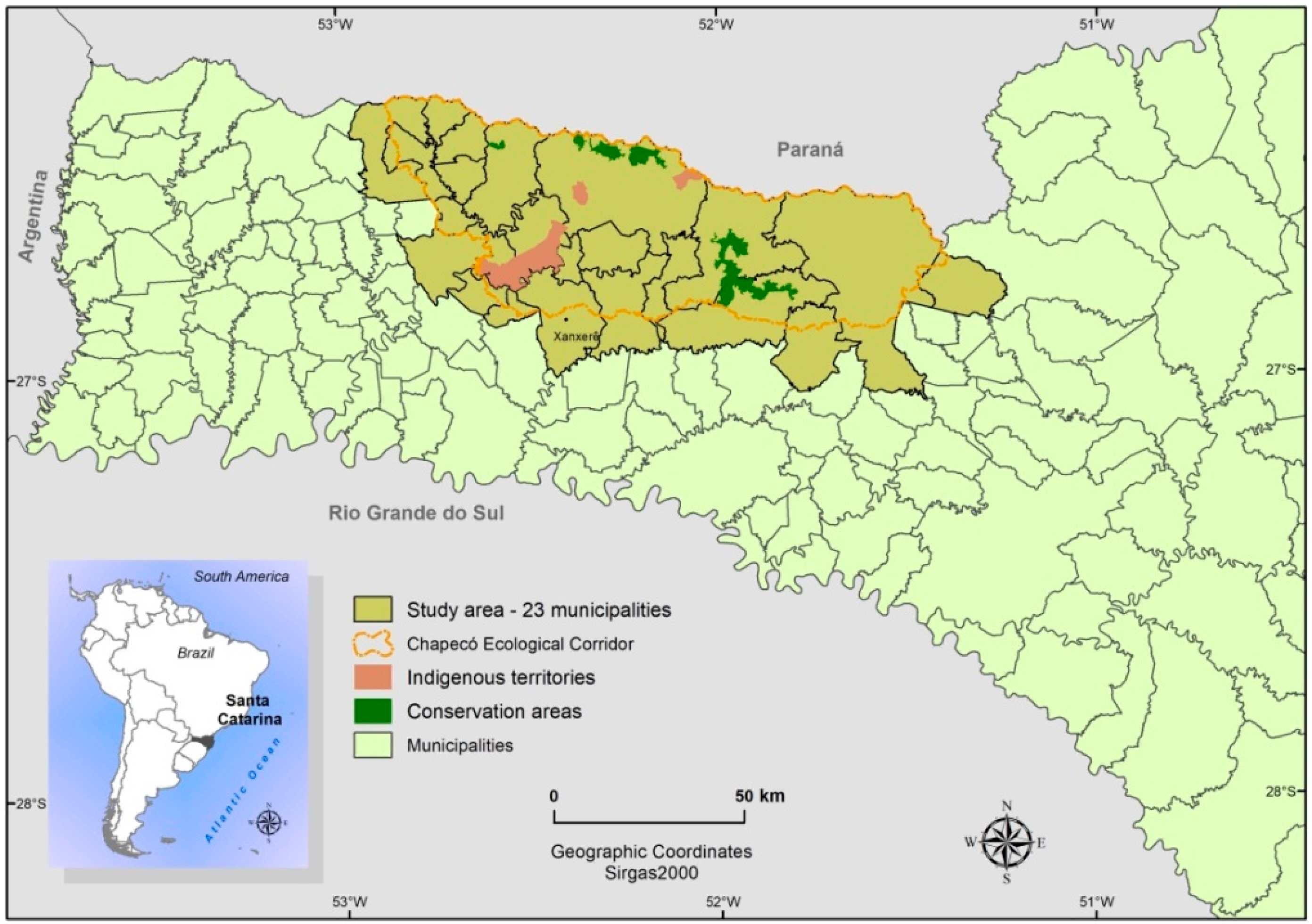
2.1. Study Area

The study area is located northwest of the state of Santa Catarina, in the southern region of Brazil (Figure 1). It has an approximate area of 7242 km2 and is located between the geographic coordinates 27°5′0″ and 26°20′0″ south latitude and 53°0′0″ and 51°10′0″ west longitude. It is delimited by the political boundaries of the 23 municipalities that make up the Chapecó River ecological corridor (Chapecó EC). The Chapecó EC was created by the State of Santa Catarina/Brazil Government through the State Decree, No. 2957 of 20 January 2010 [56]. It was designed due to the need to preserve biodiversity in essential remnants of the Atlantic Forest biome and associated natural ecosystems [56]. Its main objective is to “develop and implement a model to enhance, market and leverage native forests (and other natural environments) as environmental assets, promoting the maintenance and improvement of landscape permeability” [57,58].
The Chapecó EC displays a high complexity of social arrangements. It houses 37 agrarian reform settlements (family farmers and settlers), 3 indigenous lands, and 3 conservation units (2 federal and 1 state) (Figure 1). The main economic activities are soybean cultivation, beef, and dairy cattle raising, and timber production [58].
The study area occupies approximately 7% of the total area of the state of Santa Catarina, where 185,116 inhabitants live (2.62% of the state’s population) [61]. Among the 23 municipalities that make up the study area, Xanxerê stands out, with just over 50,000 inhabitants [62]. The other municipalities are considered small-sized (less than 50 thousand inhabitants). The study area has an agricultural and livestock tradition, with an average demographic density of 28.2 inhabitants per km2, lower than the state’s average (99.7 inhabitants per km2), and an urbanization rate of 49.4% [61]. The municipalities that make up the study area contribute 2.2% of the state GDP (6.2 million in 2017), and their household income per capita is 30% lower than the state average income [61].
In 2018, there were 67.9 thousand people formally employed, of which 35% were in the manufacturing sector, followed by the service sector (21.6%) and trade (18.5%) [63]. The main industrial segment is food products manufacturing, which, together with the sectors of pulp, paper and paper products manufacturing and wood products manufacturing, accounted for more than 75% of the formally employed workforce [63].
Regarding natural characteristics, the study area is part of the Atlantic forest biome and has a natural patchwork of vegetation types, composed of mixed ombrophilous forest (araucaria forest), deciduous seasonal forest, and gramineous and hardwood steppe (natural fields) [58,64]. Geomorphologically, it is formed by the Campos Gerais Plateau and the Dissected Plateau. On the Campos Gerais Plateau, the altimetric levels vary between 800 m and 1200 m and are higher than the surrounding areas of the Dissected Plateau unit. The latter makes a tremendous topographic contrast with the areas of the Campos Gerais Plateau, with its strongly dissected relief formed by deep valleys and terraced slopes. The main soil types found in the Chapecó EC are latosols, nitosols, cambisols and litholic soils, where cambisol is the predominant soil type [65,66,67].
As for the type of climate, according to Koeppen’s classification, in areas below 800 m, the climate is of the humid mesothermal type with hot summers (Cfa), where the remnants of the deciduous seasonal forest are found. In areas above this altitude, the climate is humid mesothermal with cool summers (Cfb), where the natural fields and the mixed ombrophilous forest are. The average annual temperature ranges from 15 °C to 18 °C [68], with well-distributed rainfall throughout the year, varying between 1640 mm and 2035 mm [67,68].
According to MapBiomas mapping [69], in 2018, the LULC agriculture class covered 33.36% of the study area. The forest class covered 28.96%, while pasture and silviculture occupied just over 12% each. The grassland class accounted for 2.06% of the study area, and artificial areas and water bodies combined accounted for less than 1% of the total area.
To represent the Chapecó EC through its physical, social and economic aspects and simulate a LULC scenario for 2036, a method based on ANN was applied [5,34,70,71], whose steps were: (i) data issues; (ii) parameterization of the LULC model; (iii) validation of the LULC model; (iv) analysis of LULC changes between the observed period (2000–2018) and the simulated period (2018–2036); and (v) the assessment of the effectiveness of the Chapecó EC as a LULC management tool.

2.2. Modeling LULC Change

Figure 2 illustrates a procedural and methodological flowchart of the activities involved in developing the model. The keys indicate the four specific objectives that make up the proposed main goal. The processes resulting from the boxes in key 1 resulted in the systematization of a set of 37 variables selected due to their potential explanatory factor of LULC changes in the study area. This is the input for modeling LULC changes. Key 2 illustrates the processes performed for modeling the LULC changes for the Chapecó EC under an artificial neural network approach. This step resulted in the simulation of LULC changes for the year 2036 for the study area. The third key is the LULC change analyses for the observed and simulated periods. This step of model building is intended to identify the most significant patterns of change (which is ultimately necessary to link the pattern to the process [54]), and the fourth key was an analysis of the effectiveness of the Chapecó EC as an environmental management tool, assessing the changes that have occurred and the trends of changes in the classes involving, mainly, the Atlantic forest remnants and the natural fields.

2.3. Data Issues

The choice of variables in LULC change studies should be based on the knowledge of the forces that cause change and create dynamics in a specific territory. These forces and the variables that represent them can be social, economic, demographic/population, environmental, political, and cultural (driving forces) [5,34,70,71].
The selection of representative data for the variables implies the adoption of two main criteria: 1—the existence of spatial representation at a scale compatible with the analysis throughout the study area, and 2—the existence of a temporal history consistent with the period studied with at least two representative dates [21].
Table 1 shows the metadata of the data sources used. The variables used in the model match those commonly adopted in LULC simulations [19,20,34,35,72], and the raw data used were obtained from various sources, with different formats and temporal representations (Table 1).
The organization and systematization of this dataset were conducted in a GIS (Geographic Information System) environment, using ArcGis 10.7 [78] and IDRISI Selva [79]. The representative data of each variable were converted to a raster format, with a 100-m spatial resolution, and referenced to the SIRGAS2000 system, Universal Transverse Mercator projection (UTM 22S). The choice of spatial resolution was based on the relation between computer processing time and the minimum scale of the data, without prejudice to the intended analyses regarding LULC dynamics [80]. We generated 68 rasters, equivalent to 37 variables multiplied by the number of corresponding years (Table 1). As an example, for the LULC data from MapBiomas, two rasters were generated, one for the year 2000 and another for 2018.
Table 2 presents the relationship of the variables (driving forces) used in the ANN-based LULC change simulation model and their analysis dimensions. The data represent a total of 37 variables, where 6 are from the physical dimension, 20 economic, 6 social, 3 technological, and 2 demographic. The analysis dimension makes up the forces that cause change and creates dynamics in the territory (physical, social, economic, demographic, and technological/political dimensions) [5,6,70,81,82].
The physical/natural dimension describes some of the study area’s natural, physical and weather characteristics. In the economic dimension, there are variables that depict the road infrastructure of the study area, agricultural production (herd size, yield and value), employment and income distribution, and land value. The social dimension deals with the social arrangements and socioeconomic development. The technological dimension includes some variables used to measure the technological level employed in rural properties. Finally, there is the population dimension (general and rural).

LULC Class Nomenclature Definition

According to the MapBiomas project, nine LULC classes were originally presented in the study area: forest formation, forest plantation, grassland, pasture, annual and perennial crop, mosaic of agriculture and pasture, urban infrastructure, other non-vegetated area, and river, lake and ocean [69]. For this research, the nomenclature of the classes was modified. Urban infrastructure and other non-vegetated area were grouped together and termed artificial areas. Table 3 presents the nomenclature of the classes changed according to the LULC descriptions defined by the classification key adopted in the MapBiomas project [69] and the phytogeographic typologies of Santa Catarina [64].

2.4. Parameterization of the LULC Simulation Model

To model LULC changes, the type of machine learning adopted was ANN, based on the multilayer perceptron (MLP) network and the backpropagation algorithm. This is the most widely used model conformation in this type of work [19,20,22,34,35,83,84,85]. Eight models named ANN1 to ANN8 were constructed (Table 3), based on experimentation with different parameterizations [16,20,34,86,87], and IBM SPSS 24 was used [88]. The input layer data, hidden layer activation function, and output layer data and parameters have been kept constant in all eight models. The difference between the models was the parameterization of the number of cases for the sample partitions for network training, testing and validation; the number of hidden layers; the number of hidden layer neurons; and the number of iterations (Table 4).

2.5. Validation of the Model

The validation of the model was based on the area under the curve (AUC) measurement, derived from the relative operating characteristic, also known as the receiver operating characteristic (ROC) [89]. The AUC value lets us know how well the model can distinguish between the classes [35,90,91,92]. The higher the value, the better the ability of the model to differentiate the classes. AUC values are between 0 and 1, where 0.5 indicates that the model is unable to distinguish between the classes, and 1 corresponds to a perfect fit [29,45,46] AUC values between 0.7 and 0.8 are considered acceptable, values between 0.8 and 0.9 are considered very good, and values above 0.9 are considered excellent [93].

2.6. Analysis of LULC Changes

The space–time analysis of LULC changes was based on the LULC class area for 2000, 2018, and 2036. Complementing this analysis, the method proposed by Pontius et al. [54] and applied by Viana and Rocha [26] was adopted. From the calculation of the transition matrix (cross-tabulation) between the LULC maps for the years 2000 and 2018 (observed period), and 2018 and 2036 (simulated period), the behavior of each class and the transitions between classes were verified.
The transition matrix presents, on its diagonal, the persistence for each LULC class (Pjj) from the initial time (T1) to the final time (T2). The column total, P+j, denotes the landscape proportion of each LULC class at the final time, and the row total, Pj+, is the proportion of each LULC class at the initial time. The off-diagonal values represent the transitions between classes from the initial to the final time. In addition to persistence, for each class, eight more metrics were calculated: gain, loss, total change, swap, net change [26,54], tendency to gain rather than lose, tendency to lose rather than persist, tendency to gain rather than persist [26]. Table 5 shows the description of each metric used in the LULC change analysis.
To analyze the transitions between classes and identify whether those transitions were random or systematic, the method of comparing expected and observed LULC values was applied [54].
To this end, six new LULC change matrices were generated, three for a gain situation and three for an area loss situation between classes, containing: (i) the expected area percentage of each class if the changes occurred randomly; (ii) the difference between the observed area percentage and the expected area percentage for each class—this difference defines the fingerprint left on the landscape (subtraction method); (iii) the ratio between the fingerprint and the expected percentage area for each class, which highlights the strength of the transition and provides values that indicate a systematic, or otherwise, transition process between LULC classes. The details of the equations used to generate the matrices can be seen in [26,54].

2.7. Assessment of the Effectiveness of the Chapecó River EC as a Public Policy

To assess the effectiveness of the Chapecó River ecological corridor as an environmental management public policy tool, the legal instruments that define the mechanisms of direct or indirect action on LULC’s changing dynamics were considered. Article 2 of Decree No. 2957 of January 2010 [56] sets out an objective of the ecological corridor I—“to preserve the remnants of the mixed ombrophilous forest (forest) and southern fields from economic mechanisms, based on the valorization of regional vocations and the region’s natural resources.” The Chapecó River EC management plan [58] identifies as primary threats to LULC, a change in the expansion of silviculture (planting exotic trees); agriculture in areas of natural fields; and deforestation (forest).
In order to assess the effectiveness of the conservation of the remnants of the mixed ombrophilous forest and the natural fields (southern fields) and to verify the power of the response to the threats and the objective of the creation of the ecological corridor, the metrics that describe the transition process of the forest, silviculture, agriculture and grassland classes were used.

3. Results and Discussions

3.1. Model Validation and LULC Simulation for 2036

The results of the ANN model’s performance and network training time are presented in Table 6. The complete results for the “rounds” of the eight parameterized models are available in the Supplementary Materials for this article (S1: Model ANN-MLP).
The model that met the pre-established performance criteria was the ANN1 model, with the highest cross-entropy value. The hit percentage, when predicting LULC classes, was similar for every model. The network training time was the second-fastest, and the processing time was half the time that the models with two hidden layers took (ANN5 to ANN8). To determine the accuracy of the ANN1 model, the area under the ROC curve was used [94]. The curves numbered 1 to 8 correspond to the following LULC classes: forest (1), silviculture (2), grassland (3), pasture (4), agriculture (5), mosaic (6), artificial area (7), and water bodies (8) (Figure 3).
All LULC classes presented values higher than 0.7, demonstrating that the model has high separability and accuracy among the different land use and land cover classes. These results are consistent with other ANN-based LULC simulation studies [34,35,81]. The model showed excellent accuracy in the forest, grassland, agriculture, artificial area and water bodies classes (>90%). The silviculture and pasture classes, with a value between 80% and 90%, were classified as “very good,” and only the mosaic class was classified as “acceptable” (79.4%).
The mosaic class is composed of two classes: agriculture and pasture, which may explain the higher degree of uncertainty in its classification in a machine learning and simulation process. According to the accuracy studies of the MapBiomas project volume 4.1, this class presented an approximately 35% inclusion error [69]. Another characteristic of this class that may explain its lower hit rate, is its sparse spatial distribution and surrounding larger patches of other LULC classes (Figure 4).
Thus, the ANN1 model was considered fit to simulate LULC changes between 2018 and 2036 (Figure 4c).

3.2. LULC Changes

3.2.1. Spatial and Temporal Evolution of Land Use and Land Cover

The spatial and temporal evolution of LULC in the study area, which occurred between the years 2000 and 2018, and the evolution trends for the year 2036 can be observed in the maps of Figure 4. Table 7 shows the areas of the LULC map classes for each evaluated year.
In 2000 and 2018, the forest class was predominant, covering 33.39% and 28.96% of the study area, respectively (Figure 4 and Table 6). However, from 2000 to 2018, there was a loss of 320 km2 of forest. According to the simulation result, under constant current conditions, this area may be recovered by 2036.
Between 2000 and 2018, the silviculture class increased from 4.46% of the total area to 12.62%—an increase of 190%. According to the simulation result, silviculture will again occupy close to 6% of the study area in 2036.
The agriculture class area grew between 2000 and 2018 and will keep on growing, according to the simulation for 2036. While between 2000 and 2018, it increased by 35%. According to the model, the agriculture class area is expected to grow by 9.1% in the 2018–2036 period.
In 2000, the grassland class already occupied a small area (4.8% of the total area) compared to the other LULC classes. From 2000 to 2018, it lost 55% of its area (in Brazil, the loss of this ecosystem in 32 years (1985 to 2017) was 9.8% [95]) and, according to the model, the trend indicates that only 0.47% of the study area will still be covered by grassland by 2036.
Despite different methodological approaches, these results corroborate with other studies of LULC change, where they identify trends of expansion of agricultural areas, such as agriculture and silviculture, and a loss of forest area in different regions of the country and the world (Latin America, Africa, South and Southeast Asia, and China) [5,19,45,46,47,48,49,50,52,70,71,95], and the marked loss of grassland area in the southern region of Brazil [95,96,97,98]. Trends of increasing forest area and loss and/or relative stagnation of areas dedicated to agriculture are perceived in different regions of the world [20,26,70,99].

3.2.2. LULC Changes and the Main Systematic Transitions Observed between the Years 2000 and 2018

The most significant transitions between classes in terms of area percentage between 2000 and 2018 were from pasture to agriculture (5.46%), from pasture to mosaic (4.17%), and from forest to silviculture (3.42%) (see Table 8). Ecologically, the transition between agricultural areas (pasture, agriculture, and mosaic) does not determine the loss of natural areas, but silviculture has proved to be an invasive activity in forests.
In addition to the forest and silviculture transition, which proved to be significant, the behavior of the agriculture and grassland classes has to be assessed, since these classes are related to the threats and the goal of the creation of the ecological corridor.
The transition matrix (Table 8) may induce a naïve analysis of the results, simply highlighting the most significant transitions, usually associated with the classes with more coverage in the study area. An example of this is the grassland class, which despite having lost 55% of its area in the analysis period (Table 7), does not stand out as one of the major transitions (Table 8).
In order to properly reveal the dynamic behaviors of LULC classes and transitions between classes, complementary metrics need to be considered. These metrics are calculated based on the transition matrix and depict the persistence, gain, loss, swap (associated with a place change), and net change (associated with quantity change) of each LULC class, and the systematic transitions, which are those that occur beyond what would be expected in a random change process.
As shown in Table 9, approximately 1/3 of the study area experienced LULC changes, and almost 70% of its area remained unchanged. In terms of total change, 16.33% was attributed to an exchange process (Sj) and 18.44% was attributed to net change (Dj). This means that the area’s change process was slightly higher (2.21%) than the place change process.
The dynamics of the forest class were marked by the loss of its area at a rate more than twice (7.54%) the area gain between 2000 and 2018. Furthermore, in terms of change, of the 10.66% total change of the forest class in the study area, more than half of that change is attributed to a pattern of place change (6.23%) rather than area change. As shown in Figure 5a, the loss of forest remnants is concentrated around areas dedicated to silviculture.
The silviculture class was marked by an area gain relative to the loss process, at a rate of 76.18% (G/L). This gain process occurred in the study area region where silviculture was already a prevalent activity, substantiated by the gain patches around the persistence patches (Figure 5b).
The agriculture class was marked by an area gain dynamics, where the gain represented almost four times the loss rate (3.77%). The most significant gains of the agriculture class were concentrated on the grassland areas and around persistence areas (Figure 5c). The grassland class (Figure 5d) stood out with an area loss of more than two times (Lp = 2.20%) compared to its persistence rate (Pj = 1.51%).
The information provided in Table 7 and Table 8 made it possible to quantify the net change of each class, besides the gain, loss and swaps, and to identify the major transitions between classes. However, to identify the most significant systematic transitions, Table 10 has to be analyzed.
If the transitions between classes occurred randomly in terms of both gain and loss, the “observed minus expected” metrics shown in Table 10 should be zero, but this is not the case. Moreover, the farther away from zero is the “difference divided by expected” ratio, the stronger the signal of a systematic transition.
In order to examine the main transitions, Table 10 presents those with the strongest change signals (positive and negative).
The transition between forest and silviculture shows a systematic transition pattern due to strong transition signals, especially regarding the transition process in terms of losses. When forest loses, this class is replaced by silviculture, marked by a fingerprint that represents a difference of 2.08% of the study area. Studies point to a transition trend due to economic pressure and market policies [45,49].
The transition between forest and agriculture shows a strong but negative signal of the transition between classes. This means that when agriculture gains, it does not replace forest, and when forest loses, it is not replaced by agriculture. The agriculture class gained less from the forest (3.50% of its area) than would be expected due to a random process of forest loss, and the forest class lost less to agriculture (1.80%) than would be expected due to a random process of agriculture gain.
Similarly, the transition between agriculture and grassland represents a systematic transition pattern. The expansion of agriculture over natural areas is evidenced in other studies [5,52,70], and specifically over grassland areas [100]. The most robust evidence of this systematic pattern is in the high signals of this transition in terms of gains. The strength of this transition is equivalent to a rate more than one and a half times what would be expected if the agriculture class gained randomly. A systematic pattern is evidenced where agriculture replaces grassland but does not replace the forest.
The result of Table 10 demonstrates that two of the major transitions between classes that were pointed out directly in the transition matrix (Table 7), also stand out as major systematic transitions (forest to silviculture and pasture to mosaic). The grassland to agriculture transition, albeit not one of the major transitions evidenced in the transition matrix of Table 7, was characterized as one of the most significant systematic transitions occurring in the study area, according to the complementary analyses of LULC dynamics presented. This result reveals the importance of analyzing the dynamics of LULC considering random and systematic transitions [26,54,100].

3.2.3. LULC Changes and the Main Simulated Systematic Transitions for the Year 2036

The most significant transitions between classes expected to occur between 2018 and 2036 will be between agriculture and pasture (3.59%), silviculture and forest (3.42%), mosaic and pasture (3.20%), and pasture and agriculture (3.19%). The transitions between agricultural classes (pasture, mosaic and agriculture) are significant in terms of area but do not determine any loss of natural area.
Although the simulation model (2036) indicates a 55% loss of the grassland class area (Table 7), the transition pattern of this class is not highlighted by the transition matrix as one of the key transitions (Table 11), just as it was not highlighted in the observed 2000–2018 period.
As it has been done for the observed period (2000–2018), the same metrics were calculated based on the transition matrix for the simulation period (2018–2036) to analyze LULC changes and identify key systematic transitions.
The results in Table 12 indicate that, according to the LULC simulation model for 2036, 32.9% of the total change is expected to occur in the study area, with approximately 20% of that change tending towards swapping patterns, i.e., place change.
According to Table 12, the forest class will experience an increase in area since it tends to gain area rather than lose it at a rate of about two and a half times, as shown by the G/L metric. A change in this class will be marked by a swapping pattern, corresponding to 6.23% of the total expected change (10.66%). Figure 6a shows that the forest class tends to gain more area around the patches where this class persists and in areas previously dedicated to silviculture.
Change in the silviculture class will be marked by a pattern of area loss, as shown by the metrics Lj and Lp (Table 12 and Figure 6b). The Lj metric indicates that the likelihood of the silviculture class losing area is more than seven times greater than that class gaining area. Likewise, the Lp metric indicates that silviculture is more likely to be lost than to be maintained (1.42%).
The agriculture class will present the most significant area persistence, with 26.5% of its class (Table 12 and Figure 6c). By 2036, agriculture will keep on expanding as shown by the gain metric (9.92%), higher than the loss metric (6.86%). Figure 6c illustrates a higher concentration of agricultural area gain in grassland. Another characteristic of the agriculture class is that it will respond to a swapping pattern, corresponding to 13.72% of the total change of 16.78% expected for 2036.
The grassland class (Figure 6d) stood out due to an area loss of more than ten times (Lp = 10.09%) compared to its persistence rate (Pj = 0.19%).
The information provided in Table 11 and Table 12 made it possible to quantify the net change of each class, in addition to the gain, loss, swaps, and to identify the main transitions between classes that will occur in the simulated 2018–2036 period. Similarly, to what was done for the observed period, to identify the most significant systematic transitions, we need to analyze the results of the transitions in Table 13.
Table 13 shows the transitions that indicated the strongest change signals (positive and negative) for the simulated period (2036).
According to the results shown in Table 13, the silviculture to forest transition tends to behave as a systematic transition—even though, in case of loss, the replacement of the silviculture class by the forest class shows a weak signal. The tendency to transition from silviculture to forest may be related to the current slowdown in the silviculture market, as shown in other studies [101].
When the agriculture class gains area, it does not replace forest, as shown by the negative sign (−3.44%). When a forest loses area, it is not replaced by agriculture in a random process of loss of the forest class.
The grassland class will change systematically to the agriculture class since when the agriculture class gains area, it tends to gain it from the grassland class at a rate of almost four times what would be expected if the agriculture class gains were random. Similarly, when grassland loses area, it loses it to the agriculture class (0.79%) and (1.15%).
The transition between mosaic and pasture classes stands out due to the strong transition signals. When the pasture class gains area, it tends to gain it from the mosaic class—2.04% of its area. Conversely, when the mosaic class loses area, it tends to lose it to the pasture class (1.78%).
Of the four key transitions identified in the transition matrix in Table 10, two of them, the transitions from mosaic to pasture and silviculture to the forest, stand out and are confirmed as a trend of systematic transition patterns for the simulated period (2018–2036).
The grassland and agriculture transition were not evidenced as the major transition in the transition matrix (Table 11). However, it is one of the most significant systematic transitions identified for the simulated period, where, in terms of gains, it showed the highest (positive) conversion signals. This result reveals a probability of maintenance of the systematic transition of grassland into agriculture, with risks of significant loss of local biodiversity [96,97,102] and confirms the importance of elaborating future scenarios of LULC change to support decision making and territory management, aiming at environmental sustainability [19,34,55,80].

3.3. Effectiveness of the Chapecó River EC as an Environmental Management Tool

The Chapecó River EC was created in 2010, and the observed period of analyses of LULC changes was from 2000 to 2018. Therefore, for ten years of this period (2000–2010), this environmental management tool was not implemented in the study area.
The agricultural classes, indicated as threats, showed an expansion behavior in the study area, with a systematic pattern of replacement of natural areas. Silviculture expanded over forest remnants, and the loss of grassland resulted from the advance of agriculture.
For the observed period (2000–2018), there are clear indications that the protective measures were insufficient to respond positively to the threats or even reverse an established pattern of advancement of agricultural activities over natural areas.
For the simulated period (2036), the agriculture into grassland transition continues to be a trend, where grassland conversion into areas dedicated to agriculture will leave only 0.5% of this natural cover in the study area, showing little power to respond to one of the main threats presented in the Chapecó River EC management plan [58].
The loss of this ecosystem can have negative ecological, social, and economic consequences. The natural fields of the Atlantic forest are among the most biodiverse grasslands in the world and stand out as an essential ecosystem for biodiversity conservation, carbon storage and the maintenance of significant ecosystem services [96,97,102].
Regarding forest remnants, forest areas (mixed ombrophilous forest or araucaria forest) show a recovery trend, replacing silviculture areas. However, one cannot state that this forest recovery is due exclusively to the effectiveness of the public policy of the ecological corridor.
In the same period, there was a slowdown in silviculture in the state of Santa Catarina, which expanded its planted area by 116.31% between 2000 and 2010; while between 2010 and 2018, that expansion rate dropped to 21.89% [69]. The rural environmental land register (Cadastro Ambiental Rural—CAR) was also implemented [103]. This register is mandatory and ensures the environmental regularization and adequacy of rural properties in Brazil, constituting a requirement to obtain benefits and financing and participate in programs and authorizations. The CAR and the environmental regularization program (Programa de Regularização Ambiental—PRA) establishes a formal commitment by the rural landowner to maintain, recover or restore degraded areas or altered areas in permanent preservation areas, legally reserve and restrict the use of the rural property areas, or to compensate legal reserve areas.

4. Conclusions

The simulation of LULC dynamics being based on artificial neural networks (ANN), allowed us to project a future alternative and identify the main land use and land cover change trends for the Chapecó EC. The use of ANN to simulate LULC dynamics does not require a priori knowledge about the data and the local dynamics. However, modeling variables describing the region’s physical, social, economic, and environmental characteristics, and representing the driving forces of change in the territory can contribute to the machine learning capabilities. The model offered excellent accuracy in most classes. Using a higher complexity neural network parameterized with two hidden layers did not improve the accuracy of LULC class separability and doubled the network’s training time.
The transition matrix is a key feature to analyze LULC dynamics. However, to detect systematic LULC transitions, one must assess other metrics from the transition matrix, such as each class persistence and net change. Performing an analysis of LULC dynamics based solely on the most significant transitions presented by the transition matrix may lead the researcher or decision-makers to wrongful conclusions. The dynamics of the grassland class identified in this research is a case in point. The transition matrix did not reveal the transition from grassland to agriculture as one of the major transitions. However, the complementary analyses showed that, for both periods (observed and simulated), this transition between classes was the primary and most robust systematic transition in the landscape. Without this analysis, perhaps the systematic loss of one of the most important biomes in the study area would go unnoticed since, proportionally, its area is much smaller than the area of the other LULC classes.
The areas dedicated to agriculture remain the main drivers for the replacement of natural areas, especially natural fields. The expansion of the agricultural activity in the study area reflects a state policy guided by the foreign market, where agribusiness corresponds to 70.2% of the state’s total exports in 2020 [104]. Silviculture exhibits a systematic pattern of replacing forest areas in the observed period (2000–2018). However, according to the simulation, this pattern will be reversed, and forest areas systematically will replace the silviculture class.
Given this scenario, the creation of the Chapecó River EC as a conservation and environmental protection tool proved to be barely effective concerning the conservation of one of the most critical ecosystems in the state, the natural fields. Natural fields stand out as an important ecosystem for biodiversity conservation, carbon storage and the maintenance of significant ecosystem services [96,97,102]. The loss of this natural vegetation can have negative ecological, social, and economic consequences. New policies are needed to promote and support the restoration of degraded areas, maintain sustainable land practices, create conservation units, and include Brazil’s non-forest environments in the priority agenda for conservation and restoration [97].
As for the recovery trend of forest areas, there are positive indications of the effectiveness of the Chapecó EC as an environmental management tool. However, one cannot assert that this recovery occurred only due to the implementation of this management tool. Studies have to be complemented because other policies, such as the implementation of CAR, market issues (e.g., a slowdown in the silviculture market, with a reduction of approximately 10% of the planted area in the state between 2014 and 2020 [101]), and physical conditions (slope, relief, type of soil), may have contributed to the decrease in deforestation and forest recovery.

Supplementary Materials

The complete results for the “rounds” of the eight parameterized models are available online at https://www.mdpi.com/article/10.3390/su14074038/s1, Report S1: Model ANN-MLP.

Author Contributions

Conceptualization, J.M.d.S., P.M. and E.M.d.C.; methodology, J.M.d.S., P.M. and E.M.d.C.; software, J.M.d.S.; validation, J.M.d.S. and P.M.; formal analysis, J.M.d.S. and L.F.d.N.V.; investigation, J.M.d.S.; data curation, J.M.d.S.; writing—original draft preparation, J.M.d.S. and L.F.d.N.V.; writing—review and editing, J.M.d.S., P.M., E.M.d.C. and L.F.d.N.V. All authors have read and agreed to the published version of the manuscript.

Funding

This research received no external funding.

Acknowledgments

We would like to acknowledge Epagri—the Agricultural Research and Extension Service Institution of the State of Santa Catarina/Brazil for providing the opportunity for the first author to pursue her doctoral studies; and the Geomodlab—the Laboratory for Remote Sensing, Geographical Analysis and Modelling—of the Centre of Geographical Studies/IGOT for providing the required equipment, software, and the financial support for publishing this paper.

Conflicts of Interest

The authors declare no conflict of interest.

References

  1. Foley, J.A.; Ramankutty, N.; Brauman, K.A.; Cassidy, E.S.; Gerber, J.S.; Johnston, M.; Mueller, N.D.; O’Connell, C.; Ray, D.K.; West, P.C.; et al. Solutions for a cultivated planet. Nature 2011, 478, 337–342. [Google Scholar] [CrossRef] [Green Version]
  2. Lambin, E.F.; Turner, B.L.; Geist, H.J.; Agbola, S.B.; Angelsen, A.; Bruce, J.W.; Coomes, O.T.; Dirzo, R.; Fischer, G.; Folke, C.; et al. The causes of land-use and land-cover change: Moving beyond the myths. Glob. Environ. Chang. 2001, 11, 261–269. [Google Scholar] [CrossRef]
  3. Feranec, J.; Soukup, T.; Taff, G.N.; Stych, P.; Bicik, I. Overview of changes in land use and land cover in Eastern Europe. In Land-Cover and Land-Use Changes in Eastern Europe after the Collapse of the Soviet Union in 1991; Springer: Cham, Switzerland, 2016; pp. 13–33. ISBN 9783319426389. [Google Scholar]
  4. Fuchs, R.; Herold, M.; Verburg, P.H.; Clevers, J.G.P.W.; Eberle, J. Gross changes in reconstructions of historic land cover/use for Europe between 1900 and 2010. Glob. Chang. Biol. 2015, 21, 299–313. [Google Scholar] [CrossRef]
  5. Lambin, E.F.; Geist, H.; Rindfuss, R.R. Introduction: Local Processes with Global Impacts. In Land Use and Land Cover Change; Lambin, E.F., Geist, H., Eds.; Springer: Berlin/Heidelberg, Germany, 2006; pp. 1–8. ISBN 9783540322016. [Google Scholar]
  6. Geist, H.; McConnell, W.; Lambin, E.F.; Moran, E.; Alves, D.; Rudel, T. Causes and Trajectories of Land-Use/Cover Change. In Land-Use and Land-Cover Change; Lambin, E.F., Geist, H., Eds.; Springer: Berlin/Heidelberg, Germany, 2006; pp. 41–70. ISBN 978-3-540-32201-6. [Google Scholar]
  7. Martínez, S.; Mollicone, D. From Land Cover to Land Use: A Methodology to Assess Land Use from Remote Sensing Data. Remote Sens. 2012, 4, 1024–1045. [Google Scholar] [CrossRef] [Green Version]
  8. Briassoulis, H. Analysis of Land Use Change: Theoretical and Modeling Approaches; Regional Research Institute, WVU-West Virginia University: Morgantown, WV, USA, 2000. [Google Scholar]
  9. FAO. Planning for Sustainable Use of Land Resources: Towards a New Approach; Food and Agriculture Organisation: Rome, Italy, 1995; ISBN 9251037248. [Google Scholar]
  10. Turner, B., II; Skole, D.; Sanderson, S.; Fischer, G.; Fresco, L.; Leemans, R. Land-Use and Land-Cover Change Science/Research Plan; IGBP: Stockholm, Sweden; Geneva, Switzerland, 1995. [Google Scholar]
  11. Quan, B.; Chen, J.-F.; Qiu, H.-L.; Römkens, M.J.M.; Yang, X.-Q.; Jiang, S.-F.; Li, B.-C. Spatial-Temporal Pattern and Driving Forces of Land Use Changes in Xiamen. Pedosphere 2006, 16, 477–488. [Google Scholar] [CrossRef]
  12. Fisher, P.; Comber, A.; Wadsworth, R. Land use and land cover: Contradiction or complement. In Re-Presenting GIS; Fisher, P., Unwin, D.J., Eds.; John Wiley & Sons Ltd.: New York, NY, USA, 2005; ISBN 9780470848470. [Google Scholar]
  13. Verburg, P.H.; Schot, P.P.; Dijst, M.J.; Veldkamp, A. Land use change modelling: Current practice and research priorities. GeoJournal 2004, 61, 309–324. [Google Scholar] [CrossRef]
  14. Liu, J.; Tang, Z.H.; Zeng, F.; Li, Z.; Zhou, L. Artificial neural network models for prediction of cardiovascular autonomic dysfunction in general Chinese population. BMC Med. Inform. Decis. Mak. 2013, 13, 1–7. [Google Scholar] [CrossRef] [Green Version]
  15. Ahmed, F.E. Artificial neural networks for diagnosis and survival prediction in colon cancer. Mol. Cancer 2005, 4, 1–12. [Google Scholar] [CrossRef] [Green Version]
  16. Pianucci, M.N. Uma Proposta para a Obtenção da População Sintética Através de Dados Agregados para Modelagem de Geração de Viagens por Domicílio. Ph.D. Thesis, Universidade de São Paulo, scola de Engenharia de São Carlos, Butanta, Brazil, 2016. [Google Scholar]
  17. Le, L.T.; Nguyen, H.; Dou, J.; Zhou, J. A comparative study of PSO-ANN, GA-ANN, ICA-ANN, and ABC-ANN in estimating the heating load of buildings’ energy efficiency for smart city planning. Appl. Sci. 2019, 9, 2630. [Google Scholar] [CrossRef] [Green Version]
  18. Ghadami, N.; Gheibi, M.; Kian, Z.; Faramarz, M.G.; Naghedi, R.; Eftekhari, M.; Fathollahi-Fard, A.M.; Dulebenets, M.A.; Tian, G. Implementation of solar energy in smart cities using an integration of artificial neural network, photovoltaic system and classical Delphi methods. Sustain. Cities Soc. 2021, 74, 103149. [Google Scholar] [CrossRef]
  19. Padilha, D.G. Modelo de Apoio à Decisão Aplicado ao Planejamento Territorial de Silvicultura Baseado em Análise Multicritério de Redes Neurais Artificiais. Ph.D. Thesis, Universidade Federal de Santa Maria, Santa Maria, Brazil, 2014. [Google Scholar]
  20. Gomes, E.; Abrantes, P.; Banos, A.; Rocha, J.; Buxton, M. Farming under urban pressure: Farmers’ land use and land cover change intentions. Appl. Geogr. 2019, 102, 58–70. [Google Scholar] [CrossRef]
  21. Gomes, E.; Banos, A.; Abrantes, P.; Rocha, J.; Kristensen, S.B.P.; Busck, A. Agricultural land fragmentation analysis in a peri-urban context: From the past into the future. Ecol. Indic. 2019, 97, 380–388. [Google Scholar] [CrossRef]
  22. Faceli, K.; Lorena, A.C.; Gama, J.; Carvalho, A.C.P.L.F. Inteligência Artificial: Uma Abordagem de Aprendizado de Máquina; LTC: Rio de Janeiro, Brazil, 2011; ISBN 8521618808. [Google Scholar]
  23. Agarwal, C.; Green, G.M.; Grove, J.M.; Evans, T.P.; Schweik, C.M. A Review and Assessment of Land-Use Change Models: Dynamics of Space, Time, and Human Choice. Apollo Int. Mag. Art Antiq. 2002, 62. [Google Scholar] [CrossRef] [Green Version]
  24. Hathout, S. The use of GIS for monitoring and predicting urban growth in East and West St Paul, Winnipeg, Manitoba, Canada. J. Environ. Manag. 2002, 66, 229–238. [Google Scholar] [CrossRef]
  25. Weng, Q. Land use change analysis in the Zhujiang Delta of China using satellite remote sensing, GIS and stochastic modelling. J. Environ. Manag. 2002, 64, 273–284. [Google Scholar] [CrossRef] [Green Version]
  26. Viana, C.M.; Rocha, J. Evaluating dominant land use/land cover changes and predicting future scenario in a rural region using a memoryless stochastic method. Sustainability 2020, 12, 4332. [Google Scholar] [CrossRef]
  27. Anand, J.; Gosain, A.K.; Khosa, R. Prediction of land use changes based on Land Change Modeler and attribution of changes in the water balance of Ganga basin to land use change using the SWAT model. Sci. Total Environ. 2018, 644, 503–519. [Google Scholar] [CrossRef]
  28. Da Silva Pinto, F.J.P. Sistemas Complexos, Modelação e Geosimulação da Evolução de Padrões de Uso e Ocupação do Solo. Ph.D. Thesis, Universidade de Lisboa, Instituo de Geografia e Ordenamento do Território, Lisbon, Portugal, 2012. [Google Scholar]
  29. Yirsaw, E.; Wu, W.; Shi, X.; Temesgen, H.; Bekele, B. Land Use/Land Cover change modeling and the prediction of subsequent changes in ecosystem service values in a coastal area of China, the Su-Xi-Chang region. Sustainability 2017, 9, 1204. [Google Scholar] [CrossRef] [Green Version]
  30. Liu, Y.; Feng, Y. Simulating the impact of economic and environmental strategies on future urban growth scenarios in Ningbo, China. Sustainability 2016, 8, 1045. [Google Scholar] [CrossRef] [Green Version]
  31. Hamad, R.; Balzter, H.; Kolo, K. Predicting land use/land cover changes using a CA-Markov model under two different scenarios. Sustainability 2018, 10, 3421. [Google Scholar] [CrossRef] [Green Version]
  32. Sinha, S.; Sharma, L.K.; Nathawat, M.S. Improved Land-use/Land-cover classification of semi-arid deciduous forest landscape using thermal remote sensing. Egypt. J. Remote Sens. Space Sci. 2015, 18, 217–233. [Google Scholar] [CrossRef] [Green Version]
  33. Li, X.; Yeh, A.G.O. Neural-network-based cellular automata for simulating multiple land use changes using GIS. Int. J. Geogr. Inf. Sci. 2002, 16, 323–343. [Google Scholar] [CrossRef]
  34. Morgado, P.; Gomes, E.; Costa, N. Competing visions? Simulating alternative coastal futures using a GIS-ANN web application. Ocean Coast. Manag. 2014, 101, 79–88. [Google Scholar] [CrossRef]
  35. Silva, L.P.; Xavier, A.P.C.; da Silva, R.M.; Santos, C.A.G. Modeling land cover change based on an artificial neural network for a semiarid river basin in northeastern Brazil. Glob. Ecol. Conserv. 2020, 21, e00811. [Google Scholar] [CrossRef]
  36. Azari, M.; Tayyebi, A.; Helbich, M.; Reveshty, M.A. Integrating cellular automata, artificial neural network, and fuzzy set theory to simulate threatened orchards: Application to Maragheh, Iran. GIScience Remote Sens. 2016, 53, 183–205. [Google Scholar] [CrossRef]
  37. Naushad, R.; Kaur, T.; Ghaderpour, E. Deep Transfer Learning for Land Use and Land Cover Classification: A Comparative Study. Sensors 2021, 21, 8083. [Google Scholar] [CrossRef]
  38. Solórzano, J.V.; Mas, J.F.; Gao, Y.; Gallardo-Cruz, J.A. Land use land cover classification with U-net: Advantages of combining sentinel-1 and sentinel-2 imagery. Remote Sens. 2021, 13, 3600. [Google Scholar] [CrossRef]
  39. Megahed, Y.; Cabral, P.; Silva, J.; Caetano, M. Land cover mapping analysis and urban growth modelling using remote sensing techniques in greater Cairo region-Egypt. ISPRS Int. J. Geo-Inf. 2015, 4, 1750–1769. [Google Scholar] [CrossRef] [Green Version]
  40. Lira, P.K.; Tambosi, L.R.; Ewers, R.M.; Metzger, J.P. Land-use and land-cover change in Atlantic Forest landscapes. For. Ecol. Manag. 2012, 278, 80–89. [Google Scholar] [CrossRef]
  41. Martínez-Vega, J.; Díaz, A.; Nava, J.M.; Gallardo, M.; Echavarría, P. Assessing land use-cover changes and modelling change scenarios in two mountain Spanish national parks. Environments 2017, 4, 79. [Google Scholar] [CrossRef] [Green Version]
  42. Fischer, M. Computational neural networks-tools for spatial data analysis. In Spatial Analysis and GeoComputation: Selected Essays; Springer: Berlin/Heidelberg, Germany, 2006; pp. 79–102. ISBN 3540357297. [Google Scholar]
  43. Fischer, M. Expert systems. In Spatial Analysis and GeoComputation: Selected Essays; Springer: Berlin/Heidelberg, Germany, 2006; pp. 61–76. ISBN 3540357297. [Google Scholar]
  44. Mather, P.M.; Openshaw, S.; Openshaw, C. Artificial Intelligence in Geography. Geogr. J. 1998, 164, 353. [Google Scholar] [CrossRef]
  45. Defries, R.S.; Rudel, T.; Uriarte, M.; Hansen, M. Deforestation driven by urban population growth and agricultural trade in the twenty-first century. Nat. Geosci. 2010, 3, 178–181. [Google Scholar] [CrossRef]
  46. Yoshikawa, S.; Sanga-Ngoie, K. Deforestation dynamics in Mato Grosso in the southern Brazilian Amazon using GIS and NOAA/AVHRR data. Int. J. Remote Sens. 2011, 32, 523–544. [Google Scholar] [CrossRef]
  47. Silva, J.; Abdon, M.; Silva, S.; Moraes, J. Evolution of deforestation in the brazilian pantanal and surroundings in the timeframe 1976–2008. Geografia 2011, 36, 35–55. [Google Scholar]
  48. Asner, G.P. Automated mapping of tropical deforestation and forest degradation: CLASlite. J. Appl. Remote Sens. 2009, 3, 33543. [Google Scholar] [CrossRef]
  49. Lipp-Nissinen, K.H.; De Sá Piñeiro, B.; Miranda, L.S.; De Paula Alves, A. Temporal dynamics of land use and cover in Paurá Lagoon region, Middle Coast of Rio Grande do Sul (RS), Brazil. J. Integr. Coast. Zone Manag. 2018, 18, 25–35. [Google Scholar] [CrossRef] [Green Version]
  50. Silva, E.A.; Ferreira, R.L.C.; da Silva, J.A.A.; Sá, I.B.; Duarte, S.M.A. Dinâmica do uso e coberura da tarra do município de Floresta, PE. Embrapa Semiárido-Artig. Periódico Indexado 2013, 43, 611. [Google Scholar] [CrossRef] [Green Version]
  51. Rodrigues, L.P.; Leite, E.F. Dinâmica do uso e cobertura da terra na bacia hidrográfica do rio Aquidauana, MS. Os Desafios da Geografia Física na Fronteira do Conhecimento 2017, 1, 6817–6825. [Google Scholar] [CrossRef] [Green Version]
  52. Souza, J.M.; Costa, E.M. Methodological proposal to analyze land use and land cover changes: The case of Santa Catarina state in Brazil from 2000 to 2010. Sustentabilidade em Debate 2020, 11, 485–517. [Google Scholar] [CrossRef]
  53. Epagri/Cepa. Síntese Anual da Agricultura de Santa Catarina; Epagri: Florianópolis, Brazil, 2019; p. 197. [Google Scholar]
  54. Pontius, R.G.; Shusas, E.; McEachern, M. Detecting important categorical land changes while accounting for persistence. Agric. Ecosyst. Environ. 2004, 101, 251–268. [Google Scholar] [CrossRef]
  55. Peponi, A.; Morgado, P.; Trindade, J. Combining Artificial Neural Networks and GIS Fundamentals for Coastal Erosion Prediction Modeling. Sustainability 2019, 11, 975. [Google Scholar] [CrossRef] [Green Version]
  56. Santa Catarina. Decreto no 2.957, de 20 de janeiro de 2010; Gov. do Estado St. Catarina: Florianópolis, Brazil, 2010. [Google Scholar]
  57. Zuchiwschi, E. Fatores de Influência na Conservação e Manejo de Florestas Nativas em Unidades de Produção Agrícolas do Corredor Ecológico Chapecó; Universidade Federal de Santa Catarina: Santa Catarina, Brazil, 2013. [Google Scholar]
  58. Socioambiental. Plano de Gestão do Corredor Ecológico Chapecó, Santa Catarina. Relatório Técnico; Socioambiental Consult; Assoc. e Fundação do Meio Ambient: Florianópolis, Brazil, 2009; p. 130. [Google Scholar]
  59. Secretaria de Estado do Planejamento: Diretoria de Geografia e Cartografia. Mapa Político de Santa Catarina—1:500,000. 2013. Available online: http://arcgis.ciram.sc.gov.br:6080/arcgis/rest/services/ESTACOES_METEO/Estudo_OMM_Estacoes/MapServer/5 (accessed on 1 August 2020).
  60. ArcWorld Supplement. Esri Data & Maps Media Kit. World Continents—1:15,000,000. Available online: https://www.greeni.nl/iguana/CMS.MetaDataEditDownload.cls?file=2:123155:2 (accessed on 1 August 2020).
  61. IBGE-Instituto Brasileiro de Geografia e Estatísitca. SIDRA—Sistema IBGE de Recuperação Automática. Available online: https://sidra.ibge.gov.br/home/pms/brasil (accessed on 30 June 2020).
  62. IBGE-Instituto Brasileiro de Geografia e Estatísitca Estimativas da população. Available online: https://www.ibge.gov.br/estatisticas/sociais/populacao/9103-estimativas-de-populacao.html?=&t=o-que-e (accessed on 10 July 2020).
  63. Ministério da Economia do Brasil. RAIS—Relação Anual de Informações Sociais. Available online: https://bi.mte.gov.br/bgcaged (accessed on 5 June 2020).
  64. Klein, R. Mapa Fitogeográfico do Estado de Santa Catarina; Flora Ilustrada Catarinense; Herbário Barbosa Rodrigues: Itajaí, Brazil, 1978; p. 24. [Google Scholar]
  65. Scheibe, L.F.; Benedet, C.; Guilardi, L.; Nierdele, S.; Veiga, S.M. Cadernos Geográficos. Dinâmica Territorial na Região de Chapecó: Estratégias e Conflitos; Universidade Federal de Santa Catarina, Centro de Filosofia e Ciências Humanas, Departamento de Geociências, Imprensa Departamento de Geociências: Florianópolis, Brazil, 2014; p. 155. [Google Scholar]
  66. Embrapa. Solos do Estado de Santa Catarina: Boletim de Pesquisa e Desenvolvimento; Embrapa Solos: Rio de Janeiro, Brazil, 2004; p. 745. [Google Scholar]
  67. Santa Catarina. Manual de Uso e Conservacao do Solo e da Agua: Projeto de Recuperacao, Conservacao e Manejo dos Recursos Naturais em Microbacias Hidrograficas; Secretaria de Estado da Agricultura e Abastecimento, Epagri: Florianópolis, Brazil, 1994; p. 384. [Google Scholar]
  68. Pandolfo, C.; Braga, H.J.; Silva, V.P., Jr.; Massignam, A.M.; Pereira, E.S.; Thomé, V.M.R.; Valci, F.V. Atlas climatológico digital do Estado de Santa Catarina. Florianópolis Epagri 2002, 1, 13. [Google Scholar]
  69. Projeto MapBiomas Coleção 4.1 da Série Anual de Mapas de Cobertura e Uso de Solo do Brasil. Projeto MapBiomas. 2020. Available online: https://mapbiomas.org/ (accessed on 1 August 2020).
  70. Ramankutty, N.; Graumlich, L.; Achard, F.; Alves, D.; Chhabra, A.; DeFries, R.S.; Foley, J.A.; Geist, H.; Houghton, R.A.; Goldewijk, K.K.; et al. Global Land-Cover Change: Recent Progress, Remaining Challenges. In Land-Use and Land-Cover Change; Lambin, E.F., Geist, H., Eds.; Springer: Berlin/Heidelberg, Germany, 2006; pp. 9–38. ISBN 9783540322016. [Google Scholar]
  71. Geist, H.; McConnell, W.; Lambin, E.F.; Moran, E.; Alves, D.; Rudel, T. Local Process and Global Impacts. In Land-Use and Land-Cover Change; Lambin, E.F., Geist, H., Eds.; Springer: Berlin/Heidelberg, Germany, 2006; ISBN 9783540322016. [Google Scholar]
  72. Gomes, L.C.; Bianchi, F.J.J.A.; Cardoso, I.M.; Schulte, R.P.O.; Arts, B.J.M.; Fernandes Filho, E.I. Land use and land cover scenarios: An interdisciplinary approach integrating local conditions and the global shared socioeconomic pathways. Land Use Policy 2020, 97, 104723. [Google Scholar] [CrossRef]
  73. National Imagery and Mapping Agency—NIMA e a National Aeronautics and Space Administration-NASA. SRTM—Shuttle Radar Topography Mission. Available online: https://www2.jpl.nasa.gov/srtm/ (accessed on 25 June 2020).
  74. OSM-OpenStreetMap. OpenStreetMap Data Extracts. Available online: https://download.geofabrik.de/ (accessed on 1 July 2020).
  75. Epagri/IBGE Folhas Topográficas de Santa Catarina 1:50,000. Available online: https://ciram.epagri.sc.gov.br/mapoteca/ (accessed on 25 June 2020).
  76. Centro de Socioeconomia e Planejamento Agrícola—Epagri/Cepa. Preço das Terras Agrícolas. Available online: https://cepa.epagri.sc.gov.br/index.php/produtos/mercado-agricola/precos-de-terra-agricola/ (accessed on 10 September 2020).
  77. PNUD—Programa das Nações para o Desenvolvimento. Atlas do Desenvolvimento Hunano no Brasil. Available online: http://www.atlasbrasil.org.br/ (accessed on 21 July 2020).
  78. ESRI. ArcGIS 10.7; ESRI: Redlands, CA, USA, 2017. [Google Scholar]
  79. Clark Labs. IDRISI Selva; IDRISI Production, Clark Labs-Clark University: Worcester, MA, USA, 2012; p. 45. [Google Scholar]
  80. Da Costa Gomes, E.J. Modéliser L’occupation du sol au Prisme des Intentions des Agriculteurs: Une Approche à Base D’agents; ’Université Paris 1—Panthéon—Sorbonne et de l’Université de Lisbonne: Lisboa, Portugal, 2019. [Google Scholar]
  81. Condessa, B.; Ramos, I.L.; da Saraiva, G.M.; Santos, C.; Silva, R.; Ezequiel, S. Identificação das Principais Forças Motrizes em Termos de Políticas Públicas na Alteração da Ocupação do Solo em Portugal Continental. In Uso e Ocupação do Solo em Portugal Continental Avaliação e Cenário Futuros Projeto LANDYN; DGT, Ed.; DGT: Lisboa, Portugal, 2014; pp. 65–86. ISBN 978-989-98477-9-8. [Google Scholar]
  82. DGT. Uso e Ocupação do Solo em Portugal Continental:Avaliação e Cenários Futuros Projeto LANDYN; Direção-Geral do Território (DGT): Lisboa, Portugal, 2014; ISBN 9789899847798. [Google Scholar]
  83. Pijanowski, B.C.; Brown, D.G.; Shellito, B.A.; Manik, G.A. Using neural networks and GIS to forecast land use changes: A Land Transformation Model. Comput. Environ. Urban Syst. 2002, 26, 553–575. [Google Scholar] [CrossRef]
  84. Abbas, Z.; Yang, G.; Zhong, Y.; Zhao, Y. Spatiotemporal change analysis and future scenario of lulc using the CA-ANN approach: A case study of the greater bay area, China. Land 2021, 10, 584. [Google Scholar] [CrossRef]
  85. Rahman, M.T.U.; Esha, E.J. Prediction of land cover change based on CA-ANN model to assess its local impacts on Bagerhat, southwestern coastal Bangladesh. Geocarto Int. 2020, 1–23. [Google Scholar] [CrossRef]
  86. Dzieszko, P. Land-cover modelling using corine land cover data and multi-layer perceptron. Quaest. Geogr. 2014, 33, 5–22. [Google Scholar] [CrossRef] [Green Version]
  87. Bekesiene, S.; Smaliukiene, R.; Vaicaitiene, R. Using artificial neural networks in predicting the level of stress among military conscripts. Mathematics 2021, 9, 626. [Google Scholar] [CrossRef]
  88. IBM Corp. IBM SPSS Statistics for Windows; Version 24.0; IBM Corp.: Armonk, NY, USA, 2016. [Google Scholar]
  89. Majnik, M.; Bosnić, Z. ROC analysis of classifiers in machine learning: A survey. Intell. Data Anal. 2013, 17, 531–558. [Google Scholar] [CrossRef]
  90. Talukdar, S.; Singha, P.; Mahato, S.; Shahfahad; Pal, S.; Liou, Y.A.; Rahman, A. Land-use land-cover classification by machine learning classifiers for satellite observations-A review. Remote Sens. 2020, 12, 1135. [Google Scholar] [CrossRef] [Green Version]
  91. Pontius, R.G.; Schneider, L.C. Land-cover change model validation by an ROC method for the Ipswich watershed, Massachusetts, USA. Agric. Ecosyst. Environ. 2001, 85, 239–248. [Google Scholar] [CrossRef]
  92. Pontius, R.G.; Si, K. The total operating characteristic to measure diagnostic ability for multiple thresholds. Int. J. Geogr. Inf. Sci. 2014, 28, 570–583. [Google Scholar] [CrossRef]
  93. Mandrekar, J.N. Receiver operating characteristic curve in diagnostic test assessment. J. Thorac. Oncol. 2010, 5, 1315–1316. [Google Scholar] [CrossRef] [Green Version]
  94. Cristiano, M.V.M.B. Sensibilidade e Especificidade na Curva ROC Um Caso de Estudo. Master’s Thesis, Faculdade de Medicina, Universidade do Porto, Porto, Portugal, 2017. [Google Scholar]
  95. Souza, C.M.; Shimbo, J.Z.; Rosa, M.R.; Parente, L.L.; Alencar, A.A.; Rudorff, B.F.T.; Hasenack, H.; Matsumoto, M.; Ferreira, L.G.; Souza-Filho, P.W.M.; et al. Reconstructing three decades of land use and land cover changes in brazilian biomes with landsat archive and earth engine. Remote Sens. 2020, 12, 2735. [Google Scholar] [CrossRef]
  96. Pillar, V.D.; Tornquist, C.G.; Bayer, C. The southern Brazilian grassland biome: Soil carbon stocks, fluxes of greenhouse gases and some options for mitigation. Braz. J. Biol. 2012, 72, 673–681. [Google Scholar] [CrossRef] [Green Version]
  97. Krob, A.; Overbeck, G.; Mahler, J.K., Jr.; Urruth, L.; Malabarba, L.; Chomenko, L.; Szevedo, M. Contribution of southern Brazil to the climate and biodiversity conservation agenda. Rev. Bio Divers. 2021, 1, 132–144. [Google Scholar]
  98. Dias, B.F. Degradação da biodiversidade e as metas de aichi no mundo e no Brasil: Um balanço dos avanços e das perspectivas. Bio Diverso 2021, 1, 132–144. [Google Scholar]
  99. Meneses, B.M.; Vale, M.J.; Reis, R. O Uso e Ocupação do Solo. In Uso e Ocupação do Solo em Portugal Continental Avaliação e Cenário Futuros Projeto Landyn; DGT, Ed.; DGT: Lisboa, Portugal, 2014; pp. 27–64. ISBN 978-989-98477-9-8. [Google Scholar]
  100. Braimoh, A.K. Random and systematic land-cover transitions in northern Ghana. Agric. Ecosyst. Environ. 2006, 113, 254–263. [Google Scholar] [CrossRef]
  101. Centro de Socioeconomia e Planejamento Agrícola—Epagri/Cepa. Infoagro—Produção Florestal. Available online: https://www.infoagro.sc.gov.br/index.php/safra/producao-florestal (accessed on 12 January 2022).
  102. Pillar, V.D.P.; Müller, S.C.; de Castilhos, S.Z.M.; Jacques, A.V.A. Campos Sulinos—Conservação e Uso Sustentável da Biodiversidade; MMA: Brasília, Brazil, 2009; ISBN 978-85-7738-117-3. [Google Scholar]
  103. Brasil. Lei no 12.651, de 25 de Maio de 2012. Estabelece o Código Florest. Bras. 2012. Available online: http://www.planalto.gov.br/ccivil_03/_ato2011-2014/2012/lei/l12651.htm (accessed on 25 January 2022).
  104. Centro de Socioeconomia e Planejamento Agrícola—Epagri/Cepa. Comércio Exterior. Available online: https://cepa.epagri.sc.gov.br/index.php/produtos/comercio-exterior/ (accessed on 12 January 2022).
Figure 1. Location of the study area. Source: Chapecó ecological corridor map, indigenous territories map and conservations areas map—Chapecó River EC management plan [58]; municipalities map—Santa Catarina Secretariat of Planning [59]; South America map: ArcWorld supplement [60].
Sustainability 14 04038 g001
Figure 2. Procedural and methodological flowchart.
Sustainability 14 04038 g002
Figure 3. ROC curve and AUC.
Sustainability 14 04038 g003
Figure 4. LULC map of the study area in 2000 (a), 2018 (b), and simulation for 2036 (c).
Sustainability 14 04038 g004
Figure 5. Changes in (2000–2018): (a) forest; (b) silviculture; (c) agriculture and (d) grassland.
Sustainability 14 04038 g005
Figure 6. Changes in (2018–2036): (a) forest; (b) silviculture; (c) agriculture and (d) grassland.
Sustainability 14 04038 g006
Table 1. Metadata.
Table 1. Metadata.
Data SourceVariables (Quantity)FormatYear
MapBiomas [69]1raster2000 and 2018
Center for Environmental Resources Information and Hydrometeorology-Epagri/Ciram [68]2raster2002
Embrapa [66]1raster2004
NIMA/NASA [73]2raster2000
OSM/IBGE [74,75]1vector2018
Agricultural Census/IBGE [61]10tabular2006 and 2017
Demographic Census/IBGE [61]2tabular2000 and 2010
Municipal Livestock Survey-PPM/IBGE [61]4tabular2000 and 2018
Municipal agricultural production-PAM/IBGE [61]4tabular2002 and 2017
Production of Vegetable Extraction and Forestry-PEVS/IBGE [61]1tabular2000 and 2018
Gross Domestic Product of the Municipality/IBGE [61]2tabular2000 and 2018
Population estimate/IBGE [61]1tabular2000 and 2018
Center of Socioeconomics and Agricultural Planning-Epagri/Cepa [76]1tabular2000 and 2018
Atlas of Human Development of Brazil/UNDP [77]1tabular2000 and 2010
Annual Social Information Report—RAIS/Ministry of Economy [63]4tabular2006 and 2018
Table 2. Driving forces used in the ANN model.
DimensionDriving Forces
Physical/naturalLand use and land cover
Temperature
Accumulated precipitation
Type of soil
Type of relief
Altimetry
EconomicRoad network
Rural agribusiness
Cattle herd
Swine Herd
Chicken Herd
Formal employment—commerce
Formal employment—industry
Formal employment—agriculture
Financing—Pronaf
Processing industries
Corn yield
Soybean yield
Bean yield
Tobacco yield
Gross Domestic Product—GDP
Agricultural land price
Per capita income
Log Production
Gross value added of agriculture and cattle raising
Milk production value
SocialFamily agriculture
Land structure
Schooling of the head farmer
Age of the head farmer
Human Development Index—HDI
Rural workers
TechnologyUse of agrochemicals
Mechanization in the rural property
Technical orientation
PopulationPopulation density
Rural population
Table 3. Land use and land cover description.
LULC ClassDescription
Forest (forest formation)Dense, open, and mixed ombrophilous forest, semi-deciduous and deciduous seasonal forest, and pioneer formation.
Silviculture (forest plantation)Planted tree species for commercial use (e.g., eucalyptus, pinus and araucaria).
GrasslandSavannahs, park and grassland steppe savannahs, steppe and shrub, and herbaceous pioneers (natural fields).
PasturePasture areas, natural or planted, related to the farming activity.
Agriculture (annual and perennial crop)Areas predominantly occupied with annual crops (short to medium-term crops, usually with a vegetative cycle of less than one year, that has to be re-planted after harvest) and in some regions with perennial crops (areas occupied with crops with a long cycle (more than one year), which allow successive harvests without the need for a new crop).
Mosaic (mosaic of agriculture and pasture)Farming areas where it was not possible to distinguish between pasture and agriculture.
Artificial Area (urban infrastructure + other non-vegetated area)Urban infrastructure: urban areas with a predominance of non-vegetated surfaces, including roads, highways and constructions, and other non-vegetated area non-permeable surface areas (infrastructure, urban expansion or mining) not mapped into their classes and regions of exposed soil in natural or crop areas.
Water bodies (river, lake and ocean)rivers, lakes, dams, reservoirs and other water bodies.
Table 4. Parameters of the ANN-MLP models.
ParameterParameterization ObjectParameterization Adopted
Constants parametersInput layerIndependent variables67
Rescaling methodNormalized
Hidden layerActivation functionHyperbolic tangent
Output layerDependent variableLULC 2018
Activation functionSoftmax
Error functionCross-entropy
ANN Models
ANN1ANN2ANN3ANN4ANN5ANN6ANN7ANN8
ParametersPartitions7-2-16-2-27-2-16-2-27-2-16-2-27-2-16-2-2
Hidden layer11112222
Neurons5656565649-4949-4949-4949-49
Iterations5005001000100050050010001000
Table 5. Description of the metrics used in the analysis of LULC changes.
Change MetricsDescription
Persistence (Pjj)Percentage of LULC class area that did not change over the time interval considered (diagonal of the transition matrix).
Gain (Gj)Difference of the total value of each LULC class from the final time (P+j) and the persistence value (Pjj).
Loss (Lj)Difference of the total value of each LULC class from the initial time (Pj+) and the persistence value (Pjj).
Total change (Cj)Sum of the gain (Gj) and loss (Lj) of each LULC class.
Swap (Sj)Swap trend: twice whichever presents the smaller value (gain or loss), for each LULC.
Net change (Dj)Absolute value of the area difference for each class at the final time and at the initial time.
Gain-to-loss (G/L)Proportion of gain compared to loss.
Loss-to-persistence (Lp)Proportion of loss compared to persistence.
Gain-to-persistence (Gp)Proportion of gain compared to persistence.
Table 6. Performance results of ANN-MLP based models.
ANN Models
ANN1ANN2ANN3ANN4ANN5ANN6ANN7ANN8
ResultsCross-entropy error133,961.6134,384.8135,483.9134,766.5134,606.6134,151.7134,429.9134,039.8
Percent Correct67.167.167.167.167.166.867.067.1
Training time0:15:14.90:16:12.20:14:51.00:17:13.10:28:17.80:21:27.40:27:29.90:22:06.2
Table 7. LULC for 2000, 2018, and 2036 (in km2).
LULC Class200020182036
Forest2418.362097.622418.25
Silviculture315.60914.02422.88
Grassland350.55148.9934.22
Pasture1699.32886.341306.09
Agriculture1787.502416.282637.90
Mosaic614.54677.71363.66
Artificial Area30.7050.1431.65
Water bodies25.7651.2327.68
Total7242.337242.337242.33
Table 8. LULC transition matrix 2000–2018 (in %) *.
2018
LULC ClassForestSilvicultureGrasslandPastureAgricultureMosaicArtificial AreaWater Bodies
2000Forest25.85 **3.42 *0.000.771.741.420.020.17
Silviculture0.074.25 **0.000.010.010.010.000.01
Grassland0.050.601.51 **0.521.960.180.000.01
Pasture1.712.930.418.59 **5.46 *4.17 *0.090.10
Agriculture0.240.600.131.2221.54 **0.770.100.08
Mosaic1.030.820.001.102.652.78 **0.090.03
Artificial Area0.000.000.000.010.000.010.40 **0.00
Water bodies0.010.000.000.020.000.010.000.31 **
* Major LULC transitions. ** LULC persistence.
Table 9. Summary of LULC changes (2000–2018) (in %).
LULC ClassPjGjLjCjSjDjG/LLpGp
Forest25.853.117.5410.666.234.430.410.290.12
Silviculture4.258.370.118.480.228.2676.180.031.97
Grassland1.510.553.333.871.092.780.162.200.36
Pasture8.593.6514.8718.527.2911.230.251.730.42
Agriculture21.5411.823.1414.966.288.683.770.150.55
Mosaic2.786.585.7112.2911.420.871.152.052.37
Artificial Area0.400.290.030.320.050.2711.130.070.74
Water bodies0.310.390.040.430.080.359.580.131.25
Total65.2334.7734.7734.7716.3318.44
Note: Pj = persistence, Gj = gain, Lj = loss, Cj = total change, Sj = swap, Dj = net change, G/L = gain-to-loss ratio, Lp = loss-to-persistence ratio, Gp = gain-to-persistence ratio.
Table 10. Interpretation the most systematics transitions (2000–2018).
Inter-Class LULC Transitions in Terms of Gains (2000–2018)
TransitionObserved minus expected (%)Difference divided by expectedInterpretation of systematic transition
Forest in 2000 and Silviculture in 20180.500.17When silviculture gains, it replaces forest
Forest in 2000 and Agriculture in 2018−3.50−0.67When agriculture gains, it does not replace forest
Grassland in 2000 and Agriculture in 20181.201.58When agriculture gains, it replace grassland
Pasture in 2000 and Mosaic in 20182.481.47When mosaic gains, it replacespasture
Inter-Class LULC Transitions in Terms of Losses (2000–2018)
TransitionObserved minus expected (%)Difference divided by expectedInterpretation of systematic transition
Forest in 2000 and Silviculture in 20182.081.55When forest loses, silviculture replaces it
Forest in 2000 and Agriculture in 2018−1.80−0.51When forest loses, agriculture does not replace it
Altitude fields in 2000 and Agriculture in 20180.830.73When grassland loses, agriculture replaces it
Pasture in 2000 and Mosaic in 20182.581.63When pasture loses, mosaic replaces it
Table 11. LULC transition matrix 2018–2036 (in %) *.
2036
LULC ClassForestSilvicultureGrasslandPastureAgricultureMosaicArtificial AreaWater Bodies
2018Forest25.85 **0.270.011.300.870.640.000.02
Silviculture3.42 *4.78 **0.042.271.580.520.000.00
Grassland0.000.000.19 **0.391.470.000.000.00
Pasture0.770.300.067.13 **3.19 *0.750.010.02
Agriculture1.740.200.163.59 *26.50 **1.160.000.00
Mosaic1.420.270.023.20 *2.551.87 **0.020.01
Artificial Area0.020.000.000.060.150.060.40 **0.00
Water bodies0.170.010.000.080.120.010.000.32 **
* Major LULC transitions. ** LULC persistence.
Table 12. Summary of LULC simulation changes (2018–2036) (in %).
LULC ClassPjGjLjCjSjDjG/LLpGp
Forest25.857.543.1210.666.234.432.420.120.29
Silviculture4.781.067.848.892.116.780.131.640.22
Grassland0.190.291.872.160.571.580.1510.091.55
Pasture7.1310.905.1116.0110.215.802.140.721.53
Agriculture26.509.926.8616.7813.723.061.450.260.37
Mosaic1.873.157.4910.646.314.340.424.011.69
Artificial Area0.400.040.290.330.070.260.120.720.09
Water bodies0.320.070.390.460.130.330.171.230.21
Total67.0432.9632.9632.9619.6813.28
Note: Pj = persistence, Gj = gain, Lj = loss, Cj = total change, Sj = swap, Dj = net change, G/L = gain-to-loss ratio, Lp = loss-to-persistence ratio, Gp = gain-to-persistence ratio.
Table 13. Interpretation of the most systematics transitions (2018–2036).
Inter-Class LULC Transitions in Terms of Gains (2018–2036)
TransitionObserved minus expected (%)Difference divided by expectedInterpretation of systematic transition
Silviculture in 2018 and Forest in 20362.081.55When forest gains, it replaces silviculture
Forest in 2018 and Agriculture in 2036−3.44−0.80When agriculture gains, it does not replace forest
Grassland in 2018 and Agriculture in 20361.173.81When agriculture gains, it replaces grassland
weak
Mosaic in 2018 and Pasture in 20362.041.75When pasture gains, it replaces
mosaic
Inter-Class LULC Transitions in Terms of Losses (2018–2036)
TransitionObserved minus expected (%)Difference divided by expectedInterpretation of systematic transition
Silviculture in 2018 and Forest in 20360.640.23When silviculture loses, forest replaces it. This signal is weak
Forest in 2018 and Agriculture in 2036−0.83−0.49When forest loses, agriculture does not replace it
Grassland in 2018 and Agriculture in 20360.791.15When grassland loses, agriculture replaces it
Mosaic in 2018 and Pasture in 20361.781.25When mosaic loses, pasture replaces it
Publisher’s Note: MDPI stays neutral with regard to jurisdictional claims in published maps and institutional affiliations.

