Residential Electricity Load Forecasting Based on Fuzzy Cluster Analysis and LSSVM with Optimization by the Fireworks Algorithm

Abstract

As the construction of the energy internet progresses, the proportion of residential electricity consumption in end-use energy consumption is increasing, the peak load on the grid is growing year on year, and seasonal and regional peak power supply tensions, mainly for residential electricity consumption, have become common problems across the country. Accurate residential load forecasting can provide strong data support for the operation of electricity demand response and the incentive setting of the response. For the accuracy and stability of residential electricity load forecasting, a forecasting model is presented in this paper based on fuzzy cluster analysis (FC), least-squares support vector machine (LSSVM), and a fireworks algorithm (FWA). First of all, to reduce the redundancy of input data, it is necessary to reduce the dimension of data features. Then, FWA is used to optimize the arguments $\gamma$ and σ² of LSSVM, where γ is the penalty factor and σ² denotes the kernel width. Finally, a load forecasting method of FC–FWA–LSSVM is developed. Relevant data from Beijing, China, are selected for training tests to demonstrate the effectiveness of the proposed model. The results show that the FC–FWA–LSSVM hybrid model proposed in this paper has high accuracy in residential power load forecasting, and the model has good stability and versatility.

1. Introduction

With a rapidly growing economy, the massive consumption of non-renewable energy, the deterioration of people’s living environment, and the energy crisis, how to improve energy utilization and achieve the coordinated development of economy and energy have become the focus of attention for countries around the globe. Reasonable electricity dispatch is one of the favorable means to improve energy utilization. A reasonable forecast of residential electricity load can help power suppliers formulate reasonable demand response strategies, prompt residents to change their inherent electricity consumption habits, reduce customers’ electricity costs, and achieve the purpose of peak and valley reduction.

Over the years, the techniques and methods of load forecasting have been developed continuously, and there are two main research methods: classical forecasting methods and modern intelligent load forecasting methods. Classical load forecasting methods principally include time series methods [1], regression analysis methods [2], gray theory methods [3], etc. These methods are simple to calculate and more mature in theory, but all have certain defects leading to less than ideal forecasting accuracy. Among them, the time series method only analyzes the time factor as a variable, ignoring the influence of other external factors, so when the external environment changes significantly, its prediction results will produce a large error [4]. Regression forecasting methods are sometimes speculative in the selection of explanatory variables or the way in which the explanatory variables are expressed, which affects the diversity of explanatory variables and the unpredictability of some explanatory variables to a certain extent, resulting in the limitation of regression analysis methods in predicting the load of distributed energy systems [5]. The gray prediction method has a better fitting effect for the original data as a smooth discrete series, while the influencing factors of residential electricity load are mostly discrete and subjective data, so the accuracy of the prediction will be greatly reduced when the gray prediction method is used to study such problems [6]. In summary, classical forecasting methods are not suitable for residential electricity load forecasting research.

At the present stage, scholars have gradually applied intelligent algorithms to the field of load prediction. Since intelligent algorithms such as artificial neural networks can simulate the human brain mechanism, the prediction accuracy has been improved with the help of their self-learning and self-seeking functions to simulate the changing pattern of the predicted object and build a suitable model [7]. BPNN is a typical representative of artificial neural network algorithms, and a previous study in the literature [8] took full account of the weather factors and established a short-term load forecasting model based on BPNN. Another study [9], on the other hand, proposed a load forecasting model based on improvement differential evolution and wavelet neural network. Forecasting by artificial neural network models can control the error in a small range; however, the disadvantage of this algorithm is that it is slow to converge and tends to be bogged down in local operations [10], so some scholars use SVM for load forecasting to prevent the problems of neural network structure selection and local optimization. Studies by [11,12] constructed load prediction models based on the SVM algorithm, respectively, and the prediction accuracy was improved, compared with BP neural net model, but the support vector machine algorithm is often not suitable when the amount of training data are too large, and the effect is poor in dealing with multi-classification problems.

Therefore, some scholars have improved the SVM by proposing the least-squares support vector machine (LSSVM), using kernel functions to transform the prediction problem into solutions of equations and thereby transforming unequal constraints into equation constraints. In addition to the significant improvement in the accuracy of load forecasting, this method also increases the operation speed [13]. Thus, some researchers sought to use LSSVM for load forecasting of other power systems, for example, one study [14] proposed an LSSVM-based electricity load forecasting model and also used a rolling mechanism to forecast the annual electricity consumption in China, and the results showed that, in contrast with the single prediction model, this model has better prediction performance [15]. Another study [16], on the other hand, applied the cuckoo algorithm to optimize the LSSVM and applied the optimized LSSVM model for short-term electricity load forecasting, which achieved more satisfactory forecasting results. Considering the relatively satisfactory results achieved by LSSVM in these studies, it was decided to use the LSSVM model for prediction in this paper. However, although the performance of the LSSVM model is superior to the SVM model in the process of load forecasting, it continues to be plagued by a blind selection of penalty coefficients and kernel arguments, and the selection of appropriate penalty coefficients and kernel arguments is crucial to enhance learning and generalize the capabilities of LSSVM, so suitable intelligent algorithms need to be selected to optimize it. At present, the main intelligent algorithms used include genetic algorithm [17], particle swarm algorithm [18], CS algorithm [19], bat algorithm [20], etc. However, genetic algorithms suffer from premature maturity, being computationally cumbersome, small processing scale, difficulty in dealing with nonlinear constraints, and poor stability. The particle swarm algorithm, on the other hand, has low local search accuracy and cannot fully meet the needs of the LSSVM model in the problem of parameter optimization. The CS and bat algorithms cannot converge to the optimal point, so they are susceptible to slip into local optimization, which leads to the reduction in load forecasting accuracy. For this reason, this paper proposes to use the fireworks algorithm to optimize the arguments of LSSVM. The fireworks algorithm does not affect the performance of the algorithm, to a large extent, due to small changes in the arguments, and arguments of the method are selected with low difficulty; therefore, the fireworks algorithm has good global convergence and high computational stability [21].

In addition, the residential electrical system is a complex system, with very many influencing factors; when all impact conditions are given as input data to the forecasting model, extensive redundant data will be generated in the process of operation, so it is necessary to select the input index data [22]. Fuzzy clustering is a statistical method for categorizing objective matters in accordance with specific demands and laws based on the attribute characteristics between factors [23]. Considering that the load curves are basically the same between dates with similar factors influencing the daily load of filling residential electricity consumption, better prediction results can be achieved by using similar daily load samples for prediction. Thus, this paper decided to use the fuzzy cluster analysis method to process and analyze the influencing factors.

Therefore, this paper analyzes the influencing factors of residential electricity load and constructs a residential electricity load forecasting model (FC–FWA–LSSVM) based on fuzzy cluster analysis and the fireworks algorithm to optimize LSSVM. The arrangement of the remaining parts of the paper is as follows: Section 2 describes the algorithms utilized in this paper, including the fuzzy cue analysis, the LSSVM model, and the fireworks algorithm, and constructs a complete forecasting framework. Section 3 selects practical cases to investigate the accuracy and stability of the model proposed in this paper. In Section 4, four typical scenarios are selected to validate the prediction results. In Section 5, the research results of the article are summarized.

2. Contributions

The main contributions of this paper are as follows:

(1)

Based on support vector machines, this paper proposes a method for short-term load prediction, which effectively reduces the difficulty of prediction by least-squares support vector machines while alleviating the possibility of overfitting and improving the inductive ability of learners and prediction accuracy.

(2)

This paper proposes a feature extraction method for data compression through fuzzy cluster analysis and parameter optimization using the fireworks algorithm, which can reduce the redundancy of data more effectively, further improve the prediction effect, and reduce the difficulty of prediction, compared with traditional cluster analysis.

(3)

Based on an empirical analysis of a residential neighborhood in China, this paper validates the effectiveness of the proposed method. Compared with traditional methods, the proposed method in this paper can reduce RMSE to 2.32%, MAPE to 2.21%, and AAE to 2.1%, which is suitable for high accuracy load prediction under large-scale features.

3. Materials and Methods

3.1. Fuzzy Clustering Analysis

Fuzzy clustering is a statistical method for categorizing objective matters in accordance with specific demands by establishing fuzzy similarity relationships based on different characteristics, closeness, and similarity between them [24]. In this paper, we used the fuzzy equivalence matrix dynamic cluster analysis method.

$$x=\left[x_1,x_2,\dots ,x_n\right]$$

(1)

$$x_j={\left[x_{j1},x_{j2},\dots ,x_{jm}\right]}^{\mathrm{T}},(j=1,2,\dots ,n)$$

(2)

Let the set of n samples for the forecast date as shown in Equation (1) and each sample $x_j$ has m characteristic indicators, i.e., the sample $x_j$ can be expressed as Equation (2).

The concrete steps of the cluster analysis are as follows:

(1)

Specification of data: Each characteristic indicator has a different scale and order of magnitude and needs to be normalized. The following Equation (3) was used to process the historical data:

$$\begin{array}{cc}\hfill x_{jk}^{\prime }& =(x_{jk}-x_{k\mathit{min}}/(x_{k\mathit{max}}-x_{k\mathit{min}}),\hfill \\ & (j=1,2,\cdots n;k=1,2,\cdots m)\hfill \end{array}$$

(3)

where $x_{jk}^{\prime }$ is the original datum; $x_{kmin}$ is the minimum value; $x_{kmax}$ is the maximum value in $x_{1k},x_{2k},\dots ,x_{nk}$; $x_{jk}$ is the datum after specification.

(2)

Establishing fuzzy similarity relationship matrix: To measure the similarity between the samples that need to be classified, a fuzzy similarity relationship matrix $R=\left\{R_{ij}\right\}$ was established. The methods to determine $r_{ij}$ are similarity coefficient method, distance method, closeness method, etc., and the absolute value index method was used in this paper [25].

The formula is

$$\begin{array}{c}{r}_{ij}=\exp (-{\displaystyle \sum _{k=1}^m\left|x_{ik}^{\prime }-x_{jk}^{\prime }\right|}),\\ (i=1,2,\cdots n;j=1,2,\cdots n;k=1,2,\cdots m)\end{array}$$

(4)

After obtaining the fuzzy similarity relation matrix, the squared self-synthesis method was used to construct the transfer closure R* of R.

(3)

Dynamic clustering: We had to choose a reasonable threshold L to truncate R*. The size of the clustering level L directly affects the clustering results, and the classification gradually merges from coarse to fine as L decreases from 1 to 0, forming a kinetic gathering plot. The optimal L value can be obtained by using the rate of change of L [26].

$$C_i=\frac{L_{i-1}-L_i}{n_i-n_{i-1}}$$

(5)

where i is the number of aggregation order from high to low $L$, $n_i$, and $n_{i-1}$ is the number of elements in the $i$ and $i-1$ clustering; $L_i$ and $L_{i-1}$ are the confidence levels in the $i$ and $i-1$ clustering. If $C_j=\max (C_j)$, then the confidence level $L_i$ clustering is considered the optimal threshold.

$$d_{ij}=\frac{1}{\sqrt{m}}\sqrt{{\displaystyle \sum _{k=1}^m{(x_{ik}^{\prime }-x_{jk}^{\prime })}^2}}$$

(6)

where $x_{ik}^{\prime }$ is the vector of characteristic indicators for the forecast day, and $x_{jk}^{\prime }$ is the vector of characteristic indicators for each category. Finally, the Euclidean distance had to be calculated, and therefore, the category associated with the minimum value was picked as the category for the forecast date, and the corresponding prediction models for forecasting were established.

3.2. Fireworks Optimization Algorithm

The fireworks algorithm (FWA) [27] is the calculation of the total firework blast sequence. Fireworks explode to make sparks, and the sparks make more new sparks at the same time, so as to constitute rich patterns. Converting the process of exploding fireworks into a computational process for FWA and viewing fireworks as a practical alternative for optimizing the problem-solving scope allowed us to comprehend the process of the spark generated as a way of seeking the perfect solution. In the process of achieving the perfect solution, the influencing factors of FWA include the number of sparks, the blast radius, and the best set of fireworks and sparklers to be selected by the next explosion (search process).

FWA has a superior self-regulation mechanism of local search capability and global search capability. In the FWA model, each firework has a different blast radius and the number of sparks that explode. A larger blast radius of fireworks with a poor adaptation value empowers the firework more “ability to explore”—exploration capabilities. Additionally, fireworks that have good fitness values have lower blast radii, enabling them to have greater “ability of excavation”—exploitability around the location. In addition, to further increase the variety of the population, the introduction of Gaussian mutation spark is very necessary.

Therefore, it can be seen that the three most vital elements of FWA are the explosion operator, mutation operator, and selection strategy.

(1)

Explosion operator: According to the adaptation value of fireworks, we can calculate the number of sparks produced by each firework blast and the blast radius. The formulas for calculating the number of fireworks $S_I$ and blast radius $A_i$ toward the fireworks $x_i\left(i=1,2,\dots ,N\right)$ are as follows:

$$S_i=M\times \frac{y_{\mathit{max}}-f(x_i)+\epsilon }{{\displaystyle \sum _{i=1}^N(y_{\mathit{max}}-f(x_i))+\epsilon }}$$

(7)

$$R_i=\widehat{R}\times \frac{f(x_i)-y_{\mathit{min}}+\epsilon }{{\displaystyle \sum _{i=1}^N\left(f\left(x_i\right)-y_{\mathit{min}}\right)+\epsilon }}$$

(8)

In Equations (7) and (8), $y_{max},y_{min}$ stands for largest and least adaptive values of the current population, respectively; the adaptation value of the fireworks $x_i$ is expressed in $f\left(x_i\right)$; $M$ adjusts the number of blast sparks as a constant; in addition, $\widehat{R}$ is to resize the blast radius of fireworks as a constant; moreover, $\epsilon$ is intended to prevent zero operation as the minimum machine value.

(2)

Mutation operator: Mutation operators can add to the variety of the sparks population. The variation sparks in FWA are the Gaussian mutation sparks produced by the explosion sparks through Gaussian mutation. When selecting fireworks $x_i$ for Gaussian mutation, the k-dimensional Gaussian mutation exercise is used as ${\widehat{x}}_{ik}=x_{ik}\times e$, where ${\widehat{x}}_{ik}$ delegates k-dimensional variation spark, and $e$ delegates obeying Gaussian distribution.

In FWA, when the explosion sparks and abrupt sparks that are created by the explosion arithmetic and abruptness arithmetic drop out of the search space, they are required to be plotted to a new place; the formula is as follows:

$${\widehat{x}}_{ik}=x_{LB,k}+\left|{\widehat{x}}_{ik}\right|\%\left(x_{UB,k}-x_{LB,k}\right)$$

(9)

where $x_{UB,k}$, $x_{LB,k}$ represent the upper and lower search spaces on the k dimension.

(3)

Selection strategy: A certain number of individuals need to be selected for the next generation of fireworks in explosion fireworks and mutation sparks, in order to transmit more complete data and information to the next generation of fireworks.

Candidates with the best fitness value were identified as the next generation of fireworks when $K$ individuals were picked, and $N$ is the size of the population. For the remaining $N-1$ fireworks, the selection was carried out in a proportional manner. For fireworks $x_i$, the odds of being selected were computed as follows:

$$p(x_i)=\frac{R(x_i)}{{\displaystyle \sum _{x_j\in K}{x}_j}}$$

(10)

$$R(x_i)={\displaystyle \sum _{x_j\in K}d\left(x_i-x_j\right)}={\displaystyle \sum _{x_j\in K}\Vert x_i-x_j\Vert }$$

(11)

where $R\left(x\right)$ is the ratio of distances among all individuals in the present individual candidate set. In the candidate set, the probability that the individual is selected will decrease when the individual has a higher density, which also means there are other candidates around this individual.

According to the foregoing statement, the concrete stages of FWA are as follows [28]:

Step 1. Randomly pick N fireworks in the solution volume and normalize their parameters;

Step 2. Calculate the fitness value $f\left(x_i\right)$ for every firework and calculate the explosion radius $R_i$ and number of sparks $S_i$ for every firework. Randomly pick the $Z_D$ coordinate in $K_D$ to update the coordinates.

Step 3. Generate $\widehat{M}$ Gaussian mutation sparks; randomly pick the spark $x_i$; then, calculate the result ${\widehat{x}}_{ik}$ of $\widehat{M}$ Gaussian mutation sparks based on the Gaussian mutation formula, and save them to the population of Gaussian mutation sparks;

Step 4. Use the probability selection formula to pick $N$ individuals from the fireworks, blast sparks, and populations of Gaussian mutation sparks as the fireworks for next-generation heterogeneous computation;

Step 5. Determine the stop condition. If the stop condition is met, the program is exited and the optimal result is output; otherwise, return to Step 2 to continue the cycle.

3.3. LSSVM

LSSVM is an extension of the SVM, which replaces the inequality constraint of the support vector machine with an equation constraint and transforms the quadratic programming problem in SVM into finding the solution of a linear system of equations. As a result, the convergence speed of the model is significantly improved [29].

Let the given specimen group $T{\left\{\left(x_i,y_i\right)\right\}}_{i=1}^N$, $N$ be the total size of the group; then, the retrospective model of the samples is

$$y\left(x\right)={{\displaystyle w}}^T\times \varphi \left(x\right)+b$$

(12)

where $\varphi (\ast )$ is the training group projected onto a high-dimensional universe, $w$ is the weighted vector, and $b$ is the bias.

For LSSVM, the optimization issue becomes

$$min\frac{1}{2}{w}^{T}w+\frac{1}{2}\gamma {\displaystyle \sum _{i=1}^N{{\displaystyle \xi }}_i^2}$$

(13)

$${{\displaystyle y}}_i={{\displaystyle w}}^{T}f\left({{\displaystyle x}}_i\right)+b+{{\displaystyle \xi }}_i,i=1,2,3,LN$$

(14)

where γ is the penalty factor, which is utilized to ensure the balance between sophistication and precision of the model; ${\xi }_i$ is the estimation error.

To address the above issue, establishing the Lagrangian function yields

$$\begin{array}{l}L\left(w,b,{\xi }_i,{\alpha }_i\right)=\frac{1}{2}{{\displaystyle w}}^{T}w+\frac{1}{2}\gamma {\displaystyle \sum _{i=1}^N{{\displaystyle \xi }}_i^2}\\ -{\displaystyle \sum _{i=1}^N{{\displaystyle \alpha }}_i}\left[{{\displaystyle w}}^T\varphi \left(x_i\right)+b+{\xi }_i-y_i\right]\end{array}$$

(15)

where ${\alpha }_{i }$ is the Lagrangian multiplier. Taking the differentiator for every parameter of the function and making it 0 gives

$$\{\begin{array}{l}\frac{\partial L}{\partial w}=0\to w={\displaystyle \sum _{i=1}^N{{\displaystyle \alpha }}_{{}_i}\varphi \left({{\displaystyle x}}_{{}_i}\right)}\\ \frac{\partial L}{\partial b}=0\to {\displaystyle \sum _{i=1}^N{{\displaystyle \alpha }}_i=0}\\ \frac{\partial L}{\partial \xi }=0\to {{\displaystyle \alpha }}_i=\gamma {{\displaystyle \xi }}_i\\ \frac{\partial L}{\partial \alpha }=0\to {{\displaystyle w}}^T+b+{{\displaystyle \xi }}_i-{{\displaystyle y}}_i=0\end{array}$$

(16)

Eliminating $w$ and ${\xi }_{i }$ translates into the following expression:

$$\left[\begin{array}{cc}0& e_n^T\\ e_n& \mathsf{\Omega }+{\gamma }^{-1}\cdot I\end{array}\right]\cdot \left[\begin{array}{c}b\\ a\end{array}\right]=\left[\begin{array}{c}0\\ y\end{array}\right]$$

(17)

where

$$\mathsf{\Omega }={{\displaystyle \varphi }}^T\left({{\displaystyle x}}_i\right)\varphi \left({{\displaystyle x}}_i\right)$$

(18)

$$e_n={{\displaystyle \left[1,1,\dots ,1\right]}}^T$$

(19)

$$\alpha =\left[{{\displaystyle \alpha }}_{{}_1},{{\displaystyle \alpha }}_{{}_2},\dots ,{{\displaystyle \alpha }}_{{}_n}\right]$$

(20)

$$y={{\displaystyle \left[{{\displaystyle y}}_{{}_1},{{\displaystyle y}}_{{}_2},\dots ,{{\displaystyle y}}_{{}_n}\right]}}^T$$

(21)

Solving the above system of linear equations yields

$$y\left(x\right)={\displaystyle \sum _{i=1}^N{{\displaystyle \alpha }}_{{}_i}K\left(x_{{}_i},x\right)}+b$$

(22)

where $K\left(x_i,x\right)$ is the kernel function that satisfies the mercer condition. Viewing that the radial basis RBF kernel function has a broad convergence domain and a wide range of applicability, it was chosen in this paper as the kernel function for the least-squares support vector machine with the following Equation (23):

$$K\left(x_i,x\right)=\exp \left\{-{{\displaystyle \Vert }x-x_i{\displaystyle \Vert }}^2/2{\sigma }^2\right\}$$

(23)

where σ² denotes the kernel width, reflecting the features of the training dataset and having implications for the system’s ability to mineralize genes.

From the above analysis, it is clear that the difficulty in building the LSSVM prediction model is the determination of the arguments of the model—the kernel function parameter σ² and the penalty parameter γ. The selection of appropriate σ² and γ is crucial to increasing model learning and summarization skills.

3.4. Model Construction

The factors influencing the load forecast include seasonal type, maximum temperature, minimum temperature, weather type, day type, and historical load values. In this paper, we first analyzed the influencing factors of residential electricity load and used fuzzy cluster analysis to extract the dates with similar influencing factors to be predicted day and form similar day load samples as the training samples of the prediction model; then, we used the fireworks algorithm to optimize LSSVM, so as to gain best results of γ and σ², and eventually, obtained the prediction results and analyzed the results. The proposed combined forecasting framework is shown in Figure 1.

4. Example Analysis

In this paper, a residential neighborhood in China was selected as a case study for analysis, the arithmetic data of the neighborhood were selected as the load data from October 2018 to October 2019, and the training set was used from 1 October 2018 to 30 October 2019; the test set was used from 31 October 2019, with 30 min as the data collection frequency.

4.1. Input Variable Selection and Processing

In this paper, seasonal type, maximum temperature, minimum temperature, weather type, day type, and load values at the same moment 4 days before the forecast day were selected as input variables. The seasonal-type data were divided into 4 categories: 1 for spring, 2 for summer, 3 for autumn, and 4 for winter. The weather-type data were divided into 2 categories: 1 for sunny and cloudy type, and 0.5 for rain and snow type. The day-type data were divided into 2 categories: 1 for weekdays and 0.5 for weekends. The temperature data and load data had to be normalized according to Equation (24).

$$\begin{array}{ccc}\hfill Y=\left\{y_i\right\}& \hfill =\hfill & \frac{x_i-x_{\mathit{min}}}{x_{\mathit{max}}-x_{\mathit{min}}}\hfill \\ \hfill i& \hfill =\hfill & 1,2,3,\dots ,n\hfill \end{array}$$

(24)

where $x_i$ is the real value, $x_{min}$ and $x_{max}$ are the minimum and maximum sample data, and $y_i$ is the normalized load value.

(1)

Relative error (RE)

$$\mathrm{RE}=\frac{x_i-{\widehat{x}}_i}{x_i}\times 100\%$$

(25)

(2)

Root-mean-squared error (RMSE)

$$\mathrm{RMSE}=\sqrt{\frac{1}{n}{\displaystyle \sum _{i=1}^n{(\frac{x_i-{\widehat{x}}_i}{x_i})}^2}}$$

(26)

(3)

Mean absolute percentage error (MAPE)

$$\mathrm{MAPE}=\frac{1}{n}{\displaystyle \sum _{i=1}^n\left|(x_i-{\widehat{x}}_i)/x_i\right|}\cdot 100\%$$

(27)

(4)

Average absolute error (AAE)

$$\mathrm{AAE}=\frac{1}{n}({\displaystyle \sum _{i=1}^n\left|x_i-{\widehat{x}}_i\right|})/(\frac{1}{n}{\displaystyle \sum _{i=1}^n{x}_i})$$

(28)

In the above Equations (25)–(28), $x$ is the actual value of the load, $\widehat{x}$ is the predicted value of the load, and $n$ is the number of datasets. The smaller the value of the above indicators, the higher the prediction accuracy [27].

4.2. Evaluation Indices of Forecasting Results

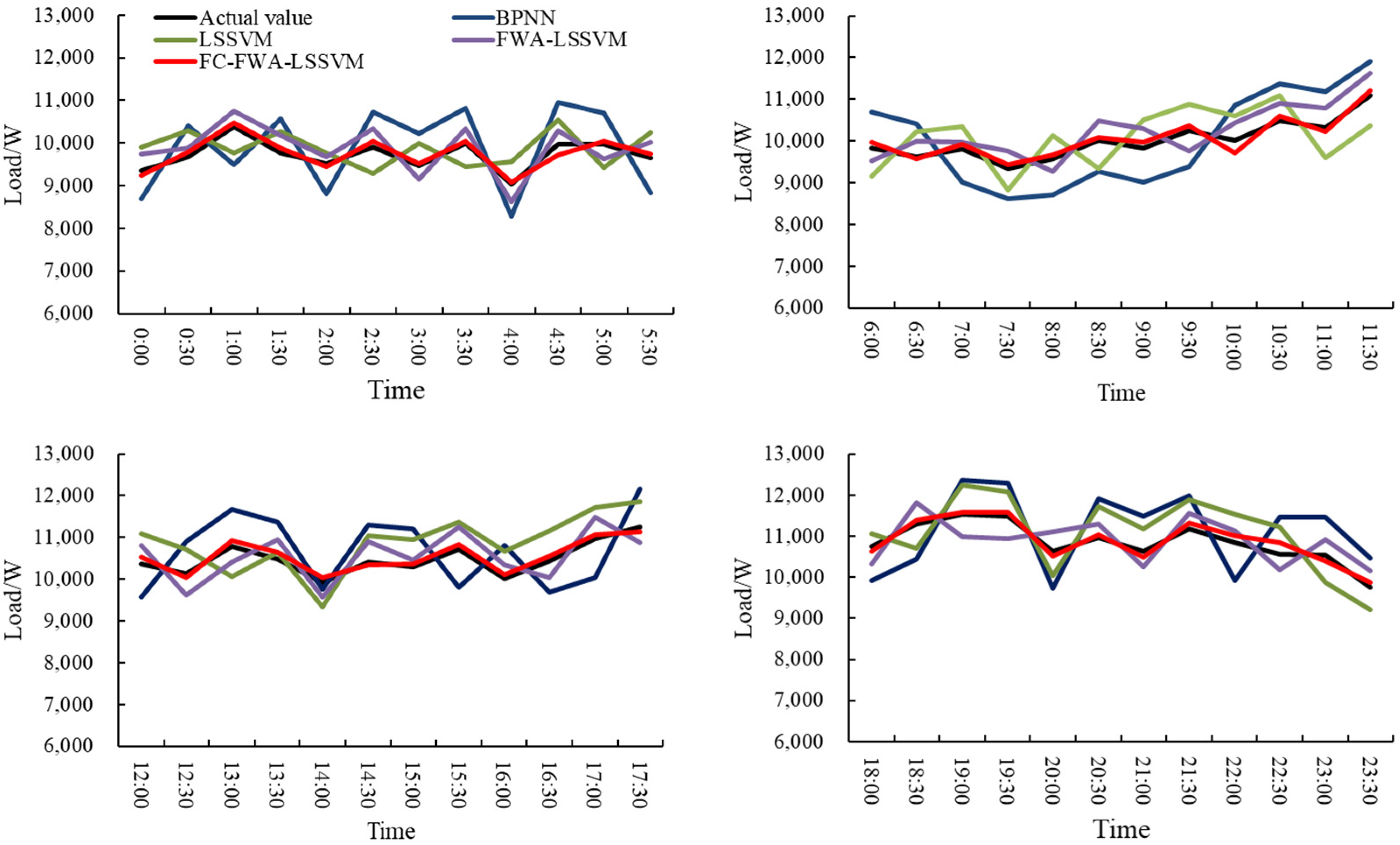
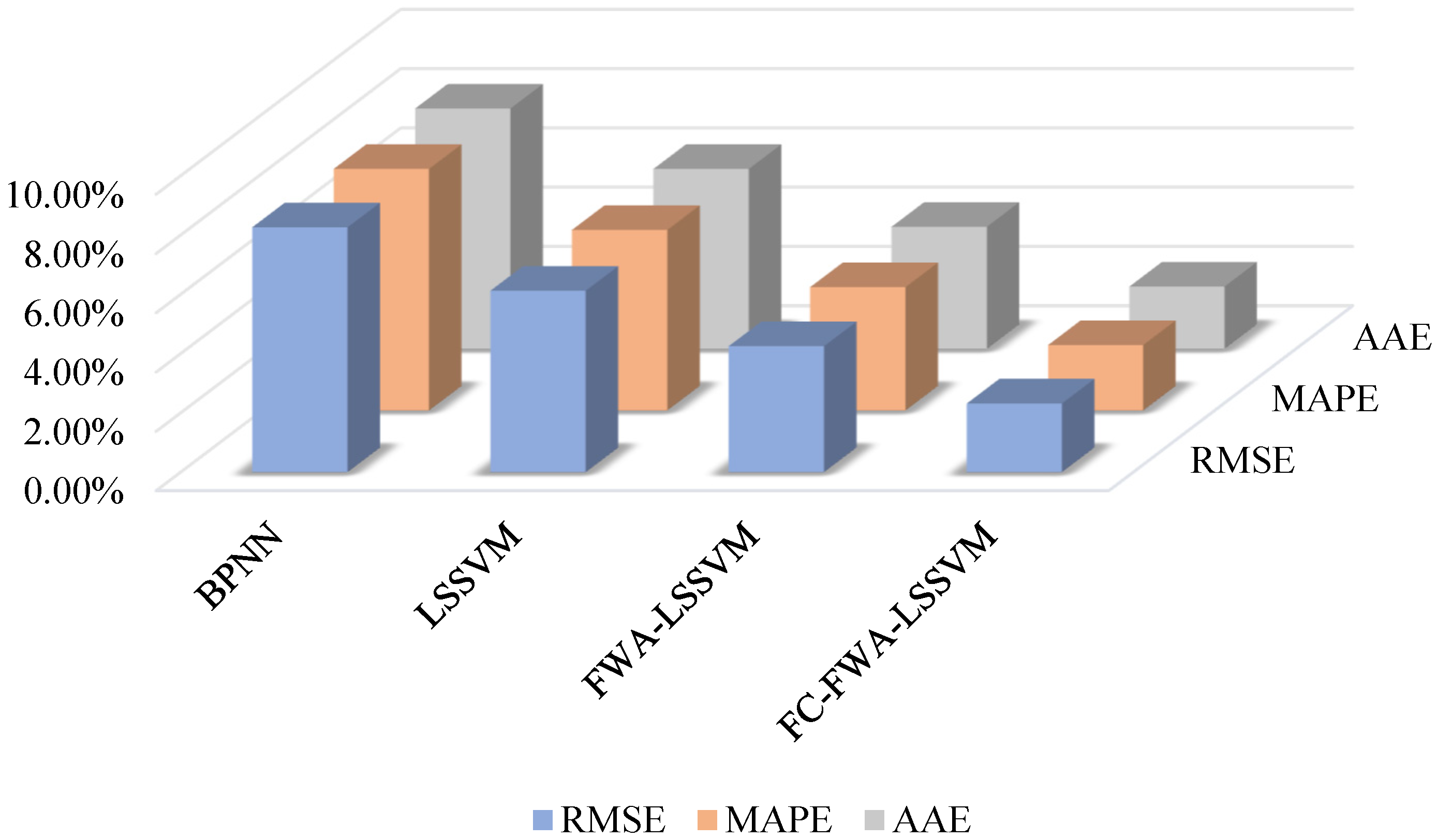
Initialize the FWA parameter: The highest size of cycles is $Maxgen=1000$, the size of the population is $PopNum=40$, the size of spark determines the constant $M=150$, and the radius of blast determines the constant $\widehat{x}=200$. To validate the performance of the prediction method presented in this article, this study relied on the test sample data and conducted comparison experiments using the fireworks-algorithm-optimized LSSVM model (FWA–LSSVM), the standard LSSVM model, and the standard BPNN model. Figure 2 and

Table 1. Prediction results.

Time	Actual Value	BPNN	LSSVM	FWA–LSSVM	FC–FWA–LSSVM
0:00	9357	8683	9904	9743	9239
0:30	9676	10,418	10,296	9870	9785
1:00	10,373	9487	9776	10,744	10,469
1:30	9763	10,570	10,273	10,168	9874
2:00	9510	8817	9765	9685	9452
2:30	9894	10,718	9289	10,326	10,030
3:00	9461	10,226	9991	9161	9527
…	…	…	…	…	…
19:00	11,524	12,369	12,235	10,976	11,582
19:30	11,483	12,299	12,074	10,942	11,586
20:00	10,644	9720	10,049	11,107	10,503
20:30	10,972	11,912	11,720	11,304	11,038
21:00	10,624	11,492	11,187	10,261	10,493
21:30	11,173	11,979	11,897	11,568	11,310
22:00	10,852	9930	11,537	11,126	11,006
22:30	10,559	11,455	11,214	10,173	10,856
23:00	10,531	11,473	9884	10,911	10,393
23:30	9746	10,470	9212	10,168	9879

show the forecasting results of the proposed model, FWA–LSSVM, LSSVM, and BPNN models for loads in this paper. Figure 3 and

Table 2. RE of each prediction model.

Time	BPNN (%)	LSSVM (%)	FWA–LSSVM (%)	FC–FWA–LSSVM (%)
0:00	−7.199	5.85	4.13	−1.265
0:30	7.667	6.41	2.01	1.133
1:00	−8.546	−5.757	3.575	0.924
1:30	8.27	5.232	4.156	1.136
2:00	−7.284	2.685	1.848	−0.61
2:30	8.321	−6.115	4.368	1.376
3:00	8.09	5.601	−3.165	0.7
…	…	…	…	…
19:00	7.335	6.168	−4.754	0.501
19:30	7.11	5.15	−4.713	0.899
20:00	−8.68	−5.591	4.348	−1.322
20:30	8.573	6.821	3.029	0.603
21:00	8.169	5.3	−3.42	−1.234
21:30	7.215	6.481	3.537	1.222
22:00	−8.496	6.306	2.526	1.418
22:30	8.484	6.206	−3.658	2.813
23:00	8.943	−6.149	3.6	−1.317
23:30	7.427	−5.475	4.325	1.367

show the RE of each prediction model.

From Figure 2 and Figure 3, we can infer that the prediction errors of the proposed model are controlled within (−3%, 3%) for all time points, with the smallest absolute value of 0.50% and the highest point of 2.99%; only three of them are outside the range of (−1.5%, 1.5%)—namely, −2.52% at 4:30, −2.99% at 10:00, and 2.81% at 22:30. The FWA–LSSVM prediction model has five time points with relative errors controlled in the range of (−3%, 3%)—namely, 2.01% at 0:30, 1.85% at 2:00, 1.45% at 7:00, 1.46% at 15:00, and 2.53% at 22:00, with the smallest absolute value of 1.45% and the highest point of 4.98%. The LSSVM model prediction results have the smallest absolute value of 1.62% and the highest point of 6.98%, and the majority of the time points are in the range of (−1.5%, 1.5%), with the smallest absolute value 1.62% and the highest point of −4%. The smallest absolute value of the relative error of the BPNN model is −1.55%, and the maximum value is 9.97%, and the errors of the majority of the time points are between (−7%, −5%) and (5%, 7%), with a large fluctuation. From this perspective, the FC–FWA–LSSVM model has the highest forecasting precision, followed by the FWA–LSSVM model and the LSSVM model, and the worst is the BPNN model. It can be seen that fuzzy clustering analysis can effectively prevent ignorance in choosing similar days by manual experience. Compared with the traditional LSSVM model, the FWA-optimized LSSVM model improved its prediction accuracy because it found better model arguments.

Figure 4 and

Table 3. RMSE, MAPE, and AAE of the prediction results.

	BPNN	LSSVM	FWA–LSSVM	FC–FWA–LSSVM
RMSE	8.26%	6.12%	4.25%	2.32%
MAPE	8.15%	6.09%	4.16%	2.21%
AAE	8.11%	6.07%	4.12%	2.10%

show the RMSE, MAPE, and AAE of each model for the overall prediction results. It is evident that the RMSE of the method presented in this article is calculated as 2.32%, while the RMSE of the FWA–LSSVM, LSSVM, and BPNN models are calculated as 4.25%, 6.12%, and 8.26%, respectively. This shows that the forecasting outcome of the model introduced in this article has small errors and the highest general precision of forecasting. Additionally, the FC–FWA–LSSVM model has the best-calculated results for MAPE (2.21%) and AAE (2.10%). Compared with the FWA–LSSVM model, fuzzy clustering analysis overcomes, to some extent, the negative impact of non-conventional load data on LSSVM training due to unexpected changes in influencing agents. Contrasting this with the LSSVM model reveals that its generalization capability and forecasting precision can be enhanced by enhancing the arguments of the LSSVM. In contrast to the BPNN model, the LSSVM model can protect against the disadvantages of delayed restraint and the tendency to become stuck in a local optimum of the BPNN model. Overall, the FC–FWA–LSSVM model has the best forecasting performance, the FWA–LSSVM model and the LSSVM model are the next best, and the BPNN model has the worst prediction performance.

5. Scenario Validation

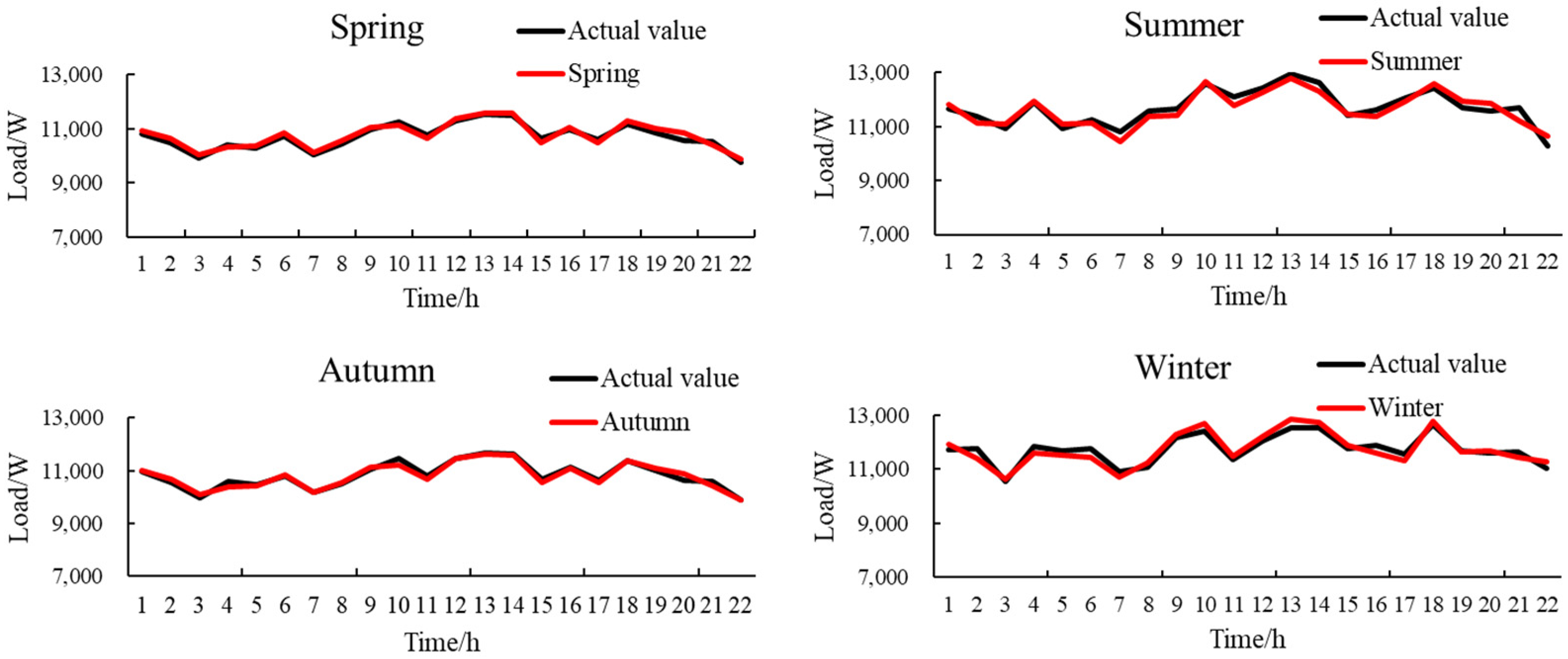
To remove the specificity of the target day and to check the generalization behavior of the model, one day of data from each of the four seasons was picked as the test sample: 17 April as the spring test sample; 21 July as the summer test day; 9 October as the autumn test day; 28 January as the winter test day.

Figure 5 shows the curve of the forecasting load values against the true values of the load for the four seasons of spring, summer, autumn, and winter.

By comparing the predicted and true load values for the four seasons, it can be concluded that the total predicted tendency of all four models is near to the true value, which validates the advantages of the model proposed in this paper for residential electricity load forecasting.

From

Table 4. RMSE, MAPE, and AAE of the prediction results.

Season	Index	FC–FWA–LSSVM
Spring	RMSE	2.09%
	MAPE	2.21%
	MAE	2.03%
Summer	RMSE	2.01%
	MAPE	2.08%
	MAE	2.44%
Autumn	RMSE	2.21%
	MAPE	2.17%
	MAE	2.03%
Winter	RMSE	2.19%
	MAPE	2.32%
	MAE	2.40%

, it can be concluded that the RMSE, MAPE, and MAE values of the FC–FWA–LSSVM forecasting model proposed in this paper are the lowest for the four seasonal test samples, as shown in the table. The RMSE, MAPE, and MAE values for spring load forecasting are 1.3901%, 1.4112%, and 1.4349%, respectively; the RMSE, MAPE, and MAE values for summer load forecasting are 1.3912%, 1.5812%, and 1.4424%; the RMSE, MAPE, and MAE values for summer load forecasting are 1.5123%, 1.4671%, and 1.4291%; the RMSE, MAPE, and MAE values for winter load forecasting are 1.3941%, 1.4214%, and 1.4042%, all of which are lower than the other models; this, again, illustrates the optimal overall prediction performance of the prediction model proposed in this paper.

6. Conclusions

In this article, we presented a hybrid load forecasting model that combines fuzzy cluster analysis and LSSVM and is optimized by FWA. First, to forecast residential electric load loads, fuzzy cluster analysis was used to select the input features. In addition, FWA was used to optimize the criteria of LSSVM. Finally, upon acquiring an optimized feed subset and the optimal values of γ and σ², the proposed model was used for residential electricity load forecasting. Based on these studies, several conclusions can be drawn as follows: (a) By using fuzzy clustering analysis, the influence of uncorrelated factors can be mitigated, which effectively improves forecasting capabilities; (b) the optimization algorithm FWA increases the global search capability of the model, and the LSSVM model optimized by FWA shows good performance; (c) based on the error evaluation criteria, with SVM, LSSVM achieves better prediction results, indicating that the method of improving SVM by introducing least-squares linear system is effective. The model based on FCA and KELM optimized with FWA proposed in this paper offers a new research direction for load forecasting and is highly feasible. In the example of load forecasting, the desired forecasting results were obtained. In future research, the forecasting model can be applied to develop demand corresponding strategies to contribute to peak and valley reduction in electricity loads.

References

1. Fan, Y.N.; Chen, C.H.; Xu, J.Y.; Xu, L.; Yu, D. Medium- and long term power load forecasting based on MATLAB gray Elman network. Tech. Autom. Appl. 2021, 40, 93–98. [Google Scholar]
2. Chen, J.P.; Hu, Z.J.; Chen, W.N.; Gao, M.; Du, Y.; Lin, M. Load prediction of integrated energy system based on combination of quadratic modal decomposition and deep bidirectional long short-term memory and multiple linear regression. Autom. Electr. Power Syst. 2021, 45, 85–94. [Google Scholar]
3. Zhang, H.; Li, S.X.; Shi, J.; Liu, X.; Wang, K.; Sun, X. Short-term load forecasting method based on serial GA-BP. Proc. CSU-EPSA 2021, 33, 97–101. [Google Scholar]
4. Li, Z.W.; Hu, J.A.; Liu, X.; Deng, Y.; Tang, P.; Wang, Y. Multi-factor short-term load prediction model based on PCA-DBILSTM. Proc. CSU-EPSA 2020, 32, 32–39. [Google Scholar]
5. Bozorg, M.; Bracale, A.; Caramia, P.; Carpinelli, G.; Carpita, M.; De Falco, P. Bayesian bootstrap quantile regression for probabilistic photovoltaic power forecasting. Prot. Control Mod. Power Syst. 2020, 5, 218–229. [Google Scholar] [CrossRef]
6. Xi, Y.W.; Wu, J.Y.; Shi, C.; Zhu, X.; Cai, R. A refined load forecasting based on historical data and real-time influencing factors. Power Syst. Prot. Control 2019, 47, 80–87. [Google Scholar]
7. Chen, H.; Zhang, J.; Tao, Y.; Tan, F. Asymmetric GARCH type models for asymmetric volatility characteristics analysis and wind power forecasting. Prot. Control Mod. Power Syst. 2019, 4, 29. [Google Scholar] [CrossRef] [Green Version]
8. Cheng, C. Improved BP Neural Network Based on Genetic Algorithm for Short-Term Load Forecasting of Power System. Master’s Thesis, Xi’an University of Technology, Xi’an, China, 2020. [Google Scholar]
9. Zhao, P.; Dai, Y.M. Power load forecasting of SVM based on real-time price and weighted grey relational projection algorithm. Power Syst. Technol. 2020, 44, 1325–1332. [Google Scholar]
10. Lin, Z.R.; Li, J.C.; Yang, D.Q.; Jun-Yun, W.U. Network traffic prediction based on wavelet neural network with improved differential evolution algorithm. Comput. Eng. Design. 2019, 40, 3413–3418. [Google Scholar]
11. Liang, Y.; Wang, H.C.; Hong, W.C. Sustainable Development Evaluation of Innovation and Entrepreneurship Education of Clean Energy Major in Colleges and Universities Based on SPA-VFS and GRNN Optimized by Chaos Bat Algorithm. Sustainability 2021, 13, 5960. [Google Scholar] [CrossRef]
12. Yan, C.; Tang, Y.; Dai, J.; Wang, C.; Wu, S. Uncertainty modeling of wind power frequency regulation potential considering distributed characteristics of forecast errors. Prot. Control Mod. Power Syst. 2021, V6, 276–288. [Google Scholar] [CrossRef]
13. Wang, Y.L.; Zhou, M.H.; Yao, S.H.; Wei, M.J.; Yang, Y.; Liu, Z.; Hu, M.J. Multi-load cooperative prediction model of integrated energy system based on multi-energy coupling mechanism. J. North China Electr. Power Univ. (Nat. Sci. Ed.) 2021, 1–10. Available online: https://kns.cnki.net/kcms/detail/13.1212.tm.20210705.1544.002.html (accessed on 15 December 2021).
14. Hu, L.J.; Guo, C.Z.; Wang, J.S. Short-term Power Load Forecasting Based on ISSA-LSSVM Model. Sci. Technol. Eng. 2021, 21, 9916–9922. [Google Scholar]
15. Wang, H.; Liang, Y.; Ding, W.; Niu, D.; Li, S.; Wang, F. The Improved Least Square Support Vector Machine Based on Wolf Pack Algorithm and Data Inconsistency Rate for Cost Prediction of Substation Projects. Math. Probl. Eng. 2020, 2020, 6663006. [Google Scholar] [CrossRef]
16. Liu, X.D.; Zou, Y.N.; Xiong, X.D.; Cheng, C.; Yang, H.Y. A regional load forecasting method based on improved Cuckoo Search LSSVM. Inf. Technol. 2021, 45, 41–47. [Google Scholar]
17. Han, P.P.; Pan, W.; Zhang, N.; Wu, H.; Qiu, R.; Zhang, Z. Optimization method for artificial phase sequence based on load forecasting and non-dominated sorting genetic algorithm. Autom. Electr. Power Syst. 2020, 44, 71–78. [Google Scholar]
18. Guan, S.H.; Shen, Y.X. Power load forecasting based on PSO RBF-NN. Transducer Microsyst. Technol. 2021, 40, 128–131. [Google Scholar]
19. Erdiwansyah, M.; Husin, H.; Nasaruddin, M.Z.; Muhibbuddin, A. Critical review of the integration of renewable energy sources with various technologies. Prot. Control Mod. Power Syst. 2021, 6, 37–54. [Google Scholar] [CrossRef]
20. Wu, Y.; Lei, J.W.; Bao, L.S.; Li, C.Z. Short-term load forecasting based on improved grey correlation analysis and neural network optimized by bat algorithm. Autom. Electr. Power Syst. 2018, 42, 67–72. [Google Scholar]
21. Wang, Y.F.; Zheng, Y.P.; Xue, H. Optimal dispatch of mobile energy storage for peak load shifting based on enhanced firework algorithm. Autom. Electr. Power Syst. 2021, 45, 48–56. [Google Scholar]
22. Soh, W.; Kim, H.; Yum, B.-J. Application of kernel principal component analysis to multi-characteristic parameter design problems. Ann. Oper. Res. 2018, 263, 69–91. [Google Scholar] [CrossRef]
23. Xie, L.; Li, Z.; Zeng, J.; Kruger, U. Block adaptive kernel principal component analysis for nonlinear process monitoring. AIChE J. 2016, 62, 4334–4345. [Google Scholar] [CrossRef]
24. Wang, R.; Chen, S.W.; Lu, J. Time-division refined short term load forecasting based on BOA-SVR and Fuzzy Clustering. Eng. J. Wuhan Univ. 2021, 1–10. [Google Scholar]
25. Filho, J.B.O.S.; Diniz, P.S.R. A Fixed-Point Online Kernel Principal Component Extraction Algorithm. IEEE Trans. Signal Process. 2017, 65, 6244–6259. [Google Scholar] [CrossRef]
26. Omar Noureldeen, I. Hamdan. A novel controllable crowbar based on fault type protection technique for DFIG wind energy conversion system using adaptive neuro-fuzzy inference system. Prot. Control Mod. Power Syst. 2018, 3, 328–339. [Google Scholar]
27. Dong, W.C.; Li, S.H. Reliability sensitivity of wind power system considering correlation of forecast errors based on multivariate NSTPNT method. Prot. Control Mod. Power Syst. 2021, 6, 136–146. [Google Scholar] [CrossRef]
28. Shang, L.; Zhu, W.; Li, P.; Guo, H. Maximum power point tracking of PV system under partial shading conditions through flower pollination algorithm. Prot. Control Mod. Power Syst. 2018, 3, 400–406. [Google Scholar] [CrossRef]
29. Zheng, D.; Eseye, A.; Zhang, J.; Li, H. Short-term wind power forecasting using a double-stage hierarchical ANFIS approach for energy management in microgrids. Prot. Control Mod. Power Syst. 2017, 2, 136–145. [Google Scholar] [CrossRef] [Green Version]
Figure 1. The proposed composite prediction framework.
Sustainability 14 01312 g001
Figure 2. Prediction results.
Sustainability 14 01312 g002
Figure 3. RE of each prediction model.
Sustainability 14 01312 g003
Figure 4. RMSE, MAPE, and AAE of the prediction results.
Sustainability 14 01312 g004
Figure 5. Electricity load forecast graph.
Sustainability 14 01312 g005