Fault Detection of Wind Turbine Blades Using Multi-Channel CNN

Abstract

This study utilized the multi-channel convolutional neural network (MCNN) and applied it to wind turbine blade and blade angle fault detection. The proposed approach automatically and effectively captures fault characteristics from the imported original vibration signals and identifies their state in multiple convolutional neural network (CNN) models. The result obtained from each model is sent to the output layer, which is a maximum output network (MAXNET), to compute the most accurate state. First, in terms of wind turbine blade state detection, this paper builds blade models based on the normal state and three common fault types, including blade angle anomaly, blade surface damage, and blade breakage. Vibration signals are employed for fault detection. The proposed wind turbine fault diagnosis approach adopts a triaxial vibration transducer and frame grabber to capture vibration signals and then applies the new MCNN algorithm to identify the state. The test results show that the proposed approach could deliver up to 87.8% identification accuracy for four fault types of large wind turbine blades.

1. Introduction

As wind turbines are exposed outdoors for long periods, there is a high probability that their parts will become aged and worn after long-term operations. According to historical data, a number of wind turbine damage incidents have been recorded so far [1,2,3,4,5,6,7,8,9,10,11,12,13]. Common wind turbine faults include engine room overtemperature, gearbox damage, blade breakage, and bearing damage. However, wind turbines must often be removed from service for a long time when key components become faulty, thereby reducing their green power generation efficiency. A literature review found that most prior studies on wind turbine troubleshooting focus on wind turbine gearboxes [1,2], bearings [3,4,5,6,7], generators [8,9], and blades [10,11,12,13,14,15]. Malik et al. [12] proposed a wind turbine state monitoring approach based on an artificial neural network (ANN) and empirical mode decomposition (EMD) and modeled a wind turbine by applying MATLAB/Simulink. This approach was applied to analyze whether wind turbines were balanced and stable by analyzing the blades, engine rooms, tails, rotors, and other aerodynamic parts. Further, Yang et al. [13] proposed a blade vibration dynamics and frequency analysis approach based on frequency indexes, which was applied to low-speed wind turbine blades made of 29-inch glass fibers. When cracks are present on a blade, this approach can clearly identify their positions. Sahoo et al. [14] proposed the use of machine-learning algorithms, such as k-nearest neighbor (KNN), support vector machine (SVM), and decision tree, together with accelerometers for capturing vibration signals at different speeds and for the fault detection of wind turbine blades. The fault types were a healthy blade, a bent blade, a cracked blade, and an eroded blade. According to the results, the identification accuracy of SVM was the highest (87%), followed by the decision tree (82%) and KNN (80.8%). Liu et al. [15] proposed a method combining the deep belief network (DBN) with batch normalization for the vibration signal fault detection of wind turbine gearboxes and stated its advantage of avoiding overfitting of the training model. The fault types were normal, wear, and tooth broken. According to the results, the identification accuracy of this method (Normal: 100%; Wear: 99%; Tooth broken: 98%) was higher than that of the BPNN, SVM, and Softmax functions. Yu et al. [16] proposed a new fast deep graph convolutional network (FDGCN) to carry out the wavelet packet transform (WPT) on the original vibration signals of wind turbine gearboxes and then transformed the signals from the time domain features into graphs, which were input into the FDGCN for the gearbox vibration signal analysis. The fault types were normal, chipped tooth gear, eccentric gear, missed tooth gear, ball fault on a bearing, inner raceway fault on a bearing, outer raceway fault on a bearing, and composite fault on a bearing. According to the results, the accuracy rate of this method was 93.09%, which was higher than WDCNet (87.66%), LeNet (88.33%), ResNet (90.43%), and GCNet (90.25%). Firuzi et al. [17] transformed phase-resolved partial discharge (PRPD) images into grayscale images to express different partial discharge types, which were followed by feature extraction employing the traditional histogram of oriented gradients (HOG) method and the local binary pattern (LBP) method. Finally, the SVM classifier was utilized to identify partial discharge types. While most studies focus on cracks on the blade surface, few have proposed a wind turbine simulation and detection platform built based on the IoT and AI for blade pitch anomalies (mechanical failure) and blade breakage. Hu et al. [18] proposed a multichannel 2D convolutional neural network (CNN) model that included three parts of the 2D CNN architecture in parallel with a fully connected hidden layer to classify 3D task-based functional magnetic resonance imaging (fMRI) data. The method transforms 3D fMRI images into multichannel 2D (M2D) images for learning with an M2D CNN network and integrates multichannel information from three 2D CNNs. Schwenk et al. [19] proposed an adaptive boosting method to enhance the performances of neural networks for auto-associative (Diabolo) networks and multi-layer neural networks (MLPs) on character recognition tasks. The results showed that the weighted training of the adaptive boosting operates well for MLP but needs more training epochs. Saghafinia et al. [20] presented an online trained fuzzy logic controller (FLC) and adaptive continuous wavelet transform (CWT) high precision fault detection for a three-phase squirrel cage induction motor (IM) with broken rotor bars. The results found that the method can accurately detect IM faults based on the motor’s current signal at different fault and load conditions. Juan et al. [21] proposed a novel data-driven diagnosis methodology based on autoencoder deep feature learning (unsupervised neural network) used to diagnose and identify bearing faults, including metallic, ceramic bearings, and hybrid in electromechanical systems. The approach can overcome the challenge of noise immunity and consider it as a part of the condition-monitoring strategies. Jiang et al. [22] introduced a new feature representation learning approach called the stacked multilevel-denoising autoencoders to learn robustly and distinguish fault feature expressions for feature extraction and classification of wind turbine gearbox fault diagnosis. The results showed that the method could improve the conventional stacked denoising autoencoder and achieve good diagnosis accuracies.

Therefore, this study constructed blade models for wind turbine blade state detection based on the normal state and three common fault types, including blade angle anomaly, blade surface damage, and blade breakage. This study built an intelligent detection system for wind turbines based on a multi-channel convolutional neural network (MCNN) and designed wind turbine blade models based on four states of fiber-reinforced plastic (FRP) blades. Data were captured using an NI PXI high-speed data acquisition (DAQ) instrument. Wind turbine troubleshooting was performed based on data processing and MCNN. The proposed wind turbine blade fault characteristic learning model was expected to identify blade fault types accurately so that early maintenance and preventive measures could be taken to prevent accidents. The proposed MCNN model is an improvement on traditional CNN due to the integration of multiple CNN models. It implements fault diagnoses based on different input data and can identify the state type in multiple CNN models while directly and automatically generating characteristic diagrams from the original vibration signals. The proposed MCNN can deal with different cases of wind turbine models with an unknown nonlinear input and under unknown wind velocity conditions. It has a multi-channel learning capability that provides two advantages over traditional CNN: (1) the layered learning structure based on multiple convolutional and pooling layers can effectively identify fault characteristics; and (2) multi-channel learning provides a better identification capability for different data. Therefore, the proposed approach could improve the fault identification rate.

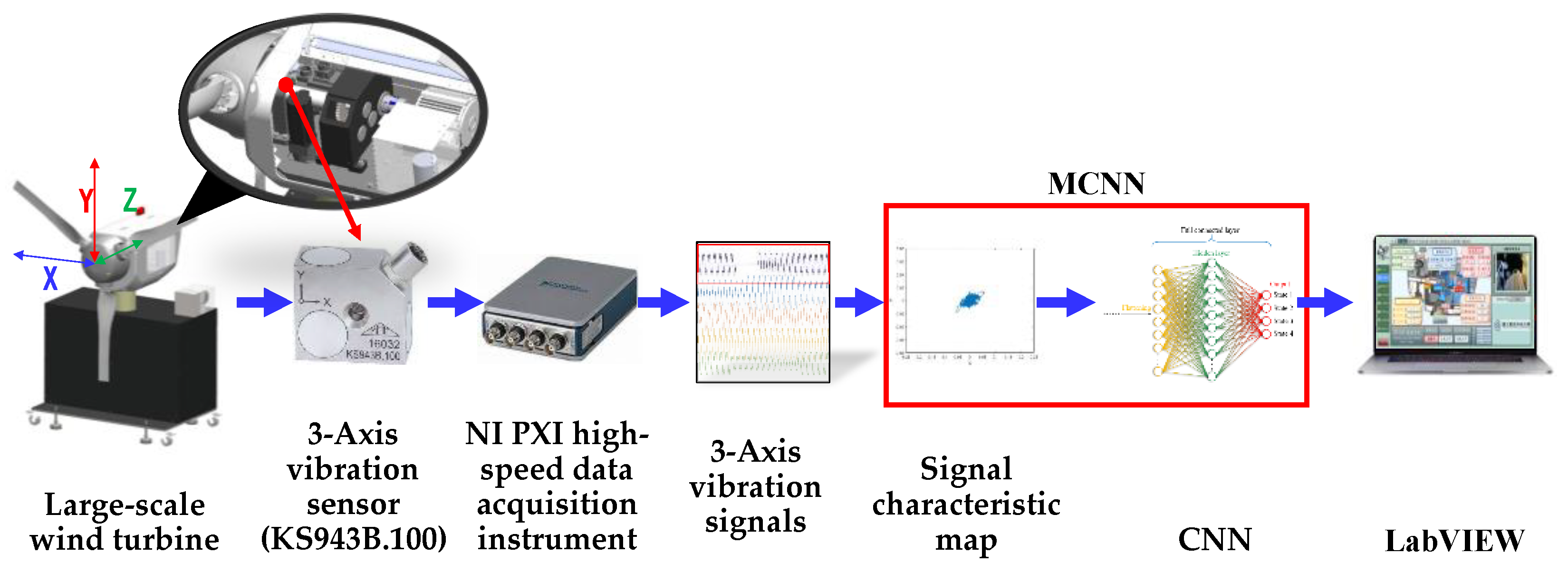
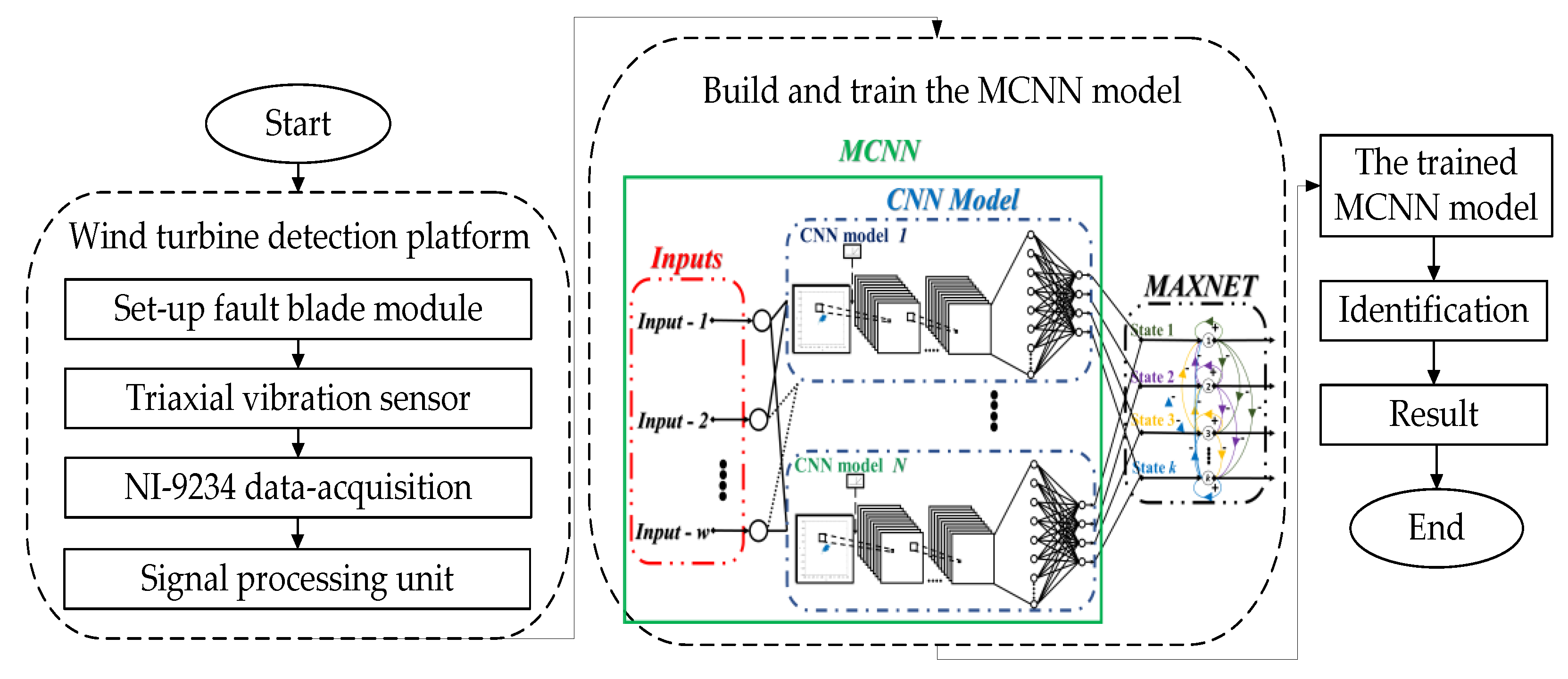
2. System Architecture

The proposed approach aimed to detect the fault types of wind turbine blades and blade angles. Figure 1 shows the architecture of the proposed system. The wind turbine is mainly driven by a servo motor to control the situation of wind rotating the blades (the wind turbine operating speed is 12 rpm), and a triaxial vibration sensor (KS943B.100) was installed on the rotor bearing near the blades to measure their vibration signals. Wind turbine blade fault types were built based on the normal state, blade angle anomaly, blade surface damage, and blade breakage. Front-end vibration signals were captured and then imported through the signal processing unit to the MCNN to generate signal characteristic diagrams and identify the fault types. The following section explains the capture of the wind turbine vibration signals and the fault modeling.

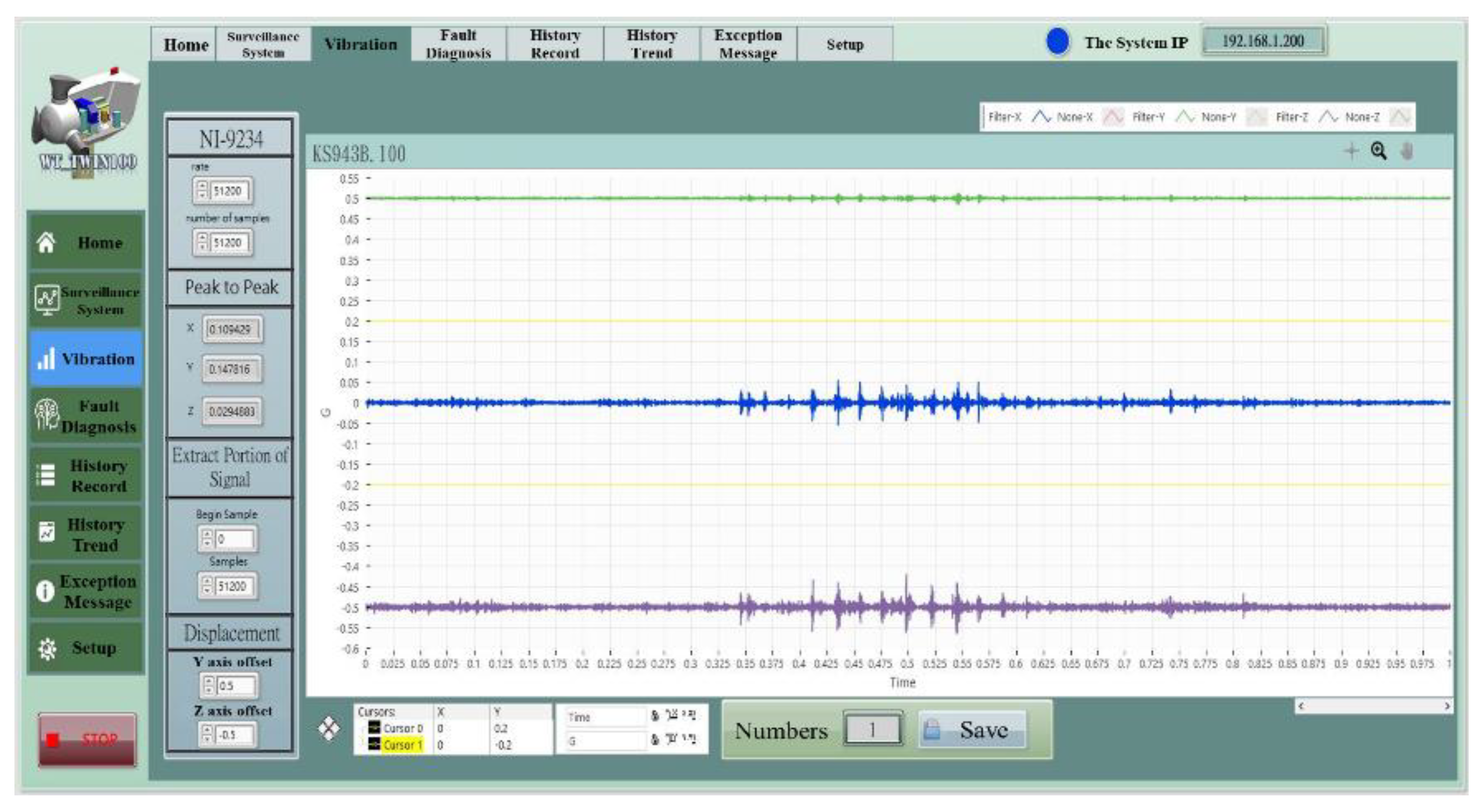
2.1. Capture of Wind Turbine Blade Fault Signals

To detect abnormal vibration phenomena caused by wind turbine blade faults, this paper developed a human–machine interface system for wind turbine vibration analysis and detection in LabVIEW, as shown in Figure 2. Signals were first converted into voltage signals through a triaxial vibration transducer. The vibration signals were then sent to the human–machine interface by the NI PXI high-speed data acquisition instrument, and lastly, the MCNN identified the blade and blade angle.

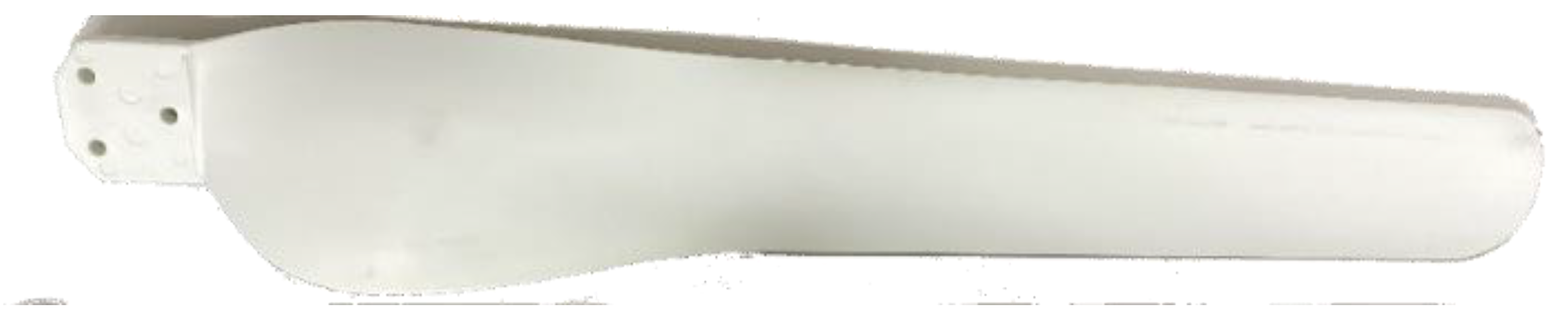
2.2. Wind Turbine Blade Fault Modeling

Dao et al. [23] pointed out that after running in a harsh environment for an extended period, wind turbine blades may be subject to surface damage and breakage, and the blade angle system may become abnormal due to mechanical fatigue. To this end, this paper built wind turbine blade models (State 1) based on the normal state and three common blade faulty state models (State 2 to State 4) to discuss the vibration signals generated when wind turbine blades are in different states. Further, a signal processing and conversion system was used to filter the vibration signals. The blades in this paper were customized by the wind turbine manufacturer according to actual commercial wind turbines. The blades were made of fiber-reinforced polymer (FRP), had a length of 70 cm, and were solid inside. Lastly, MCNN was used to identify the state. The built wind turbine blade models are described in the following subsections.

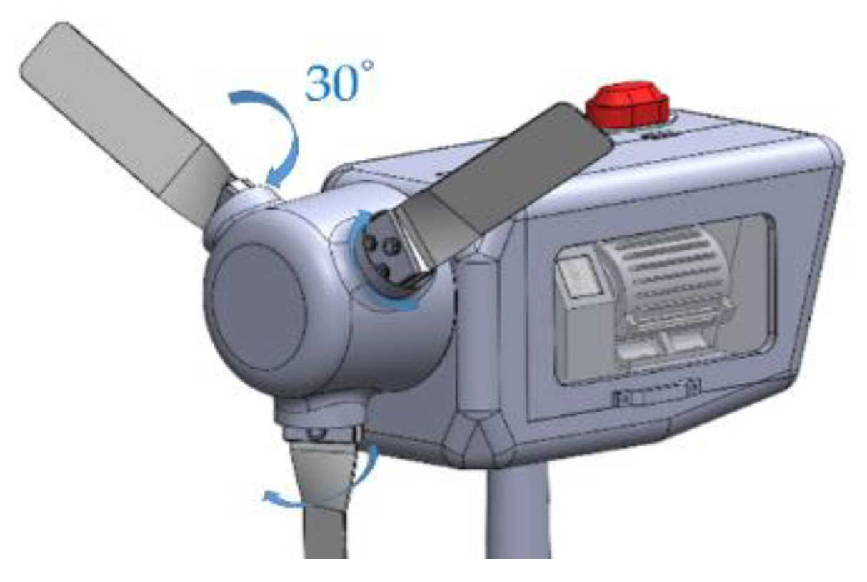
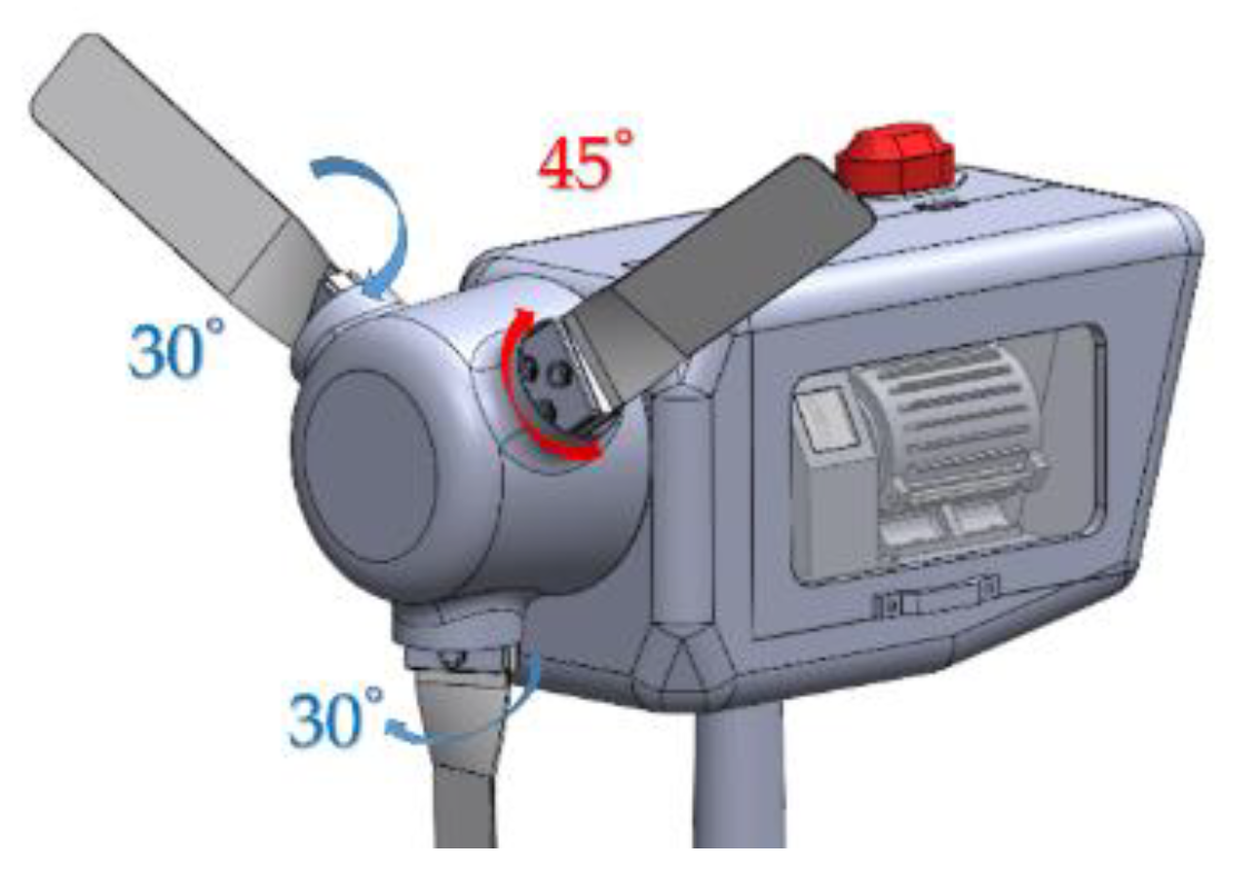
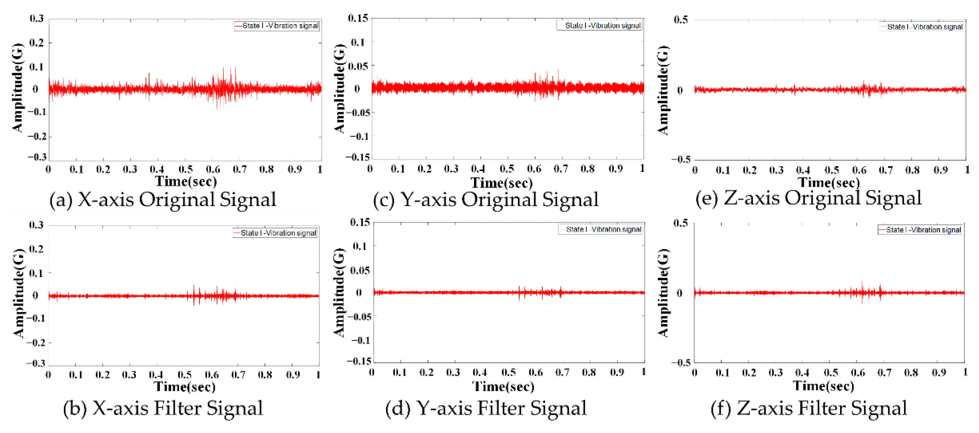
2.2.1. Normal Wind Turbine Blades (State 1)

Currently, most wind turbine manufacturers adopt composite materials to manufacture wind turbine blades and use FRP to manufacture the shells. Therefore, this paper employed wind turbine blades made of FRP, as shown in Figure 3. These blades were 70 cm long and had an efficient rotating blade shape. Figure 4 shows blades installed on a wind turbine and run at a blade angle of 30°.

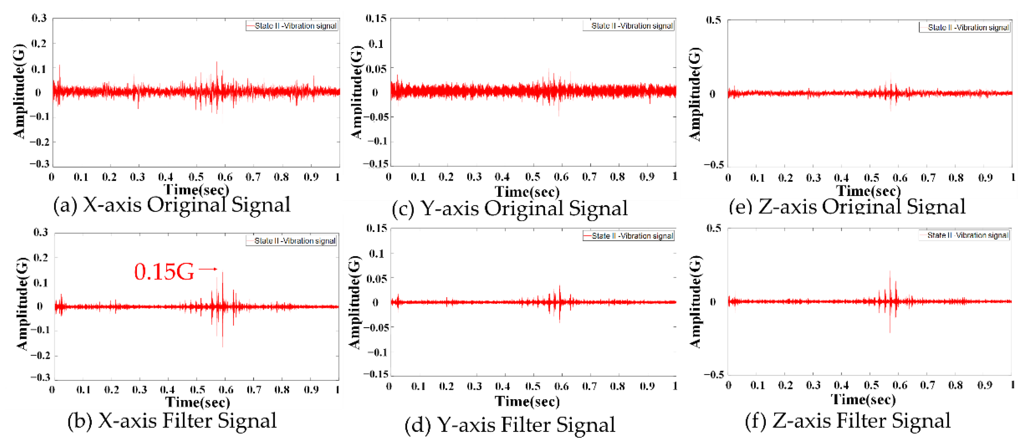
2.2.2. Blade Angle Anomaly (State 2)

Wind turbines must often cope with high wind loads and asymmetric wind directions. After a wind turbine runs for a long period, the blade angle system will become worn, and parts may be damaged [24,25]. That is, if a wind turbine runs outdoors for a long period, the blade angle will become abnormal, or the angle will become unbalanced due to mechanical fatigue. Therefore, defects caused by angle system faults were constructed and analyzed in this paper. Current blade angle systems are designed using speed-varying rotor and collective pitch control (CPC) technologies. However, these technologies contribute to limited improvement. If the blade angles of three blades on a wind turbine run differently for a long period, the wind turbine system will become imbalanced. As a result, the system may be damaged, and the wind turbine could even collapse. Therefore, in this paper, one blade angle of the three blades was adjusted to 45° to simulate the blade angle control and generate and record vibration signals when one blade angle failed to be synchronized, as shown in Figure 5.

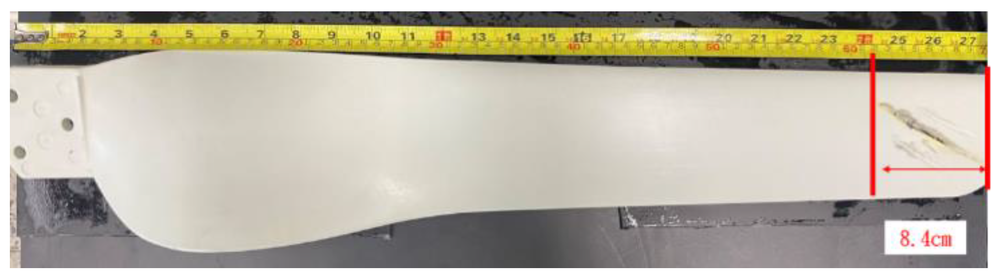
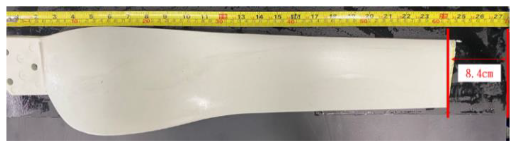
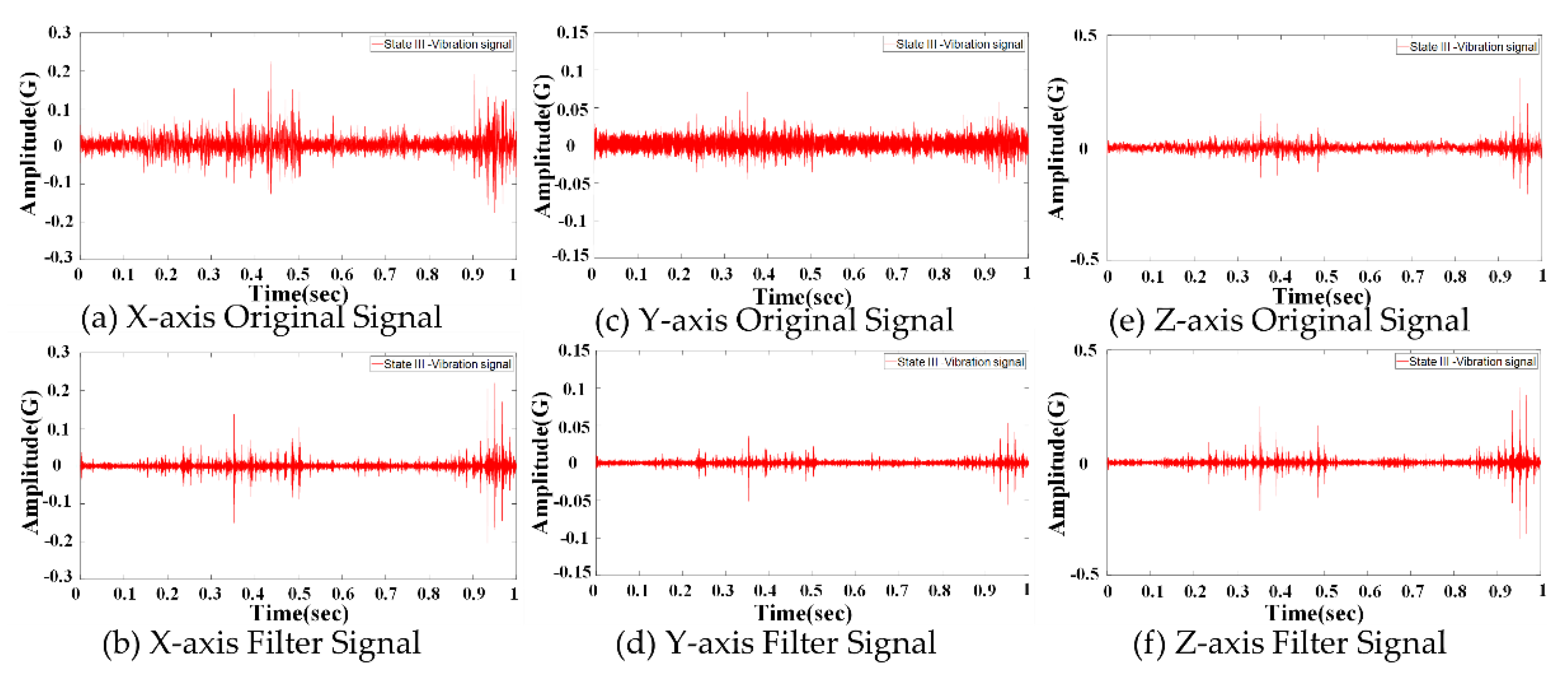
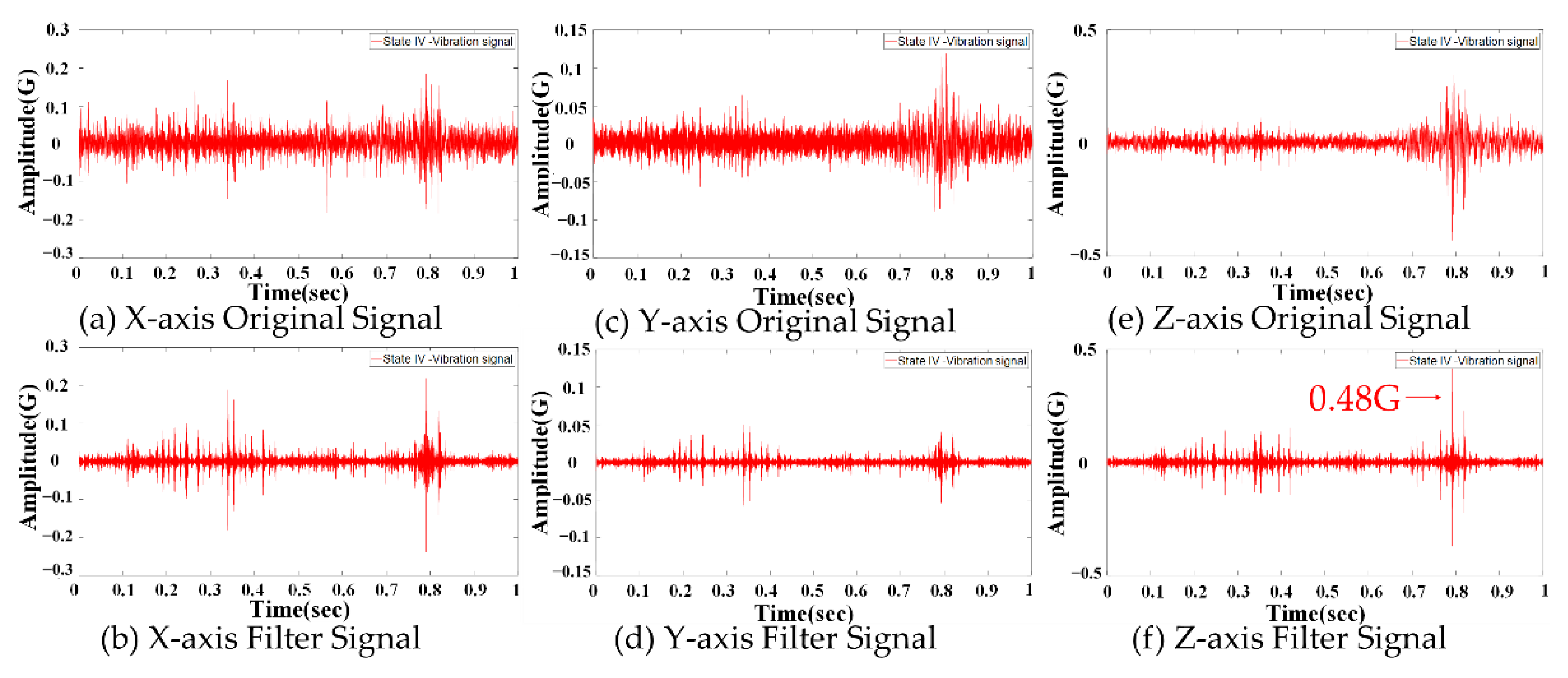
2.2.3. A Blade Suffering a Lightning Strike (State 3 and State 4)

As wind turbines are often erected in open areas, there is a high probability that they will suffer lightning strikes. According to [26,27,28] and IEC 61400-24 [29], the part of a wind turbine most likely to suffer a lightning strike is its blades. A lightning strike will severely damage the blade structure and surface materials, resulting in high repair costs. According to the statistics in [30], the front and rear parts of a blade are most likely to be damaged. Meanwhile, based on an analysis of the number of blades damaged by a lightning strike, one blade is highly likely to be damaged. Therefore, this paper analyzed models (State 3 and State 4) simulating the surface damage and breakage of one blade.

According to the investigation of a large-scale wind turbine blade failure report [26], it is pointed out that blade surface cracks and breakages often occur on the front part of a blade. Therefore, this study employed 70-cm blades for modeling and made surface damages at an 8.4 cm position. Figure 6 shows the model of the surface damage, and Figure 7 shows the broken blade.

3. Proposed Fault Diagnosis Algorithm

During blade state detection, the vibration signals measured by vibration sensors will inevitably be interfered with by the surrounding environment or affected by the detection instruments. All of these will add difficulty to the detection of faults. Therefore, a front-end signal processing unit was adopted to filter noise interference and improve signal analysis and identification. The proposed MCNN was used to import the triaxial vibration signals of the normal state and three faulty states into the system to generate three sets of signal characteristic diagrams for different blade states, and then MCNN identified the states. Figure 8 shows the wind turbine fault diagnosis process. The following explains CNN and MCNN.

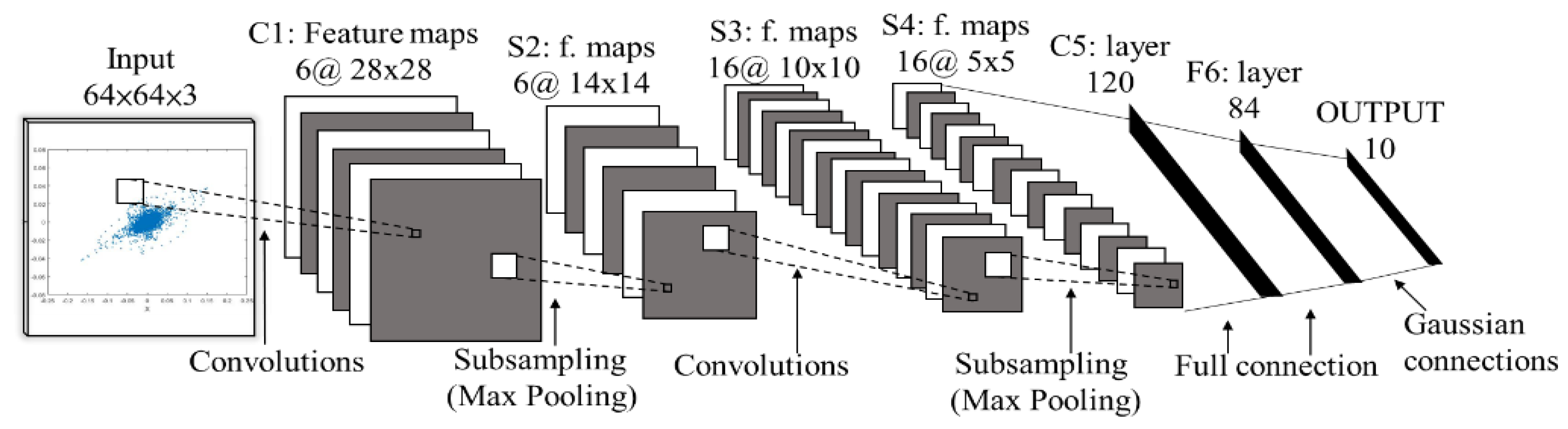
3.1. Convolutional Neural Network

In recent years, CNN has been widely applied to signal processing and image analysis in areas such as face recognition [31], medical imaging [32], and troubleshooting [33], and it has shown good performance. Classical CNN models include LeNet, AlexNet, VGG, GoogLeNet, and ResNet. In particular, LeNet [34] is considered the ancestor of the CNN models, as all CNN models have evolved from the LeNet architecture. Figure 9 shows the architecture of LeNet. The main architecture of a CNN model mainly comprises multiple convolutional layers, pooling layers, fully connected layers, and activating layers. The following introduces the layers in detail.

3.1.1. Convolution Layer

Convolutional layers in the CNN architecture are mainly responsible for capturing characteristics. They execute convolution computations through convolution kernels (also called filters) of different sizes and apply spatial filtering to extract or enhance the characteristics of images. The convolution kernel size has a direct effect on the characteristic detection performance. If the size of a convolution kernel is insufficient, the image identification performance may be poor. Meanwhile, if the size of a convolution kernel is excessively large, the time cost of computation will be increased. Generally, a 3 × 3 convolution kernel is employed for convolution computations of 7 × 7 images.

3.1.2. Pooling Layer

After an image passes through the convolutional layers and its characteristics have been obtained, the characteristics are added to the pooling layers to effectively reduce the size of the characteristic parameters and maintain their homogeneity. This can also simplify the computation over the network and make the pooled information focus on whether consistent characteristics exist in the image. Commonly-used pooling methods include max pooling and average pooling.

3.1.3. Fully Connected Layer

The architecture of the fully connected layers represents an artificial neural network comprised of flat, hidden, and output layers. These layers work to obtain the convolution computation and pooling results and adjust the errors between inputs and outputs through backpropagation. Finally, they employ the results to classify the images.

3.1.4. Activation Layer

The activation layers work to enhance the nonlinearity of the network. Commonly adopted activation functions are Sigmoid, Hyperbolic Tangent (tanh), Rectified Linear Unit (ReLu), and the recently-proposed Swish. Sigmoid was widely applied in the early days. However, the saturation phenomenon occurs when its variables are too small or too large, which likely results in the absence of gradient during backpropagation; hence, the network parameters cannot be effectively trained. In addition, complex computations will extend the network training duration.

3.2. Multi-Channel Convolutional Neural Network

Multi-channel convolutional neural network (MCNN) is an algorithm proposed in this paper and can be applied to fault diagnoses with multiple inputs. Unlike traditional approaches, it can identify the state type in multiple CNN models while directly and automatically generating characteristic diagrams from the original vibration signals. The MCNN then sends the identification result for each model to the back-end MAXNET for computation. Multiple signal sets can be input and generate a characteristic diagram to produce multiple CNN models at the input layer, to be classified by MAXNET. The design and parameters selection of MCNN, including layers, convolutional kernel size, activation, and pooling, are in

Table 1. The design and parameters selection of MCNN.

Channel	Layers of CNN	Convolutional Kernel Size	Activation	Pooling
1st CNN channel XY axis	11	3 × 3	ReLu	Max pooling
2nd CNN channel YZ axis	11	7 × 7	ReLu	Max pooling
3rd CNN channel XZ axis	11	7 × 7	ReLu	Max pooling

.

The state type selected by most frameworks is determined as the final identification result. The following subsection explains the architecture of MCNN and the generation of signal characteristic diagrams.

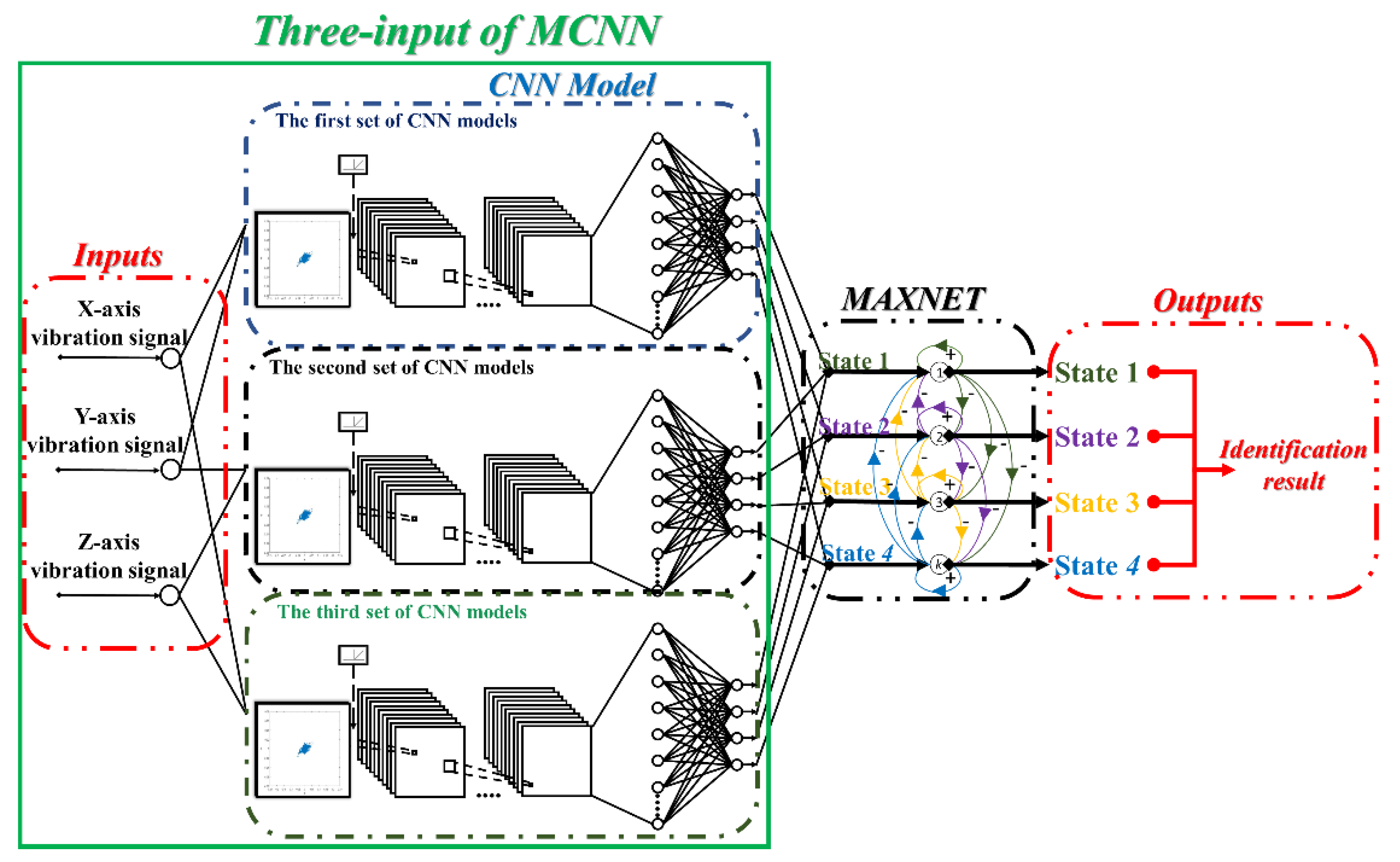
3.2.1. MCNN Architecture

The MCNN-based modeling proposed in this paper is an improvement over CNN through the integration of multiple CNN models. It executes troubleshooting based on different input data. Its architecture can be divided into three parts. Part 1 is the input layer, where different types of data are imported into the algorithm, and multiple signal characteristic diagrams are automatically generated. Part 2 involves identification and diagnosis, in which different types of designed signal characteristic diagrams are employed to train CNN models. The architecture of the network model mainly comprises multiple convolutional layers, pooling layers, fully connected layers, and activating layers. Lastly, Part 3 involves diagnosis result classification. In this paper, multiple signal characteristic diagrams generated on the front end were imported into the trained CNN models for identification. The identification results of these models were then summarized by the system, and MAXNET calculated the most accurate identification result.

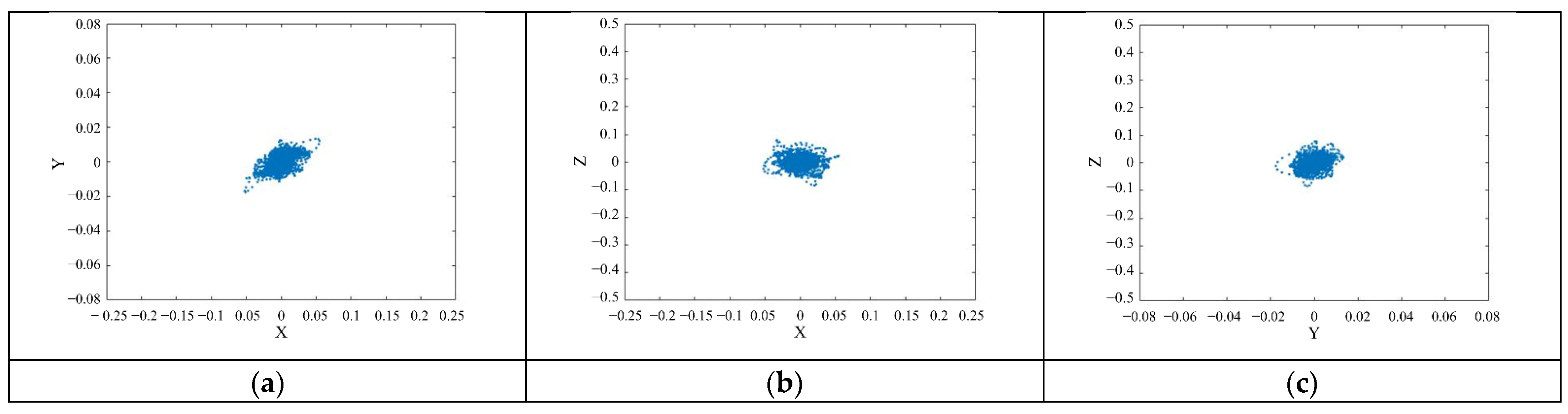
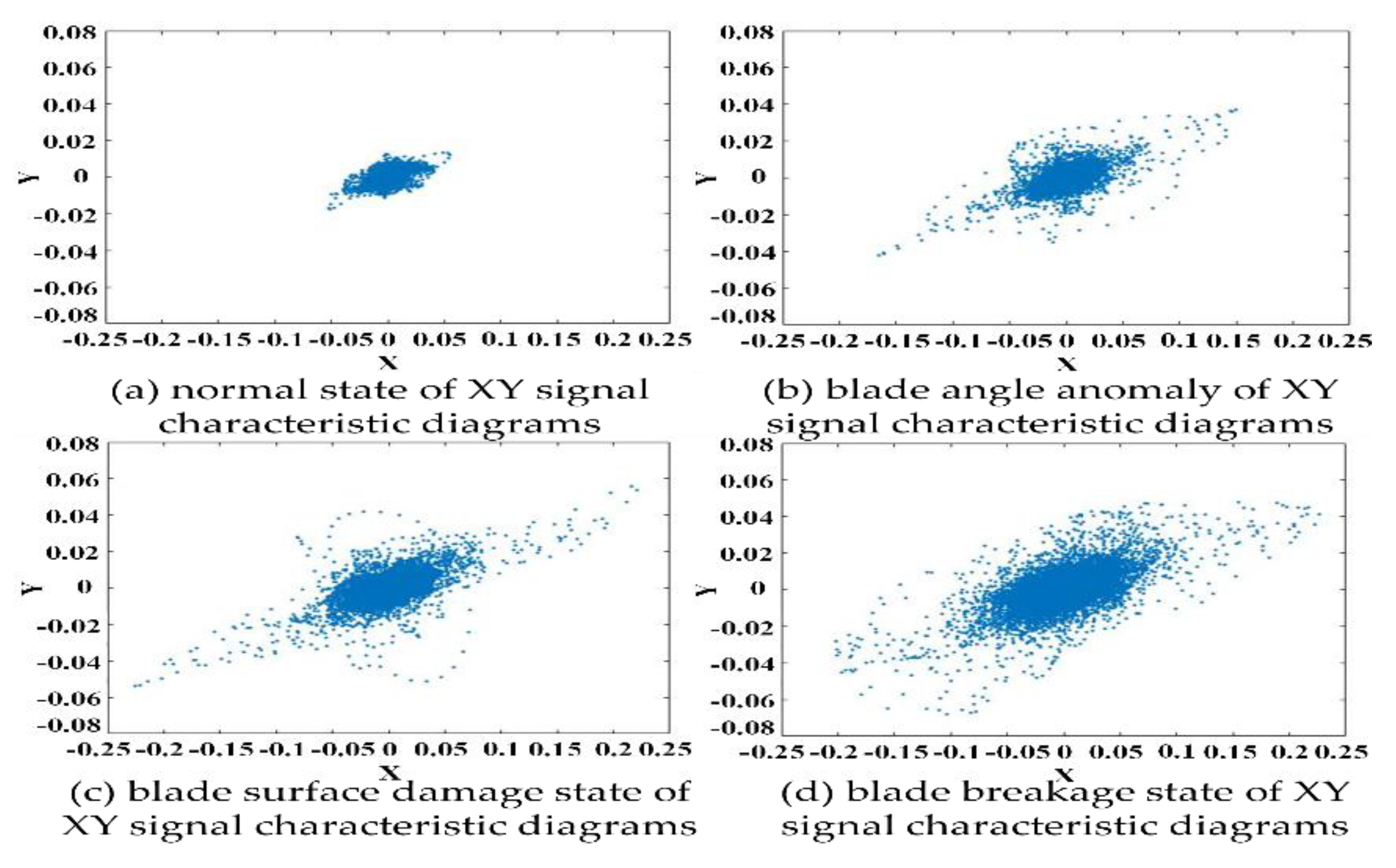
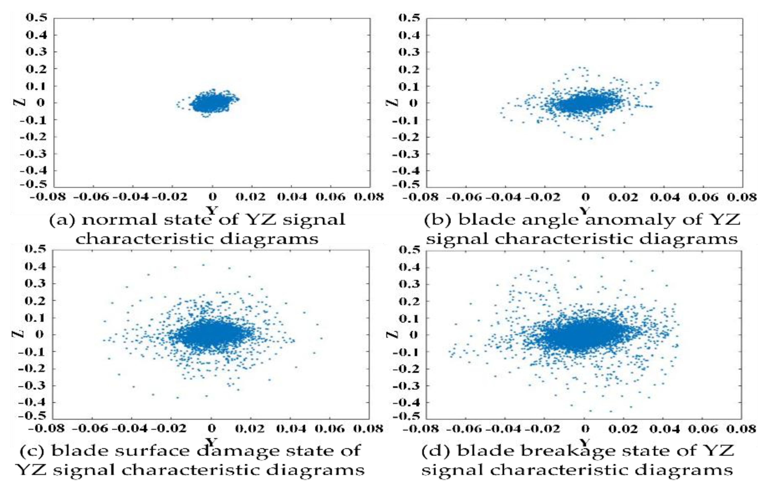
3.2.2. Signal Characteristic Diagrams of MCNN

The proposed MCNN in this study is a neural network developed for multiple types of inputs. Captured signals are filtered by the back-end signal processing unit before being imported. First, the data of the original signals of each axis are imported into the MCNN, which then identifies the data types and generates a corresponding type of signal characteristic diagram, as shown in Figure 10. Figure 10a shows the signal characteristic diagram after the data of the original signals of the X-axis and Y-axis are imported into the MCNN. Figure 10b shows the signal characteristic diagram after the data of the original signals of the X-axis and Z-axis are imported into the MCNN. Figure 10c shows the signal characteristic diagram after the data of the original signals of the Y-axis and Z-axis are imported into the MCNN. Lastly, different types of signal characteristic diagrams are learned and identified and signal characteristic diagrams of different types corresponding to the number of imported data types can be generated. The number of types of signal characteristic diagrams to be generated by the system is calculated in Equation (1):

$$\mathrm{N}={\complement }_2^{\mathrm{w}}=\frac{\mathrm{w}!}{2!\left(\mathrm{w}-2\right)!} \left(\mathrm{w}\ge 2\right)$$

(1)

where N represents the number of types of signal characteristic diagrams; w represents the number of input data types.

Therefore, the original signals measured by the three axes (X-axis, Y-axis, and Z-axis) are input into the MCNN and calculated by Equation (1) to obtain the paired data (X-axis and Y-axis, X-axis and Z-axis, and Y-axis and Z-axis). The original signals of any two kinds of data are then input into the same single image by the plot command of MATLAB, and the signal characteristic diagrams are drawn, as shown in Figure 10.

3.2.3. MCNN Diagnosis Result Classifier

The diagnosis result classifier adopted in this paper was the adaptive resonance theory (ART) artificial neural network [35]. At the input layer of the ART network, the identification results of multiple CNN models are imported. Input data is sent to the output layer through the neural population and weights. On the other hand, the ART output layer employs a maximum output network (MAXNET). Neurons on the ART output layer feed their respective signals back to enhance their signals while sending a signal that can relatively suppress other neurons. Through the competition in the network, the output layer can diagnose the most accurate fault type. MAXNET is a single-layer artificial neural network proposed by Lippmann in 1987 that can inhibit the feedback structure, and it has a lateral inhibition mechanism that uses a neuron (each value to be input for comparison) to inhibit other neurons. In this paper, the original measurement signals measured by the three axes (X-axis, Y-axis, and Z-axis) were input into the MCNN and calculated by Equation (1) to obtain three sets of data (X-axis and Y-axis, X-axis and Z-axis, and Y-axis and Z-axis). There were three CNN models, and the identification results of these CNN models were input to MAXNET for lateral inhibition calculation [36], as shown in Equation (2), in order to select and determine the final output identification results. Next, the original blade vibration signals that were actually measured at the wind field could be input into the trained MCNN model for identification.

$$W_{ij}=\{\begin{array}{c}1, i=j\\ -\epsilon , i\ne j,\end{array} \begin{array}{c} \\ \epsilon <1/M, and i\ge 1, j\le M\end{array}$$

(2)

where $W_{ij}$ is the weight of MAXNET; i and j are nodes of MAXNET; M is the number of classes, and all weights from each node to itself are 1. Weights between nodes are inhibitory, with a value of −ε where ε < 1/M.

4. Results

4.1. Wind Turbine Blade and Blade Angle Signal Measurement

In this paper, the wind turbine blade states included normal, blade angle anomaly, blade surface damage, and blade breakage. During state detection, the wind turbine blades rotated at a speed of 12 RPM. Vibration signals were measured every 50 ms. The sampled frequency was 51.2 kS/s. Each set of data had a length of 51,200 points, and 250 sets of data of the vibration signals for each of the four blade state types were measured and obtained. The vibration signal and the different faults are shown in

Table 2. The vibration signal and the different fault types.

Fault Type	Description
State 1	Normal wind turbine blades (The angle of each blade is 30°)
State 2	Blade angle anomaly (One of the blades has an angle of 45°)
State 3	A blade suffering a lightning strike (Surface damages at an 8.4 cm position)
State 4	Broken blade (The 8.4 cm front part of a blade was cut off)
Vibration Signal Information	Description
Wind turbine operation speed	12 RPM
Vibration signal acquisition time	50 millisecond
Sampling frequency	51.2 kS/s

. Therefore, a total of 1000 sets of data were obtained. The wind turbine signals were measured using a triaxial vibration transducer with a high-speed data capture card and were filtered by a signal processing unit. The filtered signal data were imported into the MCNN for learning and identification. Figure 11, Figure 12, Figure 13 and Figure 14 show the original vibration signals generated during the running of the wind turbine blades and the vibration signals filtered by the signal processing unit.

4.1.1. Model of the Turbine Blades in the Normal State

Figure 11 shows the triaxial vibration signals in the normal state. Normally, slight vibrations would occur during the running of the engine room. Therefore, the measured signals indicated that the wind turbine was in its normal state.

4.1.2. Model of the Wind Turbine Blades in the Blade Angle Anomaly State

Figure 12 shows the triaxial vibration signals in the blade angle anomaly state. By comparing the signals with those in the normal state, it could be found that the vibration signals on the X-axis greatly varied with the signals on the other two axes. The measured highest vibration amplitude was about 0.15 G.

4.1.3. Model of the Wind Turbine Blades in the Blade Surface Damage State

Figure 13 shows the triaxial vibration signals in the blade surface damage state. It could be found that the vibration signals on the Z-axis greatly varied with the signals on the other two axes. The measured highest vibration amplitude was about 0.38 G.

4.1.4. Model of the Large Wind Turbine Blades in the Blade Breakage State

Figure 14 shows the triaxial vibration signals in the blade breakage state. It could be found that the vibration signals on the Z-axis greatly varied with the signals on the other two axes. The measured highest vibration amplitude was about 0.48 G.

4.2. MCNN Identification System

This paper proposed the MCNN algorithm, which was an improvement over CNN as it could read the vibration signals on the X-axis, Y-axis, and Z-axis at the same time for learning and identification. A total of 3000 sets of vibration data were generated during the running of the measured wind turbine blades. The X-axis, Y-axis, and Z-axis accounted for 1000 sets of data, respectively. Each axis had four blade state types, and each type had 250 sets of data. First, the triaxial vibration signals were imported into the MCNN to generate three types of signal characteristic diagrams: XY, XZ, and YZ. Each type had 250 signal characteristic diagrams. For each type, 150 diagrams were randomly selected for training, and the remaining 100 were employed as test samples for MCNN learning and identification. The following explains the signal characteristic diagrams and identification results.

4.2.1. Signal Characteristic Diagrams of MCNN

Vibration signals were measured in four wind turbine blade models during the running of the wind turbines and were then captured and filtered by the back-end signal processing unit. Then, the X-axis, Y-axis, and Z-axis data were imported into the MCNN to generate three types of signal characteristic diagrams (XY, YZ, XZ), as shown in Figure 15, Figure 16 and Figure 17. By observing the signal characteristic diagrams generated in different wind turbine blade states, it could be found that the points on the signal characteristic diagrams of different states were dispersed in different positions and at different densities. Therefore, based on this feature, MCNN was applied for training and identification.

4.2.2. MCNN Identification Results

To train CNN models suitable for identifying the wind turbine blade state and blade angle, this paper adopted the XY, YZ, and XZ signal characteristic diagrams generated by MCNN to determine the optimal CNN model for each type through different numbers of layers, convolution kernel sizes, the activation function, and the pooling method. Then, the three models were integrated into the MCNN model. The test environment was MATLAB 2019b with an Intel Core (TM) i7-9700 [email protected] processor, an NVIDIA GeForce RTX 2080 SUPER graphics card, and the Windows 10 operating system.

Figure 18 shows the MCNN model designed in this paper for wind turbine blade state identification. There were a total of three CNN models, and each model had five convolutional layers, five pooling layers, one fully connected layer, the ReLu activation function, and max pooling. The three CNN models only had different convolution kernel sizes. CNN model 1 had a 3 × 3 convolution kernel size, CNN model 2 had a 1 × 1 convolution kernel size, and CNN model 3 had a 7 × 7 convolution kernel size. Lastly, the three models were integrated into the MCNN model and used for wind turbine troubleshooting, and the results showed it had up to an 87.8% identification accuracy.

The original signals measured by the three axes were input into the MCNN to gain the paired data and CNN models, and the identification results of these CNN models were input to MAXNET for lateral inhibition calculation to determine the final output results. According to the test results of this study, the recognition accuracy rate of the proposed method was as high as 87.8% after filtering, whereas the recognition accuracy of the original signal without filtering was only 81.3%, meaning that the filtering signals performed better at enhancing recognition accuracy. In this study, the filtering signals were be used for analysis. As listed in

Table 3. Comparison of recognition performance between MCNN and traditional detection methods.

Methods	Vibration Signals (axis)	Training Time (second)	Accuracy (%)	Average Accuracy (%)	Recognition Time (second)	Average Recognition Time (second)
MCNN	X, Y, Z	100	87.8	87.8	2.02	2.02
CNN	X, Y	100	86	84	1.56	1.73
CNN	X, Z	100	82		1.69
CNN	Y, Z	100	84		1.95
HOG+BPNN	X, Y	10,000	77.5	64.92	1.02	1.01
HOG+BPNN	X, Z	10,000	52		1
HOG+BPNN	Y, Z	10,000	65.25		1
HOG+SVM	X, Y	X	78.75	77.83	3.36	3.21
HOG+SVM	X, Z	X	77.25		2.94
HOG+SVM	Y, Z	X	78		3.32
HOG+KNN	X, Y	X	77.5	77.5	2.95	2.98
HOG+KNN	X, Z	X	78		2.92
HOG+KNN	Y, Z	X	77		3.08

, after the three types of signal characteristic diagrams were imported into the MCNN for identification, the identification accuracy reached up to 87.8%, representing the highest level using this approach. The accuracy for the XY vibration signals in CNN was 86%, while that for the XZ vibration signals was 82%. The accuracy for YZ vibration signals in CNN was 84%. In addition, this paper used HOG with BPNN, SVM, and KNN for image feature extraction and identification. For HOG+BPNN (XY, XZ, and YZ), the recognition accuracy was 77.5%, 52%, and 65.25%, respectively. For HOG+SVM (XY, XZ, and YZ), the recognition accuracy was 78.75%, 77.25%, and 78%, respectively. For HOG+KNN (XY, XZ, and YZ), the recognition accuracy was 77.5%, 78%, and 77%, respectively. In terms of the average recognition accuracy, MCNN had an 87.8% average recognition accuracy, which was the highest among these detection methods, followed by 91.9% for CNN, 77.83% for HOG+SVM, 77.5% for HOG+KNN, and 64.92% for HOG+BPNN. Regarding the average recognition time, while traditional CNN and HOG+BPNN could both quickly complete classifier training, CNN could complete the average recognition time in 1.73 s, while HOG+BPNN required only 1.01 s to complete the recognition, which was the fastest among these methods. HOG+KNN and HOG+ SVM could respectively complete the recognition in 2.98 s and 3.21 s, which was the most time-consuming. MCNN required 2.02 s to complete the recognition. In view of the above, the accuracy of using traditional detection methods and CNN was below that of MCNN. Therefore, for the blade states detected in this paper, vibration signals must be detected on three axes instead of only one. The proposed algorithm not only had the highest accuracy compared with the traditional methods but also required only 2.02 s for identification.

The recognition result of wind turbine blades is displayed in a confusion matrix, as shown in Figure 19, where the x-axis is the actual fault type, and the y-axis is the predicted fault type. The green and red grids of the confusion matrix indicate the number of accurate recognitions and the number of misrecognitions, respectively. Among the 100-test data of type 3, the proposed method identified 71 data as type 3, 1 data as type 2, and 28 data as type 4, so the recognition rate of type 3 was 71%. Similarly, the recognition of type 1 and type 4 of the proposed method were all 100%, and that of Type 2 was 80%. Finally, the value of green grids was divided by the sum of the green and red grid values, and the total recognition accuracy rate was 87.8%.

5. Conclusions

This paper developed a wind turbine blade and blade angle troubleshooting system, which can be applied to intelligent wind turbine blade state detection. Further, this paper selected three common blade and blade angle fault types according to the statistics of prior studies. Models were built based on the normal state and the three faulty states. Signals measured on any two axes of a triaxial vibration transducer were combined and adopted to generate signal characteristic diagrams. Meanwhile, signals measured on any axis of a triaxial vibration transducer were imported into CNN. By comparing the identification accuracy of the two, it was found that the proposed approach had an accuracy up to 87.8%, demonstrating that it can be adopted for effective troubleshooting of wind turbine blade and blade angle. In the future, the proposed approach could also be applied in other electric power and energy-related fields, such as generators, bearings, gearboxes, power capacitors, gas-insulated switchgear (GIS) switches, lightning arrestors, transformers, and motors.

References

1. Pu, Z.; Li, C.; Zhang, S.; Bai, Y. Fault Diagnosis for Wind Turbine Gearboxes by Using Deep Enhanced Fusion Network. IEEE Trans. Instrum. Meas. 2021, 70, 1–11. [Google Scholar] [CrossRef]
2. He, Q.; Zhao, J.; Jiang, G.; Xie, P. An Unsupervised Multiview Sparse Filtering Approach for Current-Based Wind Turbine Gearbox Fault Diagnosis. IEEE Trans. Instrum. Meas. 2020, 69, 5569–5578. [Google Scholar] [CrossRef]
3. Wang, J.; Qiao, W.; Qu, L. Wind Turbine Bearing Fault Diagnosis Based on Sparse Representation of Condition Monitoring Signals. IEEE Trans. Ind. Appl. 2019, 55, 1844–1852. [Google Scholar] [CrossRef]
4. Huang, N.; Chen, Q.; Cai, G.; Xu, D.; Zhang, L.; Zhao, W. Fault Diagnosis of Bearing in Wind Turbine Gearbox Under Actual Operating Conditions Driven by Limited Data With Noise Labels. IEEE Trans. Instrum. Meas. 2021, 70, 1–10. [Google Scholar] [CrossRef]
5. Liu, Z.; Tang, X.; Wang, X.; Mugica, J.E.; Zhang, L. Wind Turbine Blade Bearing Fault Diagnosis Under Fluctuating Speed Operations via Bayesian Augmented Lagrangian Analysis. IEEE Trans. Ind. Inform. 2021, 17, 4613–4623. [Google Scholar] [CrossRef]
6. Shi, Z.F.; Liu, J.; Li, H.W.; Zhang, Q.; Xiao, G.J. Dynamic simulation of a planet roller bearing considering the cage bridge crack. Eng. Fail. Anal. 2022, 131, 105849. [Google Scholar] [CrossRef]
7. Liu, J.; Xu, Z.D. A simulation investigation of lubricating characteristics for a cylindrical roller bearing of a high-power gearbox. Tribol. Int. 2022, 167, 107373. [Google Scholar] [CrossRef]
8. Ibrahim, R.K.; Watson, S.J.; Djurović, S.; Crabtree, C.J. An Effective Approach for Rotor Electrical Asymmetry Detection in Wind Turbine DFIGs. IEEE Trans. Ind. Electron. 2018, 65, 8872–8881. [Google Scholar] [CrossRef] [Green Version]
9. Artigao, E.; Honrubia-Escribano, A.; Gómez-Lázaro, E. In-Service Wind Turbine DFIG Diagnosis Using Current Signature Analysis. IEEE Trans. Ind. Electron. 2020, 67, 2262–2271. [Google Scholar] [CrossRef]
10. Oh, K.-Y.; Park, J.-Y.; Lee, J.-S.; Epureanu, B.I.; Lee, J.-K. A Novel Method and Its Field Tests for Monitoring and Diagnosing Blade Health for Wind Turbines. IEEE Trans. Instrum. Meas. 2015, 64, 1726–1733. [Google Scholar] [CrossRef]
11. Liu, Z.; Wang, X.; Zhang, L. Fault Diagnosis of Industrial Wind Turbine Blade Bearing Using Acoustic Emission Analysis. IEEE Trans. Instrum. Meas. 2020, 69, 6630–6639. [Google Scholar] [CrossRef]
12. Malik, H.; Mishra, S. Artificial neural network and empirical mode decomposition based imbalance fault diagnosis of wind turbine using TurbSim, FAST and Simulink. IET Renew. Power Gener. 2017, 11, 889–902. [Google Scholar] [CrossRef]
13. Yang, J.; Zhao, L.; Lang, Z.-Q.; Zhang, Y. Wind Turbine Blade Condition Monitoring and Damage Detection by Image-Based Method and Frequency-Based Analysis. In Proceedings of the 2018 10th International Conference on Modelling, Identification and Control (ICMIC), Guiyang, China, 2–4 July 2018; pp. 1–6. [Google Scholar]
14. Sahoo, S.; Kushwah, K.; Sunaniya, A.K. Health Monitoring of Wind Turbine Blades through Vibration Signal Using Advanced Signal Processing Techniques. In Proceedings of the 2020 Advanced Communication Technologies and Signal Processing (ACTS), Silchar, India, 4–6 December 2020; pp. 1–6. [Google Scholar]
15. Liu, X.; Zhang, X.; Wang, L. Fault Diagnosis Method of Wind Turbine Gearbox Based on Deep Belief Network and Vibration Signal. In Proceedings of the 2018 IEEE 57th Annual Conference of the Society of Instrument and Control Engineers of Japan (SICE), Nara, Japan, 11–14 September 2018; pp. 1699–1704. [Google Scholar]
16. Yu, X.; Tang, B.; Zhang, K. Fault Diagnosis of Wind Turbine Gearbox Using a Novel Method of Fast Deep Graph Convolutional Networks. IEEE Trans. Instrum. Meas. 2021, 70, 1–14. [Google Scholar] [CrossRef]
17. Firuzi, K.; Vakilian, M.; Phung, B.T.; Blackburn, T.R. Partial Discharges Pattern Recognition of Transformer Defect Model by LBP & HOG Features. IEEE Trans. Power Deliv. 2019, 34, 542–550. [Google Scholar]
18. Hu, J.; Kuang, Y.; Liao, B.; Cao, L.; Dong, S.; Li, P. A Multichannel 2D Convolutional Neural Network Model for Task-Evoked fMRI Data Classification. Comput. Intell. Neurosci 2019, 2019, 5065214. [Google Scholar] [CrossRef] [PubMed]
19. Schwenk, H.; Bengio, Y. Training methods for adaptive boosting of neural networks for character recognition. In Advances in Neural Information Processing Systems 10: Proceedings of the 1997 Conference; The MIT Press: Cambridge, MA, USA, 1998; pp. 647–653. [Google Scholar]
20. Saghafinia, A.; Kahourzade, S.; Mahmoudi, A.; Hew, W.P.; Uddin, M.N. On line trained fuzzy logic and adaptive continuous wavelet transform based high precision fault detection of IM with broken rotor bars. In Proceedings of the 2012 IEEE Industry Applications Society Annual Meeting, Las Vegas, NV, USA, 7–11 October 2012; pp. 1–8. [Google Scholar]
21. Saucedo-Dorantes, J.J.; Arellano-Espitia, F.; Delgado-Prieto, M.; Osornio-Rios, R.A. Diagnosis Methodology Based on Deep Feature Learning for Fault Identification in Metallic, Hybrid and Ceramic Bearings. Sensors 2021, 21, 5832. [Google Scholar] [CrossRef]
22. Jiang, G.; He, H.; Xie, P.; Tang, Y. Stacked Multilevel-Denoising Autoencoders: A New Representation Learning Approach for Wind Turbine Gearbox Fault Diagnosis. IEEE Trans. Instrum. Meas. 2017, 66, 2391–2402. [Google Scholar] [CrossRef]
23. Dao, C.; Kazemtabrizi, B.; Crabtree, C. Wind turbine reliability data review and impacts on levelised cost of energy. Wind Energy 2019, 22, 1848–1871. [Google Scholar] [CrossRef] [Green Version]
24. Pao, L.Y.; Johnson, K.E. Control of Wind Turbines. IEEE Control Syst. Mag. 2011, 31, 44–62. [Google Scholar]
25. Qiao, W.; Lu, D. A Survey on Wind Turbine Condition Monitoring and Fault Diagnosis—Part I: Components and Subsystems. IEEE Trans. Ind. Electron. 2015, 62, 6536–6545. [Google Scholar] [CrossRef]
26. Chou, J.-S.; Chiu, C.-K.; Huang, I.-K.; Chi, K.-N. Failure Analysis of Wind Turbine Blade under Critical Wind Loads. Eng. Fail. Anal. 2013, 27, 99–118. [Google Scholar] [CrossRef]
27. Wilson, N.; Myers, J.; Cummins, K.L.; Hutchinson, M.; Nag, A. Lightning Attachment to Wind Turbines in Central Kansas: Video Observations Correlation with The NLDN and In-situ Peak Current Measurements. In Proceedings of the European Wind Energy Association Annual Event, Vienna, Austria, 4–7 February 2013; pp. 1–8. [Google Scholar]
28. Cummins, K.L.; Qucik, M.G.; Rison, W.; Krehbiel, P.; Thomas, R.; Mcharg, G.; Engle, J.; Myers, J.; Nag, A.; Cramer, J.; et al. Overview of the Kansas Windfarm2013 Field Program. In Proceedings of the 23rd International Lightning Detection Conference, Tucson, AZ, USA, 18–19 March 2014. [Google Scholar]
29. IEC 61400-24 Ed.1.0. Wind Turbines–Part 24: Lightning Protection. 2010. IEC: Geneva, Switzerland, 2010.
30. Garolera, A.C.; Madsen, S.F.; Nissim, M.; Myers, J.D.; Holboell, J. Lightning Damage to Wind Turbine Blades From Wind Farms in the U.S. IEEE Trans. Power Delivery 2016, 31, 1043–1049. [Google Scholar] [CrossRef]
31. Ranjan, R.; Bansal, A.; Zheng, J.; Xu, H.; Gleason, J.; Lu, B.; Nanduri, A.; Chen, J.C.; Castillo, C.D.; Chellappa, R. A Fast and Accurate System for Face Detection, Identification, and Verification. IEEE Trans. Biom. Behav. Identity Sci. 2019, 1, 82–96. [Google Scholar] [CrossRef] [Green Version]
32. Pereira, S.; Pinto, A.; Alves, V.; Silva, C.A. Brain Tumor Segmentation Using Convolutional Neural Networks in MRI Images. IEEE Trans. Med. Imaging 2016, 35, 1240–1251. [Google Scholar] [CrossRef]
33. Liu, R.; Meng, G.; Yang, B.; Sun, C.; Chen, X. Dislocated Time Series Convolutional Neural Architecture: An Intelligent Fault Diagnosis Approach for Electric Machine. IEEE Trans. Ind. Inform. 2017, 13, 1310–1320. [Google Scholar] [CrossRef]
34. Lecun, Y.; Bottou, L.; Bengio, Y.; Haffner, P. Gradient-Based Learning Applied to Document Recognition. Proc. IEEE 1998, 86, 2278–2324. [Google Scholar] [CrossRef] [Green Version]
35. Wong, S.Y.; Yap, K.S.; Lim, C.P.; Lee, E.W.M. Hybrid Data Regression Model Based on the Generalized Adaptive Resonance Theory Neural Network. IEEE Access 2019, 7, 116438–116452. [Google Scholar] [CrossRef]
36. Lippmann, R. An introduction to computing with neural nets. IEEE ASSP Mag. 1987, 4, 4–22. [Google Scholar] [CrossRef]
Figure 1. Architecture of the proposed system.
Sustainability 14 01781 g001
Figure 2. Human-machine interface for vibration analysis and detection.
Sustainability 14 01781 g002
Figure 3. The wind turbine blades adopted in this paper.
Sustainability 14 01781 g003
Figure 4. Normal wind turbine blade model (state 1).
Sustainability 14 01781 g004
Figure 5. Blade angle anomaly model (State 2).
Sustainability 14 01781 g005
Figure 6. Blade surface damage model (State 3).
Sustainability 14 01781 g006
Figure 7. Broken blade model (State 4).
Sustainability 14 01781 g007
Figure 8. The wind turbine fault diagnosis process.
Sustainability 14 01781 g008
Figure 9. The overall LeNet architecture (CNN).
Sustainability 14 01781 g009
Figure 10. Signal characteristic diagrams generated by MCNN for each axis. (a) Signal characteristic diagram for the X-axis and Y-axis; (b) Signal characteristic diagram for the X-axis and Z-axis; (c) Signal characteristic diagram for the Y-axis and Z-axis.
Sustainability 14 01781 g010
Figure 11. Vibration signals of the wind turbine blades in the normal state.
Sustainability 14 01781 g011
Figure 12. Vibration signals of the wind turbine blades in the blade angle anomaly state.
Sustainability 14 01781 g012
Figure 13. Vibration signals of the large wind turbine blades in the blade surface damage state.
Sustainability 14 01781 g013
Figure 14. Vibration signals in the blade breakage state.
Sustainability 14 01781 g014
Figure 15. XY signal characteristic diagrams of wind turbine blades.
Sustainability 14 01781 g015
Figure 16. XZ signal characteristic diagrams of wind turbine blades.
Sustainability 14 01781 g016
Figure 17. YZ signal characteristic diagrams of wind turbine blades.
Sustainability 14 01781 g017
Figure 18. The MCNN architecture proposed in this paper.
Sustainability 14 01781 g018
Figure 19. Confusion matrixes of MCNN for fault detection of wind turbine blades.
Sustainability 14 01781 g019