A Fuzzy-Interval Dynamic Optimization Model for Regional Water Resources Allocation under Uncertainty

Abstract

In this study, a fuzzy-interval dynamic programming (FIDP) model is proposed for regional water management under uncertainty by combining fuzzy-interval linear programming (FILP) and dynamic programming (DP). This model can not only tackle uncertainties presented as intervals, but also consider the dynamic characteristics in the allocation process for water resources. Meanwhile, the overall satisfaction from users is considered in the objective function to solve the conflict caused by uneven distribution of resources. The FIDP model is then applied to the case study in terms of water resources allocation under uncertainty and dynamics for the City of Handan in Hebei Province, China. The obtained solutions can provide detailed allocation schemes and water shortage rates at different stages. The calculated comprehensive benefits of economy, water users’ satisfaction and pollutant discharge (i.e., COD) are [2264.72, 2989.33] × 10⁸ yuan, [87.50, 96.50] % and [1.23, 1.65] × 10⁸ kg respectively with a plausibility degree (i.e., ${\lambda }_{opt}^{\pm }$) ranging within [0.985, 0.993]. Moreover, the benefit from FIDP model under consideration of dynamic features is more specific and accurate than that of FILP model, whilst the water shortage rate from FIDP is [5.10, 9.10] % lower than that of FILP model.

1. Introduction

Due to population growth, economic development and consumption upgrade, global water consumption has increased by six times, and it has been continuing to grow steadily at an annual rate of about 1% during the past 100 years [1]. All of these would lead to the water shortage problem that is already pessimistically even severer, and seriously hinders the sustainable development of social economy. Managing water resources is an effective way to deal with the above challenges. However, in the process of management, experts and governors have encountered a lot of problems [2,3,4,5,6], such as dynamic variability and uncertainty, which are thorny and inevitable. Besides, in areas with water shortage, when the available water cannot meet the needs, unreasonable water allocation will lead to conflicts among users [7]. Therefore, it is definitely necessary to put forward a comprehensive model to deal with dynamic variabilities and uncertainties in water resources system as well as the contradiction between different users, so as to improve the management efficiency and the users’ satisfaction.

The water resources system is of great complexities involving many uncertain factors, such as water use efficiency, water demand, pollutant discharge, water supply capacity and so on, and these uncertain factors could affect the structure for the optimal allocation model of water resources and resulting solutions [8,9,10,11]. Previously, scholars in related fields have got fruitful achievements in dealing with uncertainties in water resources management. For the optimization under uncertainties, mathematical methods that are commonly used include stochastic programming [12], fuzzy programming [13], interval programming [14], and various coupling programming methods [15]. Among them, fuzzy programming can deal with the conflicts among multi-objective functions well, making it a new flexible planning problem [16], while the interval programming can reflect the uncertain coefficients in the form of intervals, and convert the uncertain planning problems into deterministic planning problems [17]. Both of them are helpful to solve uncertain planning problems. Based on these models, a large number of integrated models have been developed to optimize the allocation of water resources, such as uncertain two-stage stochastic water resources optimal allocation model [18], improved interval linear optimal allocation model [19], chance constrained water resources optimal allocation model [20], multi-objective interval linear water resources optimal allocation model [21], and so on [22,23,24]. Li et al. [25] proposed a multi-objective water resources optimal allocation model under uncertainties by integrating constrained programming, semi-infinite programming, integer programming and interval linear programming. Suo et al. [26] presented an approach for interval multi-objective planning by coupling fuzzy programming and improved two-step method, and then proved the objectivity and stability of this method by comparing it with the weighted sum method. Li et al. [27] formulated a new two-stage random interval parameter fuzzy planning strategy model by considering various uncertainties in planning and management of water resources and water environment systems, which was then applied to reveal the relationship between local economic goals and environmental goals. The above-mentioned models can well deal with the uncertainty in data acquisition in the system. However, they are insufficient to handle the dynamic features in the allocation process of water resources.

In the process of water resources optimization, it is essential to give a full consideration to dynamic characteristics, and thus provide the best scheme for water distribution at different stages of the planning period [28]. Dynamic programming cannot only solve the optimization problem of multi-stage decision process in water resources allocation [29], but also obtain the optimal strategy of the whole process and the optimal sub-strategy of each stage [30,31,32,33,34]. Peng [35] established a multi-objective dynamic water resources allocation model to achieve a dynamic balance for the optimal water resources allocation by using a modified simplex method with the addition of a time variable. Feng [36] set up a multi-objective dynamic water resources optimization configuration model and introduced the satisfaction function to realize the dynamic balance of optimal allocation of water resources on the time scale. Ramírez et al. [37] used stochastic dynamic programming to provide release decisions for each stage, and combined genetic algorithm and reservoir operation simulation program to obtain the annual release curve. These models proposed above are able to solve the multi-stage decision-making problem and get satisfactory allocation results. However, they took less consideration for uncertainties in water resources system.

Therefore, in order to comprehensively consider uncertainties and dynamic variability in the water resources system, a fuzzy-interval dynamic (FIDP) optimal allocation model is proposed in this study by integrating fuzzy-interval linear programming (FILP) and dynamic programming (DP) into a general framework. In addition, in order to realize the fairness of water resources allocation, the satisfaction function is added as one objective function to reduce the contradictions among users. The main innovative points of this study can be summarized as: (i) By introducing FILP into the FIDP model, the uncertainty coefficients and constraints, such as water use efficiency and water demand in water resources system, can be reflected in the form of interval numbers, which would make the results more accurate and reasonable. (ii) By introducing DP into FIDP model, not only the annual optimization scheme, but also the detailed water distribution scheme of each stage in planning year can be obtained. (iii) For FIDP model, the principle of fairness for water users is added to the objective function, which can reduce the contradictions between government and water users, as well as among different water users. This model is then applied to Handan City, Hebei Province, China, where water volume is small and uneven, to pursue the maximization for social benefits, overall satisfaction of water users, and environmental benefits. Finally, the FIDP model is compared with the traditional FILP model, to prove the dynamic superiority of the proposed model with stage changes. It is expected that this model would be helpful to optimize the allocation of regional water resources under uncertainties and dynamics to reduce water shortage and conflict, and promote sustainable development of local society and economy.

This paper is composed of the following parts. Section 2 expounds the generation process of the general FIDP method. Section 3 puts forward a specific FIDP model suitable for Handan city. Section 4 presents the result analysis, which briefly expounds the water consumption characteristics of users at different stages of the planning year, and then compares the proposed FIDP model with FILP model. Section 5 is the summary of this study.

2. Methodology

2.1. Fuzzy-Interval Linear Programming (FILP)

On account of parameter uncertainties and objective inconsistency in multi-objective programming [38,39,40], the FILP model can well handle the uncertainty parameters denoted by interval numbers, and also coordinate the conflicts among different objective functions by introducing membership function λ, which makes the resulting solutions more scientific and reliable. The model is summarized as follows [26]:

$$Max{\lambda }^{\pm }$$

(1a)

Subject to:

$$C_g^{\pm }{X}^{\pm }\ge f_g^{-}+{\lambda }^{\pm }(f_g^{+}-f_g^{-})\hspace{0.5em}g=1,2, \dots , m$$

(1b)

$$C_h^{\pm }{X}^{\pm }\le f_h^{+}-{\lambda }^{\pm }(f_h^{+}-f_h^{-})\hspace{0.5em}h=m+1, \dots , n$$

(1c)

$$A_i^{\pm }{X}^{\pm }\le B_i^{\pm }\hspace{0.5em}i=1, 2, \dots , k$$

(1d)

$$X^{\pm }\ge 0$$

(1e)

$$0\le {\lambda }^{\pm }\le 1$$

(1f)

It is worth noting that:

$$C_g^{\pm }{X}^{\pm }=Max f_g^{\pm }\hspace{0.5em}g=1,2, \dots , m$$

(2a)

$$C_h^{\pm }{X}^{\pm }=Min f_h^{\pm }\hspace{0.5em}h=m+1, \cdots , n$$

(2b)

where $C_g^{\pm }\in {\left\{R_1^{\pm }\right\}}^{1\times t}$, $C_h^{\pm }\in {\left\{R_2^{\pm }\right\}}^{1\times t}$, $A_i^{\pm }\in {\left\{R_3^{\pm }\right\}}^{1\times t}$, $X^{\pm }\in {\left\{R_4^{\pm }\right\}}^{t\times 1}$, and $R_e^{\pm }$ means a set of interval numbers ($e\in [1, 2, 3, 4]$), g and h are core markers for maximizing and minimizing the objective functions individually, and i is the index of the constraints. $f^{-}$, $f^{+}$ are the lower and upper bounds of $f^{\pm }$, and ${\lambda }^{\pm }$ is the membership function in fuzzy decision-making. The larger the ${\lambda }^{\pm }$ is, the more credible the calculation result would be; on the contrary, the smaller ${\lambda }^{\pm }$ would lead to less credible results.

2.2. Dynamic Programming (DP)

The basic idea of dynamic programming is that it not only separates the current stage from the future stages, but also considers the current benefit and the future benefit together. Therefore, the optimal decision selection of each stage is from the overall consideration, which is generally different from the optimal choice of this stage [41]. Concretely, for a multi-stage decision-making problem, dynamic programming can divide it into several stages according to time or other characteristics, and each stage has several states and decision strategies [42]. The system transfers from one stage to the next according to a certain rule, and the purpose is to obtain the optimal strategy combining each stage [43]. The following Equation (3) is the state transition formula of dynamic programming, and it is also the most important part of dynamic programming.

$$S_j=T(S_{j-1}, x_{j-1})\hspace{0.5em}j=1, 2, \dots , l$$

(3)

where $S_j$ stands for the state variable at stage j, with l stages in total. $x_{j-1}$ represents the decision variable at stage $j-1$, and $T(S_{j-1}, x_{j-1})$ is the state transition function [44].

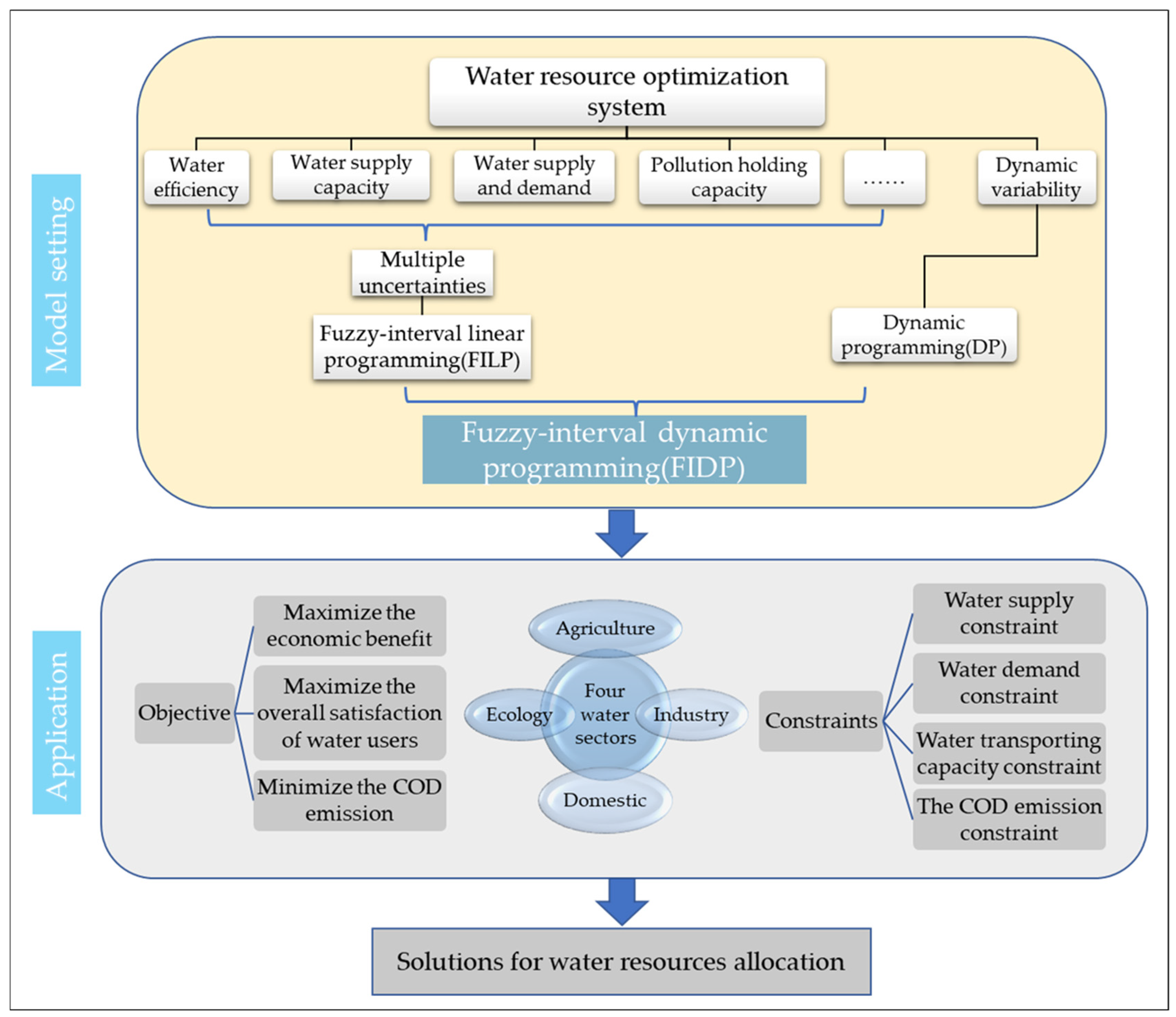
2.3. Fuzzy-Interval Dynamic Programming (FIDP)

It is noted that multiple uncertainties and dynamic variability exist in the water resources system, which seriously affect effective planning and management of water resources. Although FILP and DP can efficiently address interval uncertainty, coordinate conflicts among different objective functions and characterize systems’ dynamics individually, they are unable to deal with those problems at the same time. Therefore, this paper aims to propose a FIDP model by incorporating FILP and DP into one framework to comprehensively reflect both uncertainties and dynamic features in the water resources system. In addition, the function of the users’ satisfaction is considered to solve the contradiction caused by uneven distribution of resources. The developed model is shown as follows.

$$Max{\lambda }^{\pm }$$

(4a)

Subject to:

$$C_g^{\pm }{X}^{\pm }\ge f_g^{-}+{\lambda }^{\pm }(f_g^{+}-f_g^{-})\hspace{0.5em}g=1, 2, \dots , m$$

(4b)

$$\frac{X^{\pm }}{G^{\pm }}\alpha \ge f_p^{-}+{\lambda }^{\pm }(f_p^{+}-f_p^{-})\hspace{0.5em}p=m+1, m+2, \dots , r$$

(4c)

$$C_h^{\pm }{X}^{\pm }\le f_h^{+}-{\lambda }^{\pm }(f_h^{+}-f_h^{-})\hspace{0.5em}h=r+1, r+2, \dots , n$$

(4d)

$$A_i^{\pm }{X}^{\pm }\le B_i^{\pm }\hspace{0.5em}i=1, 2, \dots , k$$

(4e)

$$S_j^{\pm }=T(S_{j-1}^{\pm }, x_{j-1}^{\pm })\hspace{0.5em}j=1, 2, \dots , l$$

(4f)

$$A_j^{\pm }{X}^{\pm }\le S_j^{\pm }\hspace{0.5em}j=0, 1, \dots , l$$

(4g)

$$0\le X^{\pm }\le G^{\pm }$$

(4h)

$$S_0^{\pm }=0$$

(4i)

$$0\le {\lambda }^{\pm }\le 1$$

(4j)

where the symbol $G^{\pm }$ means the user’s ideal demand for resources, and α is the weight coefficient of different users. And Equation (4c) can reflect the fairness for different users, Equation (4f) realizes the dynamic transition, and the state constraint after phase transition is achieved by Equation (4g).

The steps of solving the FIDP model can be summarized as: (i) Establish FIDP model. (ii) Divide the model into two submodels through an improved two-step method [45]. In order to maximize ${\lambda }^{\pm }$, the upper bound submodel should be formulated firstly. (iii) Solve the upper bound submodel and obtain $x_{opt}^{+}$ and ${\lambda }_{opt}^{+}$. (iv) Formulate the lower bound submodel for the FIDP model. (v) Solve the lower bound and obtain $x_{opt}^{-}$ and ${\lambda }_{opt}^{-}$. (vi) According to the results of the above two models, the objective function values are calculated by formulate (2). (vii) Combining these two submodels, the optimal solution can be expressed as $f_{g opt}^{\pm }=[f_{g opt}^{-}, f_{g opt}^{+}]$ ($g=1, 2, \dots , m$), $f_{p opt}^{\pm }=[f_{p opt}^{-}, f_{p opt}^{+}]$ ($p=m+1, m+2, \dots , r$), $f_{h opt}^{\pm }=[f_{h opt}^{-}, f_{h opt}^{+}]$ ($h=r+1, r+2, \dots , n$), ${\lambda }_{opt}^{\pm }=[{\lambda }_{opt}^{-}, {\lambda }_{opt}^{+}]$, $X_{opt}^{\pm }=[X_{opt}^{-}, X_{opt}^{+}]$.

In general, the presented model can be applicable for the following problems: (i) For those problems with uncertain factors, this method can reflect them in model establishment, solution process and results in the form of interval numbers. (ii) For multi-stage decision-making problems, this model can provide specific schemes for every stage and global optimal solutions for the whole process. (iii) For multi-objective and multi-user problems, this model can coordinate the conflicts among different objective functions by maximizing satisfaction of the objective functions, and reduce the contradictions among users by considering the principle of fairness.

3. Case Study

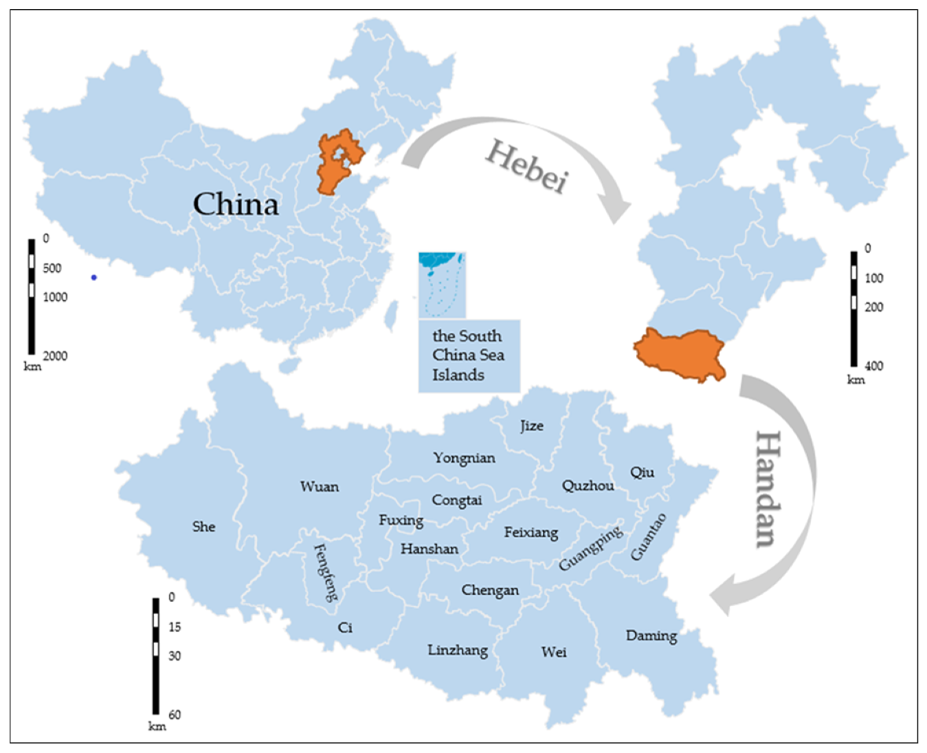
3.1. Overview of Handan City

The city of Handan is located in the southernmost part of Hebei Province, China, at the eastern foot of Taihang Mountain, bordering Shandong in the east, Henan in the south, Shanxi Province in the west and Xingtai City in the north. Its jurisdiction covers 6 districts, 1 county-level city and 11 counties. Its geographical location ranges 36°04′~37°01′ N and, 113°28′~115°28′ E with warm temperate semi-humid and semi-arid continental monsoon climate. The location of the area is shown in Figure 1.

At present, water resource managers in Handan are facing with many water resource problems, such as water resource shortage, uneven distribution of precipitation, and serious water pollution. For example, according to the Water Resources Bulletin [46], the per capita water consumption of the city in 2019 is 2.02 × 10² m³ with a population of 9.55 million. However, the water supply in 2019 is only 1927.84 × 10⁶ m³, and the water shortage is 1.26 × 10⁶ m³. In addition, 61.30%~76.50% of the annual precipitation falls between June and September, which is extremely inconsistent with the needs from various water users. Actually, each user’s water demand, especially the agricultural water demand, is different with the season changes. The growing period of crops in Handan mainly ranges from March to August, with the largest water demand occurring at the second stage which would account for about 50% of the annual water consumption. It is noted that the development of agricultural cultivation is paid the most attention in Handan City, and its water consumption accounts for about 55% of the total water consumption. So how to provide periodic water allocation for each user is a challenge for managers. Moreover, due to the uncertainties existing in water supply and the temporal variations of the planning horizon, the water resources system also has a number of uncertain factors, such as the water inflows at different stages, water efficiency, water demand, and pollutant discharge, which should be fully considered. Therefore, how to allocate water resources reasonably to ensure the sustainable development of this region is an urgent problem for managers to solve under condition of discordant water supply and demand, as well as various uncertain factors.

3.2. Application of FIDP Model

In order to primely solve the problems mentioned above, FIDP is applied to optimize the allocation of water resources in Handan city. In detail, the established FIDP model would not only considers multiple objectives, such as the maximum economic benefit, the maximum overall satisfaction of water users, and the maximum environmental benefit, but also take the satisfaction of each water users into account. Meanwhile, the constraints would refer to the water supply capacity, the minimum guaranteed water demand, the ideal water demand, the water delivery capacity, and the COD emission limit. In addition, the uncertain factors involved in this model (e.g., water use benefit coefficient, ideal water demand, minimum guaranteed water demand, weight coefficient, COD discharge coefficient, maximum COD discharge, available water supply, water inflow at different stages, and water delivery capacity) can be expressed as interval parameters. Moreover, the dynamic factors in the process of water resources optimization, such as the water users’ ideal water demand, guaranteed water demand, available water supply and water allocation changing with the stage, would be reflected by dynamic programming. The frame diagram of constructed FIDP model can be seen in Figure 2. In order to facilitate managers to make decisions, each stage is divided equally by the planning year, in which, January-March is the first stage, April-June is the second stage, the third stage is from July to September, and the fourth stage is from October to December. Its formulation would be expressed in the following form:

3.2.1. Objective Functions

The goal of this model is to maximize its membership function:

$$Max{\lambda }^{\pm }$$

(5a)

3.2.2. Constraints

Economic benefit constraint (maximize the economic benefit):

$${\displaystyle \sum _{t=1}^4{\displaystyle \sum _{i=1}^4{\displaystyle \sum _{j=1}^{16}{\displaystyle \sum _{k=1}^4{e}_{tjk}^{\pm }{a}_{tijk}{x}_{tijk}^{\pm }}}}}\ge f_1^{-}+{\lambda }^{\pm }(f_1^{+}-f_1^{-})$$

(5b)

where t denotes stage of the planning year ($t=1, 2, 3, 4$), i is water source ($i=1, 2, 3, 4$, representing surface water, underground water, diverted water and recycled water), j means region ($j=1, 2, 3, \dots , 16$, representing Urban, Wuan, Jize, Qiu, Quzhou, Guantao, She, Guangping, Chengan, Wei, Ci, Linzhang, Daming, Fengfeng, Yongnian and Feixiang), k stands for water user (k = 1, 2, 3, 4, representing agricultural, industrial, domestic and ecological), $e_{tijk}^{\pm }$ is net efficiency coefficient of water used by user k in region j in the t stage of planning year (yuan/m³), $a_{tijk}$ denotes water relationship provided by water source i to user k in region j in stage t of planning year (water distribution is 1, unmatched water is 0), $x_{tijk}^{\pm }$ means water allocation from water source i to user k in region j in the stage t of planning year (m³).

Social benefit constraint (maximize the overall satisfaction of water users):

Considering the principle of fairness and justice, the weight coefficient α is introduced to balance the water satisfaction among water users and reduce the contradictions between water users and water supply departments.

$${\displaystyle \sum _{t=1}^4{\displaystyle \sum _{j=1}^{16}{\displaystyle \sum _{k=1}^4\frac{{\displaystyle \sum _{i=1}^4{a}_{tijk}{x}_{tijk}^{\pm }}}{G_{tjk}^{\pm }}{\alpha }_{{}_{tjk}}^{\pm }}}}\ge f_2^{-}+{\lambda }^{\pm }(f_2^{+}-f_2^{-})$$

(5c)

where $G_{tjk}^{\pm }$ is the ideal water demand of user k in region j in stage t (m³); ${\alpha }_{tjk}^{\pm }$ means the weight coefficient of user k in the region j of the t stage.

Environmental constraint (minimize the chemical oxygen demand (COD) discharge of major pollutants in the region):

While achieving the economic development, the pollution in the water utilization process should be comprehensively considered. The objective function should be established to measure the COD of the main pollutants in the region, so as to realize the balanced development of environment and economy.

$${\displaystyle \sum _{t=1}^4{\displaystyle \sum _{i=1}^4{\displaystyle \sum _{j=1}^{16}{\displaystyle \sum _{k=1}^4{d}_{tjk}^{\pm }{x}_{tijk}^{\pm }}}}}\le f_3^{+}-{\lambda }^{\pm }(f_3^{+}-f_3^{-})$$

(5d)

where $d_{tjk}^{\pm }$ denotes the unit oxygen consumption generated by user k per unit water consumption in region j in stage t (kg/m³).

Water supply constraint:

In the tth stage, the sum of water supply from water source i to all water users is less than the maximum water supply of water source i.

$${\displaystyle \sum _{j=1}^{16}{\displaystyle \sum _{k=1}^4{x}_{tijk}^{\pm }}}\le S_{ti}^{\pm }$$

(5e)

where $S_{ti}^{\pm }$ stands for the maximum available water supply of water source i in stage t (m³).

Water demand constraint:

The amount of water supplied to water users should be greater than or equal to the minimum guaranteed water demand of the user and less than or equal to the ideal water storage capacity of the user.

$$D_{tjk}^{\pm }\le {\displaystyle \sum _{i=1}^4{a}_{tijk}{x}_{tijk}^{\pm }}\le G_{tjk}^{\pm }$$

(5f)

where $D_{tjk}^{\pm }$ means the minimum water demand of user k in region j in stage t (m³).

State transition equation:

The maximum available water supply from different water sources in each stage is taken as the state variable, and the dynamic configuration of the model is realized through the water balance equation.

$$S_{ti}^{\pm }=S_{(t-1)i}^{\pm }+C_{ti}^{\pm }-{\displaystyle \sum _{j=1}^{16}{\displaystyle \sum _{k=1}^4{a}_{(t-1)ijk}{x}_{(t-1)ijk}^{\pm }}}$$

(5g)

where $C_{ti}^{\pm }$ is the inflow of water source i in stage t (m³).

Water transporting capacity constraint:

The total amount of water used in each region would be limited by the water transporting capacity in the region.

$${\displaystyle \sum _{k=1}^4{x}_{tijk}^{\pm }\le Q_{tij}^{\pm }}$$

(5h)

where $Q_{tij}^{\pm }$ denotes the maximum capacity of water source i transporting to the region j in stage t (m³).

The COD emission constraint:

Due to serious damages of human activities to the ecological environment in recent years, more and more managers begin to pay attention to the impact of ecological environment with the development of economy. Accordingly, each region has formulated the discharge capacity of pollutant COD to control environmental pollution. Therefore, the optimal allocation of water resources should meet this requirement.

$${\displaystyle \sum _{t=1}^4{\displaystyle \sum _{i=1}^4{\displaystyle \sum _{k=1}^4{d}_{tjk}^{\pm }{x}_{tijk}^{\pm }}}}\le F_j^{\pm }$$

(5i)

where $F_j^{\pm }$ is the rated of COD emission in region j (kg).

Nonnegative constrains:

$$x_{tijk}^{\pm }\ge 0$$

(5j)

$$S_{0i}^{\pm }=0$$

(5k)

$$1\ge {\lambda }^{\pm }\ge 0$$

(5l)

3.3. Data Collection and Analysis

This article takes Handan City as the research region and selects 2030 as the planning year. Due to the administrative adjustment of the city in recent years, this paper merged the Fuxing district, the Congtai district and the Hanshan district into the urban district to facilitate data compilation and calculation. The data needed in this model are related to economy, society, environment and water resources. All of these data are collected from related literature, field surveys, local statistical yearbooks and website information. Specifically, the water distribution relationship between water sources and users is obtained from the water resources bulletin [46]. The weight coefficient α is calculated based on the proportion of the added value of different users in each region in the recent two years’ yearbooks [47]. The planned annual water transport capacity is obtained by combining the water conveyance capacity over the years and the pipeline network construction in recent years (https://www.h2o-china.com/news/295843.html, accessed on 14 June 2021). The unit oxygen consumption d and regional COD emissions are derived from related papers [48,49]. The benefit coefficient of agricultural water and industrial water is determined by the method of net output value allocation [48], and the benefit coefficient of domestic and ecological water use is obtained from relevant literatures [50,51]. According to the priority principle of domestic and ecological water use, the benefit coefficient was adjusted appropriately in this pater to rationalize the results, which are shown in

Table 1. Net benefit coefficient of water use (yuan/m³).

Districts	Agricultural	Industrial	Domestic	Ecological
Urban	[14.10, 17.70]	[247.28, 265.63]	[336.50, 412.50]	[342.50, 420.50]
Wuan	[69.70, 85.60]	[247.28, 265.63]	[336.50, 412.50]	[342.50, 420.50]
Jize	[13.50, 17.00]	[247.28, 265.63]	[336.50, 412.50]	[342.50, 420.50]
Qiu	[20.90, 26.00]	[247.28, 265.63]	[336.50, 412.50]	[342.50, 420.50]
Quzhou	[6.80, 8.80]	[247.28, 265.63]	[336.50, 412.50]	[342.50, 420.50]
Guantao	[4.70, 6.20]	[247.28, 265.63]	[336.50, 412.50]	[342.50, 420.50]
She	[24.70, 30.70]	[247.28, 265.63]	[336.50, 412.50]	[342.50, 420.50]
Guangping	[29.10, 36.10]	[247.28, 265.63]	[336.50, 412.50]	[342.50, 420.50]
Chengan	[6.80, 8.80]	[247.28, 265.63]	[336.50, 412.50]	[342.50, 420.50]
Wei	[21.70, 27.00]	[247.28, 265.63]	[336.50, 412.50]	[342.50, 420.50]
Ci	[1.50, 2.30]	[247.28, 265.63]	[336.50, 412.50]	[342.50, 420.50]
Linzhang	[4.40, 5.80]	[247.28, 265.63]	[336.50, 412.50]	[342.50, 420.50]
Daming	[10.30, 13.00]	[247.28, 265.63]	[336.50, 412.50]	[342.50, 420.50]
Fengfeng	[8.50, 10.80]	[247.28, 265.63]	[336.50, 412.50]	[342.50, 420.50]
Yongnian	[30.30, 37.40]	[247.28, 265.63]	[336.50, 412.50]	[342.50, 420.50]
Feixiang	[8.40, 10.70]	[247.28, 265.63]	[336.50, 412.50]	[342.50, 420.50]

.

The available water supply of surface water, groundwater and diverted water in the planning year were predicted by the trend analysis method. The amount of recycled water was obtained according to the predicted regeneration rate of water consumption in the planning year. By comparing the predicted results with the water situations in recent years, it can be seen that there is similar water inflow situation in 2019. Thus, the water inflow situation of each stage in the planning year can be obtained based on the analysis of water supply proportion in 2019. 110% and 90% of the inflow were taken as the upper and lower bounds individually, and the results are shown in Figure 3.

It is necessary to calculate the planned annual water demand for optimal allocation of water resources. In this paper, the quota method was employed to forecast the water demand for agricultural, domestic and ecological use, whilst the equidimensional complementary residuals-residual modified GM (1, 1) model [52] was adopted to forecast the industrial water demand. Then, the water consumption situation in 2019 was analyzed to derive the water demand of every user at different stages of the planning year. Among them, the proportion of water demand at different stages of agriculture in the planning year is 15.80%, 49.80%, 23.40% and 11.00% respectively. The proportion of industrial water demand is 23.50%, 24.00%, 26.60% and 25.90%. The proportion of domestic water demand is 23.00%, 29.00%, 23.00% and 24.00%. The proportion of ecological water demand is 23.40%, 28.20%, 25.00% and 23.40%. In the planning year, 110% and 90% of the predicted water demand of different users in each region are taken as the upper and lower bounds of their water demand, respectively. The predicted results are shown in

Table 2. Water demand (10⁴ m³).

Districts	Agricultural	Industrial	Domestic	Ecological
Urban	[20,648.43, 25,236.97]	[13,030.43, 15,926.09]	[11,141.42, 13,617.29]	[3959.13, 4838.93]
Wuan	[2859.84, 3495.36]	[17,817.97, 21,777.51]	[2641.36, 3228.32]	[143.24, 175.07]
Jize	[5495.04, 6716.16]	[815.64, 996.90]	[910.23, 1112.51]	[0.00, 0.00]
Qiu	[1834.11, 2241.69]	[11.93, 14.58]	[1027.04, 1255.27]	[214.86, 262.60]
Quzhou	[2713.14, 3316.06]	[851.19, 1040.35]	[1945.83, 2378.23]	[19.10, 23.34]
Guantao	[5127.48, 6266.92]	[10.67, 13.05]	[853.80, 1043.54]	[190.99, 233.43]
She	[11,532.15, 14,094.85]	[2262.35, 2765.09]	[2552.62, 3119.86]	[582.51, 711.95]
Guangping	[2309.04, 2822.16]	[0.00, 0.00]	[764.05, 933.83]	[895.73, 1094.78]
Chengan	[6932.34, 8472.86]	[29.06, 35.52]	[968.93, 1184.25]	[236.83, 289.45]
Wei	[17,979.03, 21,974.37]	[654.69, 800.17]	[1832.58, 2239.82]	[477.47, 583.57]
Ci	[1717.47, 2099.13]	[574.94, 702.70]	[1674.10, 2046.12]	[582.51, 711.95]
Linzhang	[6200.46, 7578.34]	[208.99, 255.43]	[1712.83, 2093.45]	[248.28, 303.46]
Daming	[13,722.21, 16,771.59]	[1379.86, 1686.50]	[2352.65, 2875.46]	[2669.02, 3262.14]
Fengfeng	[1714.23, 2095.17]	[6448.68, 7881.72]	[1772.83, 2166.79]	[0.00, 0.00]
Yongnian	[13,051.17, 15,951.43]	[883.64, 1080.00]	[3772.67, 4611.04]	[173.80, 212.42]
Feixiang	[2107.44, 2575.76]	[282.57, 345.37]	[1166.81, 1426.11]	[1145.92, 1400.56]

.

4. Results and Discussion

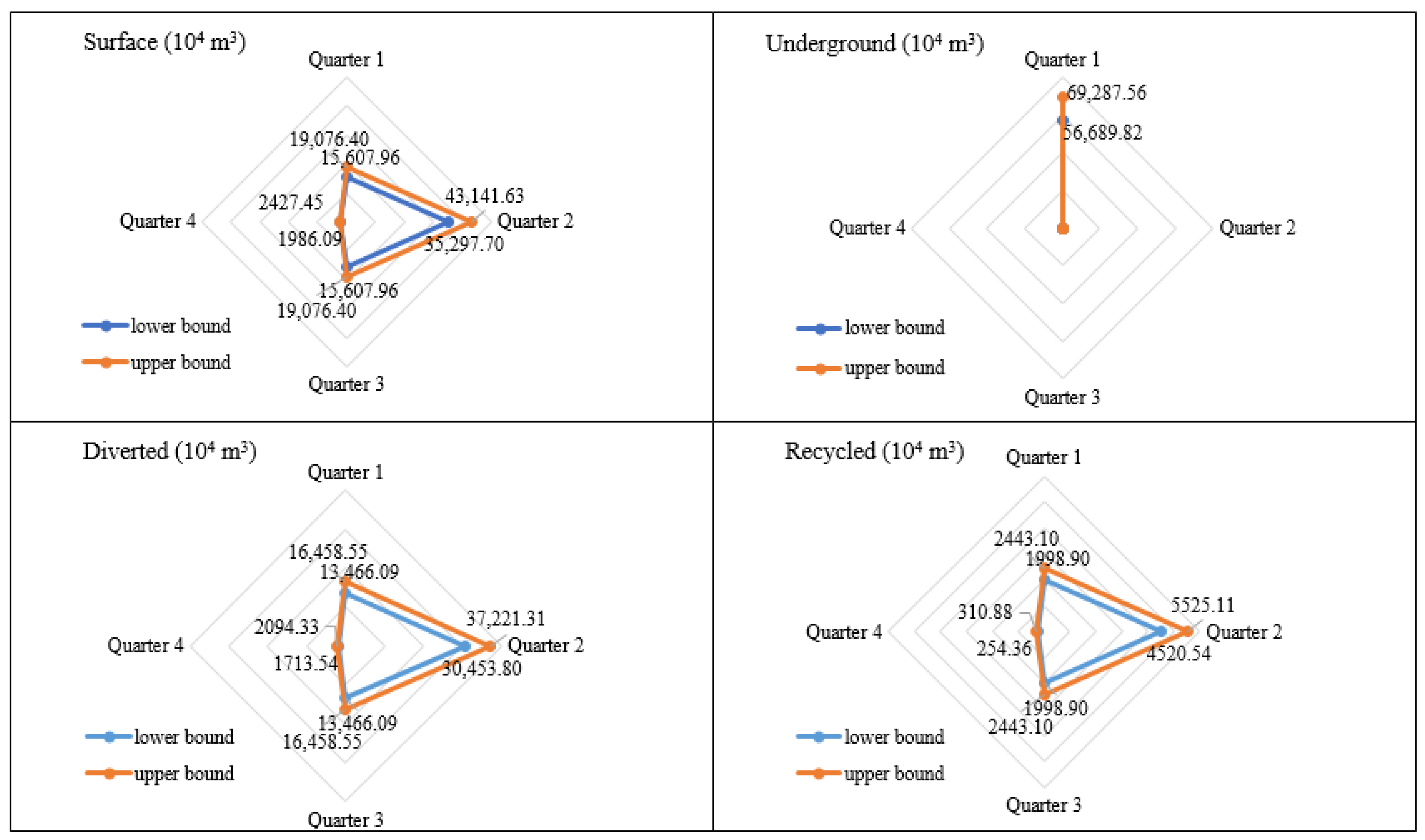
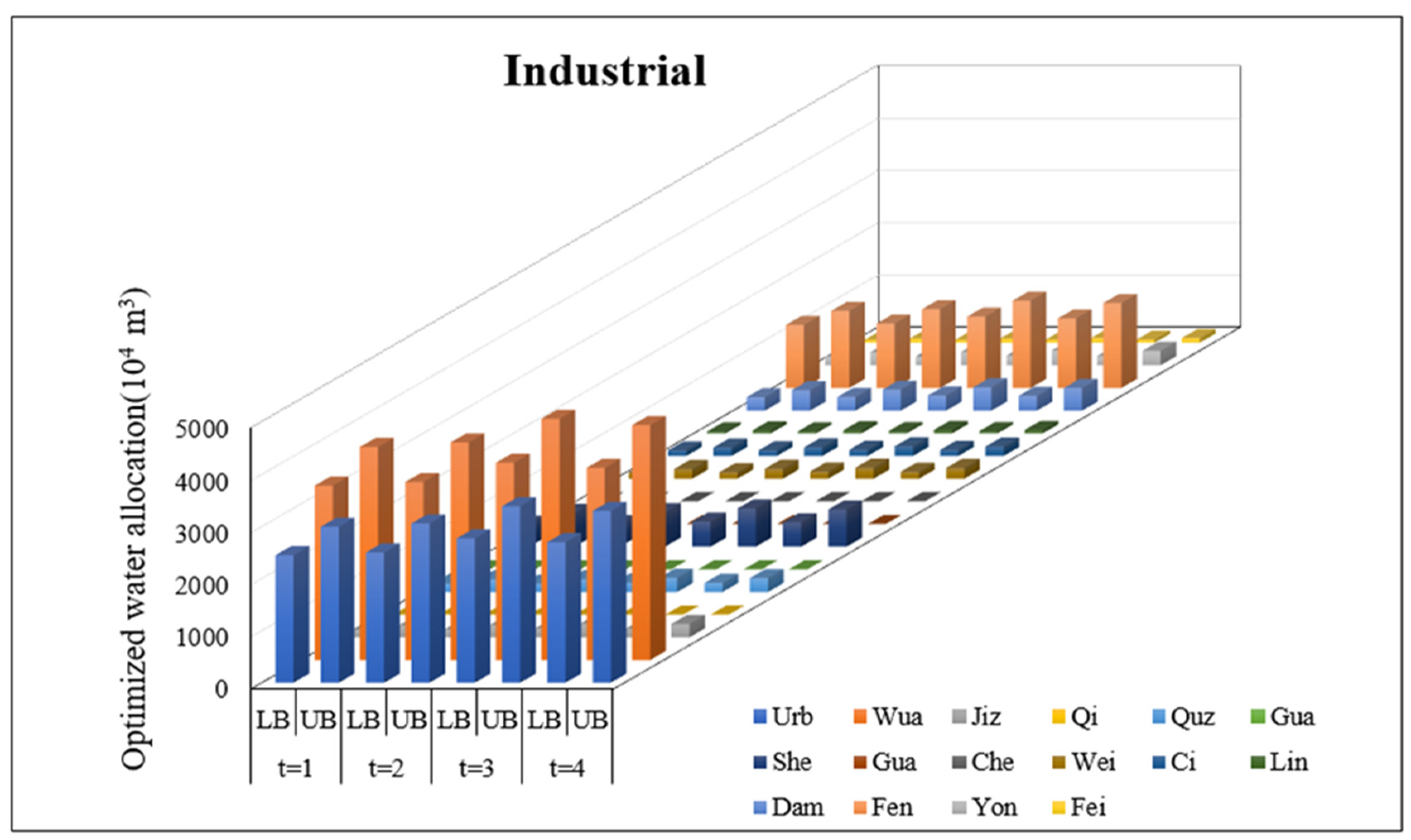
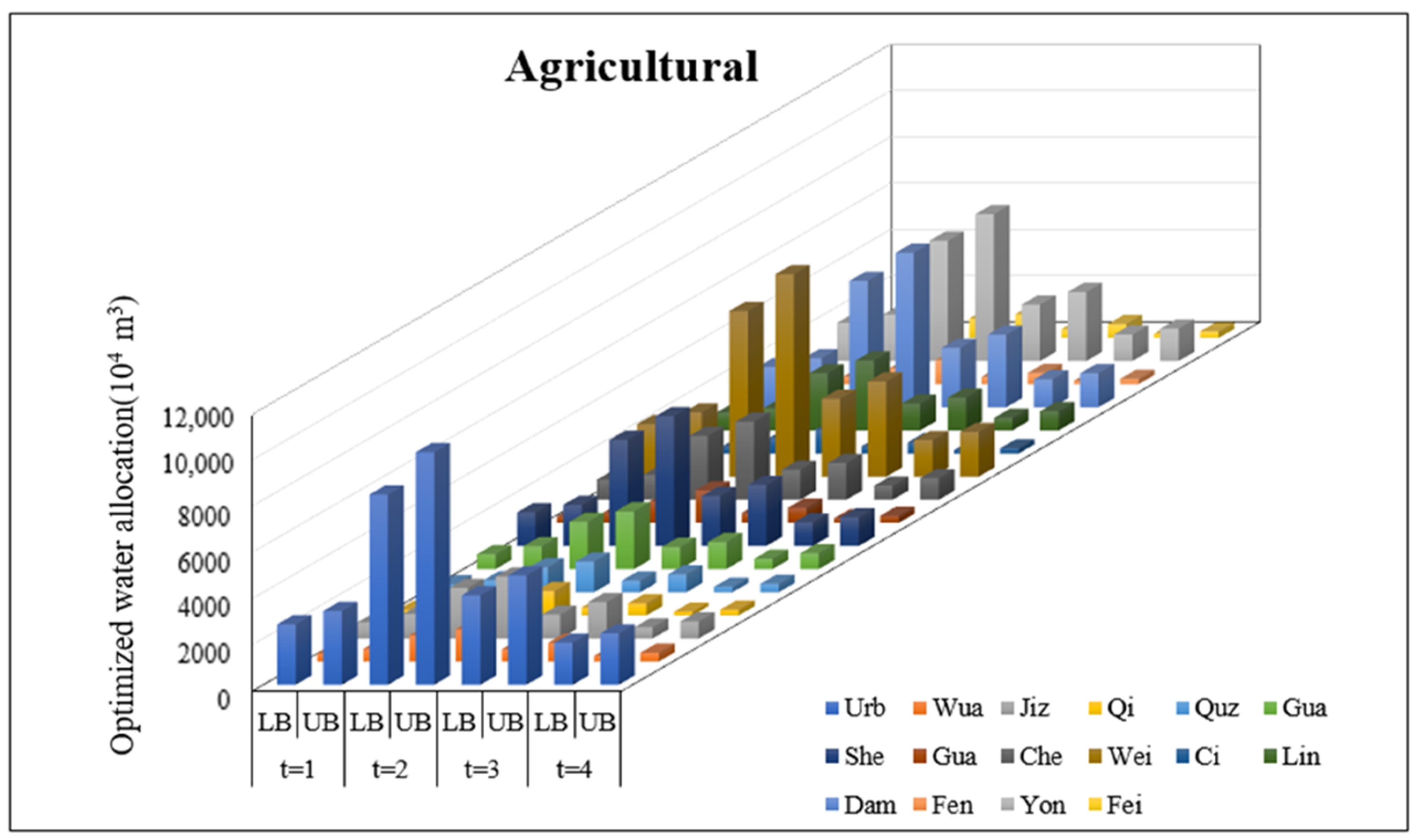
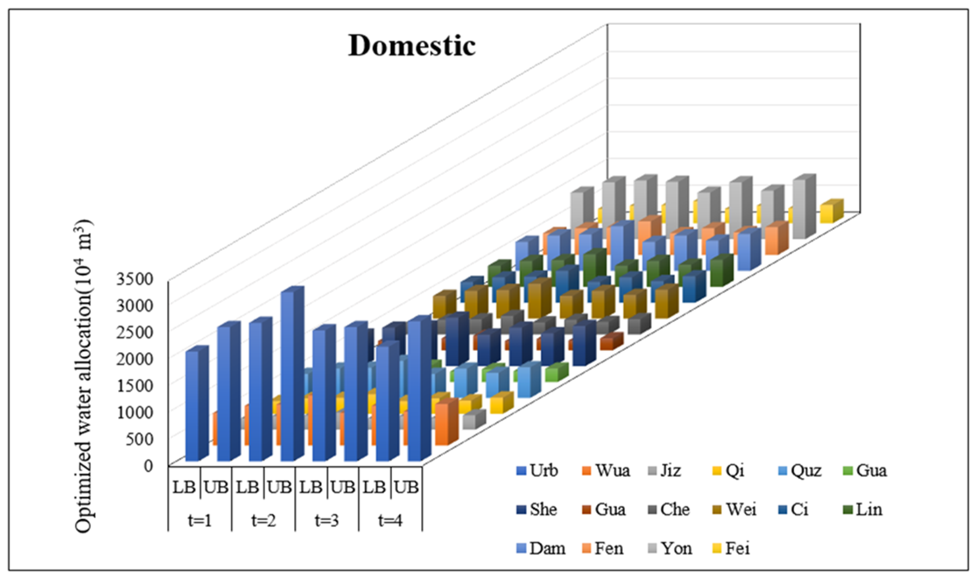
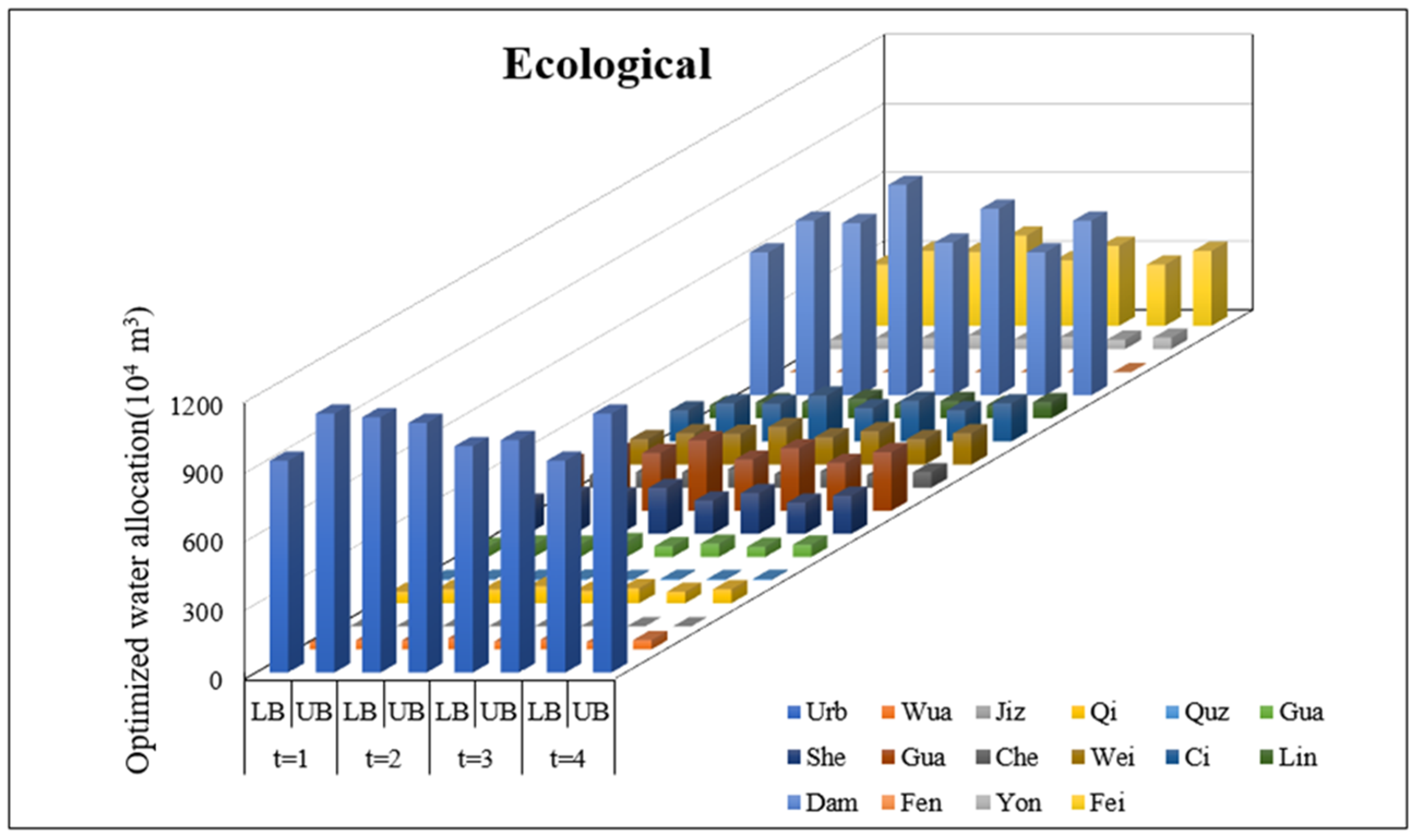
4.1. Results Analysis

In this study, the FIDP model suitable for Handan’s water management was established to obtain the objective function values and water resources allocation schemes, which can be seen in

Table 3. Solutions of objective functions (FIDP).

${\mathit{\lambda }}^{+} = 0.993$			${\mathit{\lambda }}^{-} = 0.985$
Economic Benefit (108 yuan)	Satisfaction	COD Emission (108 kg)	Economic Benefits (108 yuan)	Satisfaction	COD Emission (108 kg)
2989.33	96.50%	1.23	2264.72	87.50%	1.65

. The ${\lambda }^{+}$, ${\lambda }^{-}$ represent the maximum subordinate degree and the minimum subordinate degree respectively. In detail, by solving the model, the value of ${\lambda }_{opt}^{+}$ is 0.993, the corresponding economic benefit is 2989.33 × 10⁸ yuan, the satisfaction of users is 96.50%, and the social benefit is 1.23 × 10⁸ kg. On the contrary, the value of ${\lambda }_{opt}^{-}$ is 0.985, whilst the corresponding economic benefits, satisfaction and social benefits are 2264.72 × 10⁸ yuan, 87.50% and 1.65 × 10⁸ kg, respectively.

Table 4. Water allocations of different users in each region in the planning year (10⁴ m³).

Districts	Agricultural	Industrial	Domestic	Ecological
Urban	[16,518.74, 20,189.58]	[10,424.35, 12,740.87]	[9218.52, 10,784.89]	[3959.13, 4373.08]
Wuan	[2287.87, 3147.22]	[14,254.37, 17,422.01]	[2614.94, 3196.04]	[143.24, 175.07]
Jize	[4396.03, 6047.23]	[652.51, 996.90]	[901.13, 1101.38]	[0.00, 0.00]
Qiu	[1467.29, 2171.44]	[9.54, 14.58]	[1016.76, 1242.71]	[214.86, 262.60]
Quzhou	[2170.51, 2985.78]	[680.95, 1040.35]	[1926.37, 2354.45]	[19.10, 23.34]
Guantao	[4101.98, 5349.44]	[9.48, 13.05]	[845.26, 1033.10]	[190.99, 233.43]
She	[9225.72, 11,275.88]	[1809.88, 2765.09]	[2527.09, 3088.67]	[582.51, 711.95]
Guangping	[1847.23, 2822.16]	[0.00, 0.00]	[756.41, 924.50]	[895.73, 1094.78]
Chengan	[5545.87, 6964.69]	[23.25, 35.52]	[959.24, 1172.41]	[236.83, 289.45]
Wei	[14,383.22, 17,579.50]	[523.75, 800.17]	[1814.25, 2217.42]	[477.47, 583.57]
Ci	[1373.98, 2099.13]	[459.95, 702.70]	[1657.36, 2025.66]	[582.51, 711.95]
Linzhang	[4960.37, 6229.40]	[167.19, 255.43]	[1695.70, 2072.52]	[248.28, 303.46]
Daming	[10,977.77, 13,417.27]	[1103.89, 1686.50]	[2329.12, 2846.70]	[2669.02, 3262.14]
Fengfeng	[1371.38, 2095.17]	[5158.94, 6305.38]	[1755.10, 2145.12]	[0.00, 0.00]
Yongnian	[10,440.94, 12,761.14]	[706.91, 1080.00]	[3734.94, 4297.48]	[173.80, 212.42]
Feixiang	[1685.95, 2319.21]	[226.06, 345.37]	[1155.15, 1411.84]	[1145.92, 1400.56]

shows the total amount of water allocated to different users in different regions of Handan City in the planning year, while

Table 5. Water allocations of different water sources in each region in the planning year (10⁴ m³).

Districts	Surface Water	Groundwater	Diverted Water	Recycled Water
Urban	[7535.90, 21,990.98]	[6028.35, 26,097.44]	[0.00, 26,556.50]	[0.00, 0.00]
Wuan	[9076.72, 15,847.51]	[3943.55, 7350.32]	[0.00, 6246.64]	[33.52, 742.51]
Jize	[0.00, 3912.47]	[652.56, 996.90]	[1384.64, 6047.23]	[0.00, 1101.38]
Qiu	[14.58, 730.71]	[364.03, 852.45]	[1021.3, 2434.04]	[103.99, 878.69]
Quzhou	[306.46, 1086.30]	[1341.67, 2403.00]	[1068.88, 3009.12]	[238.76, 1746.66]
Guantao	[6.60, 3056.51]	[6.44, 1146.23]	[850.03, 5582.87]	[94.95, 1033.10]
She	[3913.91, 12,987.32]	[1950.42, 4550.79]	[0.00, 7365.07]	[303.47, 915.80]
Guangping	[0.00, 1352.17]	[0.00, 1320.49]	[534.83, 3916.94]	[291.86, 924.50]
Chengan	[27.17, 2761.84]	[351.78, 3361.19]	[525.30, 7254.14]	[116.86, 828.97]
Wei	[1968.76, 8824.34]	[399.29, 3747.87]	[1623.22, 18,163.07]	[649.55, 3003.27]
Ci	[894.02, 2402.74]	[537.57, 1705.73]	[1474.05, 2599.13]	[0.00, 0.00]
Linzhang	[1157.12, 3693.06]	[1170.83, 1810.47]	[1408.51, 6532.85]	[0.00, 159.50]
Daming	[9860.84, 15,954.89]	[1646.85, 3072.37]	[0.00, 5572.11]	[0.00, 2185.35]
Fengfeng	[5309.80, 5726.69]	[963.06, 4818.98]	[0.00, 1329.62]	[0.00, 682.95]
Yongnian	[4577.21, 6491.13]	[800.28, 5482]	[1263.73, 12,973.57]	[0.00, 1819.72]
Feixiang	[0.00, 753.86]	[675.35, 2026.42]	[875.11, 3719.78]	[328.00, 1311.54]

shows the total amount of water allocated from different water sources to different regions. It can be seen that the total amount of allocated water in Handan City in 2030 will be [175,412.60, 219,210.86] × 10⁴ m³, and the total water shortage will reach [34,051.91, 36,800.32] × 10⁴ m³ according to the water demand forecasting results. As the minimum water demand in the planning year will reach [167,571.50, 204,809.62] × 10⁴ m³, which is less than the allocated water, the water allocation in the planning year can meet its minimum guaranteed water demand on the whole.

In 2030, the agricultural water consumption in Handan City will account for [52.90, 53.60] % of the total water distribution with the detailed allocation being [92,754.97, 117,454.65] × 10⁴ m³. Since the agricultural water demand is affected by the season and climate, the water demand also changes at different stages of the planning year. In detail, the second stage is the main growth period of crops, and the agricultural water demand in this stage also increases correspondingly, accounting for [48.80, 49.80] % of the annual water demand. On the contrary, the amount of water distribution in the fourth stage accounts for the least proportion, which is only [11.10, 11.50] % of the total agricultural water distribution. The difference between these two stages is [35,988.55, 43,789.37] × 10⁴ m³. The calculation results show that the satisfaction of the agricultural is [80.00, 82.90] % in 2030, and it reaches 80% in each stage, meeting its minimum water demand. Supported by the soil characteristics of each region, the leading agricultural industries in Urban, Weixian, Daming, and Yongnian have been developing rapidly, and the agricultural water consumption in these four regions would account for [54.40, 56.40] % of the total agricultural water consumption in the city. The agricultural water distribution in the planning year is shown in Figure 4.

By solving the model, the industrial water distribution of Handan City in 2030 will be [36,210.94, 46,203.93] × 10⁴ m³, accounting for [20.60, 21.10] % of the total water distribution. The satisfaction of industrial water consumption is [80.00, 83.50] % in the whole year, and such satisfaction is higher than 80.00% in each stage, meeting its minimum water demand. According to the solution results as shown in Figure 5, the third stage has the largest industrial water distribution, which is [9631.84, 12,290.27] × 10⁴ m³, whereas the water distribution in the first stage is least with the allocation amount of [8509.83, 10,859.91] × 10⁴ m³, and the difference between the two stages is [1122.11, 1432.34] × 10⁴ m³. Among them, Urban, Wu’an and Fengfeng are the major industrial water users, making a contribution of [78.90, 82.40] % for the whole city’s industrial water consumption.

In 2030, the domestic water distribution in Handan City will be [34,907.31, 41,915.24] × 10⁴ m³, accounting for [19.10, 19.90] % of the total water distribution. The satisfaction of domestic water use in the whole year is [93.40, 95.10] %, and it is higher than 92.00% in each stage indicating a high degree for guaranteed domestic water. With the change of temperature, the domestic water consumption at different stages also changes slightly to some extent. Specifically, the proportion of domestic water in the four stages of the planning year is [23.01, 23.44] %, [28.80, 29.00] %, [23.40, 24.10] % and [24.00, 24.40] % respectively. Obviously, the second stage consumes the most domestic water, whereas the first stage consumes the least proportion. During the planning year, the population in Urban and Yongnian will reach 3.40 × 10⁶, and the water allocated to these two areas will be [12,953.41, 15,082.32] × 10⁴ m³ correspondingly, accounting for [36.00, 37.10] % of the domestic water distribution to the whole city. The annual domestic water distribution in the planning year is shown in Figure 6.

To a certain extent, the development degree of ecological environment reflects the sustainability level of the region. In 2030, the ecological water distribution in Handan will be [11,539.41, 13,638.02] × 10⁴ m³, with a contribution of [6.20, 6.60] % for the total water distribution. The satisfaction of ecological water use is [96.70, 100.00] % in the whole year with the satisfaction degree over 93.00% in each stage, which reflects the priority in ecological development. It can be seen from Figure 7 that the distribution of ecological water reaches the annual maximum amount of [3254.21, 3704.50] × 10⁴ m³ in the second stage, which is [404.34, 554.02] × 10⁴ m³ more than the least water distribution in the first stage. The ecological water consumption in the third and fourth stage is [2884.81, 3333.10] × 10⁴ m³ and [2700.24, 3300.23] × 10⁴ m³ respectively, accounting for [24.40, 25.00] % and [23.40, 24.20] % of the ecological water consumption in the whole year. Among them, the ecological water consumption in the urban area and Daming county is relatively huge, contribution [32.10, 34.30] % and [23.10, 23.90] % to the total ecological water consumption respectively. This indicates that these two regions pay close attention to ecological environment construction.

Based on the analysis above, it can be known that FIDP model can provide global optimal solutions for the planned annual water distribution scheme, as well as specific water distribution schemes at different stages of the year under dynamics and uncertainties. In the planning year, the second stage has the largest water distribution of [68,246.70, 84,190.91] × 10⁴ m³, while the fourth stage has the smallest water distribution of [30,648.40, 39,012.42] × 10⁴ m³. The water distribution difference between the two stages is [37,598.12, 45,178.58] × 10⁴ m³, and the difference accounts for [20.60, 21.40] % of the annual water distribution.

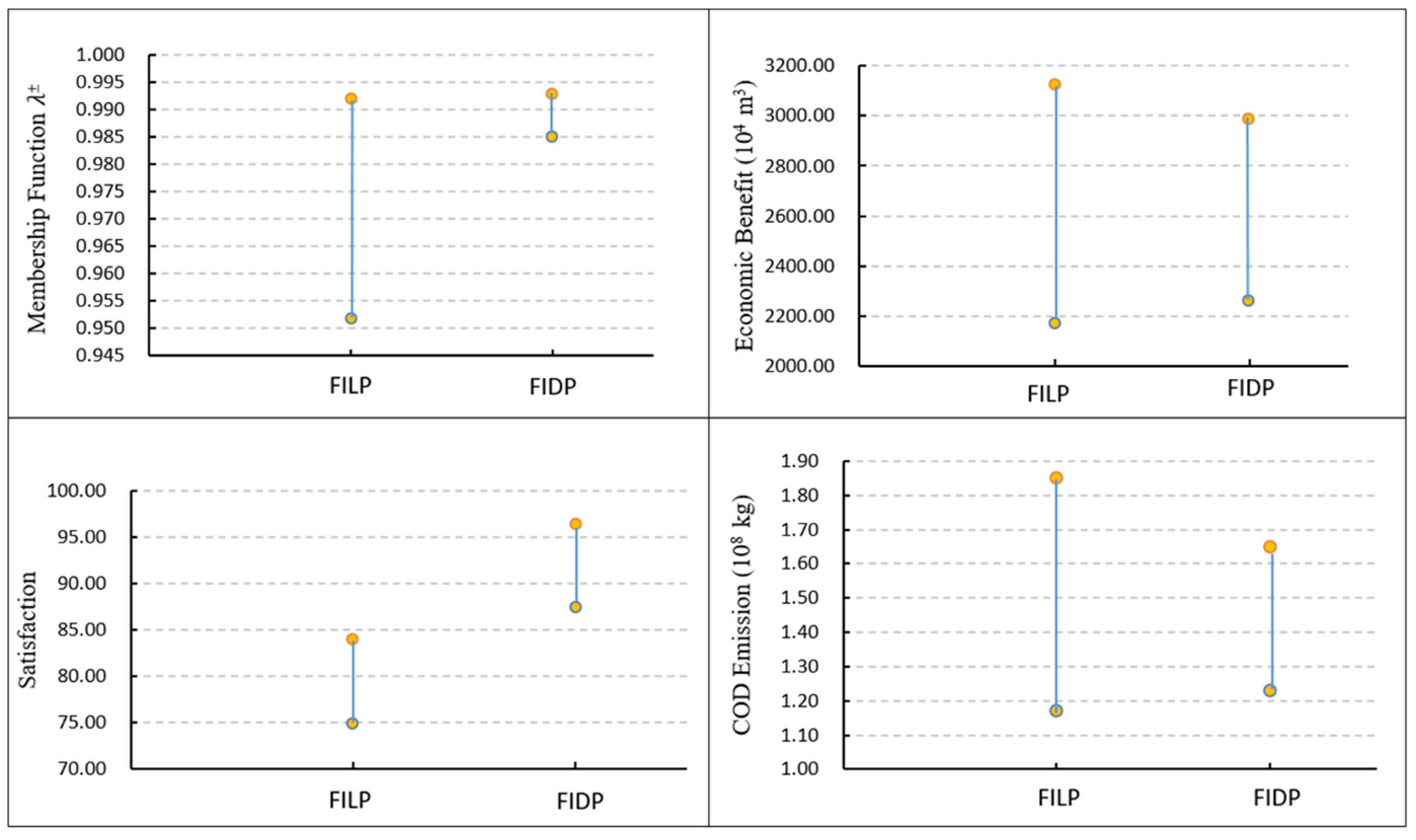
4.2. Model Comparison

In order to verify the effectiveness of the proposed FIDP model, the application of FILP model to the case study is provided for comparison, which is shown in Appendix A. The difference between FILP model and FIDP model is that it deletes dynamic programming and parameter t, but their objective functions, constraints, decision variables and solution methods remain the same. Because the FIDP model takes into account the dynamic factors in different stages of water resources system, the solution results cannot only conform to the case study, but also achieve global optimization under the local optimal conditions of each stage. However, the FILP model only aims at optimality over the whole planning year without considering the dynamic variability of regional water resources system, which would imply that the water use efficiency, water consumption, water demand, water supply and other factors in the FILP model cannot be adjusted correspondingly with the seasonal changes. Therefore, the FIDP model has better optimal solutions and stronger applicability than FILP. The detailed analysis is as follows.

Based on the FILP model, the membership function ${\lambda }^{\pm }$= [0.952, 0.992], $f_1^{\pm }$= [2171.42, 3124.16] × 10⁸ yuan, $f_2^{\pm }$= [75.00, 84.00] %, $f_3^{\pm }$= [1.17, 1.85] × 10⁸ kg, and the comparison result of two models is shown in Figure 8. It can be seen that, compared with the FILP model, the ranges of the solution results of the FIDP model are reduced in different degrees, making the results more specific and accurate. In detail, the ${\lambda }^{\pm }$ of the FIDP model is not only reduced in scope, but also presents increases in its overall value, with its upper bound and lower bounds increased by 0.10% and 3.30% respectively. For $f_1^{\pm }$ and $f_3^{\pm }$, not only the ranges of their value are reduced by 23.90% and 38.20%, but also their lower bounds are increased by 93.30 × 10⁸ yuan and 0.06 × 10⁸ kg respectively, which are more accurate. The value of $f_2^{\pm }$ in FIDP model is improved by 12.50%, which will alleviate the conflicts between local government and users, and among different users more effectively. Consequently, it can be concluded that FIDP model proposed in this paper performs better and is more suitable for the optimization of water resources allocation in this area.

The water distribution scheme of FILP model is shown in

Table 6. Water allocation of different users in different regions in the planning year (10⁴ m³).

	Agricultural	Industrial	Domestic	Ecological
Urban	[16,518.74, 20,189.58]	[10,424.35, 12,740.87]	[8824.00, 10,784.89]	[3167.30, 3871.15]
Wuan	[2287.87, 2796.29]	[14,254.37, 17,422.01]	[2091.95, 2556.83]	[143.23, 175.07]
Jize	[4396.03, 5372.93]	[652.51, 797.52]	[720.90, 881.11]	[0.00, 0.00]
Qiu	[1467.29, 1793.35]	[11.92, 14.58]	[813.41, 994.17]	[171.89, 262.60]
Quzhou	[2170.51, 2652.85]	[680.95, 832.28]	[1541.09, 1883.56]	[19.10, 23.34]
Guantao	[4101.98, 5013.54]	[10.67, 13.05]	[676.21, 826.48]	[152.79, 233.43]
She	[9225.72, 11,275.88]	[1809.88, 2212.07]	[2021.67, 2470.93]	[466.01, 569.56]
Guangping	[1847.23, 2257.73]	[0.00, 0.00]	[605.12, 739.60]	[716.58, 875.82]
Chengan	[5545.87, 6778.29]	[29.06, 35.52]	[767.39, 937.93]	[189.46, 289.45]
Wei	[14,383.22, 17,579.50]	[523.75, 640.14]	[1451.40, 1773.94]	[381.97, 484.41]
Ci	[1373.98, 1679.30]	[459.95, 562.16]	[1325.89, 1620.53]	[466.01, 569.56]
Linzhang	[4960.37, 6062.67]	[167.19, 255.43]	[1356.56, 1658.02]	[198.63, 303.46]
Daming	[10,977.77, 13,417.27]	[1103.89, 1349.20]	[1863.29, 2277.36]	[2135.22, 2609.71]
Fengfeng	[1371.38, 1676.14]	[5158.94, 6305.38]	[1404.08, 1716.10]	[0.00, 0.00]
Yongnian	[10,440.94, 12,761.14]	[706.91, 864]	[2987.95, 3651.94]	[167.60, 212.42]
Feixiang	[1685.95, 2060.61]	[226.06, 345.37]	[924.12, 1129.48]	[916.73, 1120.45]

, and the water shortage rate of the two models is compared in Figure 9. As presented in Table 6, the total water distribution of the FILP model is [167,643.11, 205,259.94] × 10⁴ m³, which is reduced by [7769.43, 13,951.80] × 10⁴ m³ compared with the FIDP model. As the water distribution decreases, the corresponding water shortage rate will be [19.70, 20.00] %, with an increase of [5.10, 9.10] % compared with [10.60, 14.90] % from the FIDP model. Compared with FILP, the water shortage rate from FIDP has declined in all regions, especially in Qiu, Quzhou, Guangping, Ci and Feixiang, with a decrease of [7.90, 16.70] %, [7.00, 15.00] %, [8.30, 20.00] %, [9.90, 20.00] %, and [9.80, 14.30] % respectively. Therefore, the model has good applicability to water resources allocation in water-scarce areas.

In summary, the FIDP model has the following advantages over the FILP model: (i) The obtained target value intervals are more specific and accurate. (ii) This model can improve the overall satisfaction of the water users and alleviate the water contradiction among them. (iii) The water shortage rate of FIDP model is lower than that of FILP, which effectively alleviates the contradiction between water supply and demand. (iv) Last but not least, FIDP model can get the allocation schemes of each stage in the planning year, and provide theoretical basis for water distribution decision-making in more detail way. Therefore, the model has a good performance in dealing with the dynamic changes of water resources system, and has advantages in optimizing the target value and reducing the water shortage rate.

5. Conclusions

This study combines fuzzy-interval linear programming and dynamic programming to establish a fuzzy-interval dynamic programming (FIDP) method. The system uncertainty is expressed in the form of interval numbers in the model establishment and results presentation. In order to solve the conflicts among users caused by uneven distribution of resources, the FIDP model incorporates the overall satisfaction of users into the objective function in order to reflect fairness in the solution results. As for the dynamic variability, the FIDP model introduces dynamic programming to obtain the specific allocation schemes at different stages of the planning year. Therefore, the model is able to handle the problem of uneven resources allocation under uncertainty and dynamics.

In this paper, the water resources allocation under uncertainty and dynamics in Handan City is studied to verify the feasibility of the model. The solutions cannot only get the optimized target value in this area, but also get the specific water allocations and water shortages for each water user at different stages in the form of intervals, so that the government and users can adjust their strategies to deal with the crisis in time. In addition to the economic and environmental goals, the obtained solution also provides the satisfaction of water users by introducing a weight coefficient, which effectively alleviates the contradictions among users. Through model comparison, the FIDP is proved to be superior to FILP model in this area. Consequently, the developed FIDP model would be more rational and applicable for regional water allocation under uncertainty and dynamics, which is of great help to the sustainable development of the region.

References

1. UN Water. The United Nations World Water Development Report 2020: Water and Climate Change; UNESCO: Paris, France, 2020. [Google Scholar]
2. Kang, A.; Li, J.; Lei, X.; Ye, M. Optimal allocation of water resources considering water quality and the absorbing pollution capacity of water. Water Resour. 2020, 47, 336–347. [Google Scholar] [CrossRef]
3. Xiao, Y.; Fang, L.; Hipel, K.W. Conservation-targeted hydrologic-economic models for water demand management. J. Environ. Inform. 2019, 37, 49–61. [Google Scholar] [CrossRef]
4. Wang, L.; Huang, Y.; Zhao, Y.; Li, H.; He, F.; Zhai, J.; Zhu, Y.; Wang, Q.; Jiang, S. Research on optimal water allocation based on water rights trade under the principle of water demand management: A case study in Bayannur City, China. Water 2018, 10, 863. [Google Scholar] [CrossRef] [Green Version]
5. Sun, J.; Li, Y.P.; Suo, C.; Liu, J. Development of an uncertain water-food-energy nexus model for pursuing sustainable agricultural and electric productions. Agr. Water Manag. 2020, 241, 106–384. [Google Scholar] [CrossRef]
6. Zhang, Y.F.; Li, Y.P.; Sun, J.; Huang, G.H. Optimizing water resources allocation and soil salinity control for supporting agricultural and environmental sustainable development in Central Asia. Sci. Total Environ. 2019, 704, 135281. [Google Scholar] [CrossRef] [PubMed]
7. Sun, Y.G.; Gu, S.H.; He, J.K. Game Analysis for Conflicts in Water Resource Allocation. Syst. Eng.-Theory Pract. 2022, 1, 16–25. [Google Scholar]
8. Ren, C.H.; Guo, P.; Li, M.; Gu, J.J. Optimization of industrial structure considering the uncertainty of water resources. Water Resour. Manag. 2013, 27, 3885–3989. [Google Scholar] [CrossRef]
9. Yang, G.Q.; Li, M.; Guo, P. Monte Carlo-Based Agricultural Water Management under Uncertainty: A Case Study of Shijin Irrigation District, China. J. Environ. Inform. 2020. [Google Scholar] [CrossRef]
10. Sun, J.; Li, Y.; Suo, C.; Liu, Y. Impacts of irrigation efficiency on agricultural water-land nexus system management under multiple uncertainties—A case study in Amu Darya River basin, Central Asia. Agr. Water Manag. 2019, 216, 76–88. [Google Scholar] [CrossRef]
11. Fan, Y.; Huang, W.; Li, Y.; Huang, G.; Huang, K. A coupled ensemble filtering and probabilistic collocation approach for uncertainty quantification of hydrological models. J. Hydrol. 2015, 530, 255–272. [Google Scholar] [CrossRef] [Green Version]
12. Bravo, M.; Gonzalez, I. Applying stochastic goal programming: A case study on water use planning. Eur. J. Oper. Res. 2009, 196, 1123–1129. [Google Scholar] [CrossRef]
13. Kumar, S.S.; Prasad, Y.S. Modeling and optimization of multi object non-linear programming problem in intuitionistic fuzzy environment. Appl. Math. Model. 2015, 39, 4617–4629. [Google Scholar]
14. Fan, Y.R.; Huang, G.H.; Li, Y.P. Robust interval linear programming for environmental decision making under uncertainty. Eng. Optimi. 2012, 44, 1321–1336. [Google Scholar] [CrossRef]
15. Zou, R.; Liu, Y.; Liu, L.; Guo, H. REILP Approach for uncertainty-based decision making in civil engineering. J. Comput. Civ. Eng. 2010, 24, 357–364. [Google Scholar] [CrossRef]
16. Zeng, X.; Chen, C.; Sheng, Y.; An, C.; Kong, X.; Zhao, S.; Huang, G. Planning Water Resources in an agroforest ecosystem for improvement of regional ecological function under uncertainties. Water 2018, 10, 415. [Google Scholar] [CrossRef] [Green Version]
17. Zhang, J.; Huang, G.H.; Liu, Y.; Kai, A.N. Dispatch model for combined water supply of multiple sources under the conditions of uncertainty. J. Hydraul. Eng. 2009, 40, 160–165. [Google Scholar]
18. Huang, G.H.; Loucks, D.P. An inexact two-stage stochastic programming model for water resources management under uncertaint. Civ. Eng. Environ. Syst. 2000, 17, 95–118. [Google Scholar] [CrossRef]
19. Zhou, F.; Huang, G.; Chen, G.-X.; Guo, H.-C. Enhanced-interval linear programming. Eur. J. Oper. Res. 2009, 199, 323–333. [Google Scholar] [CrossRef]
20. Liu, Y.; Guo, H.; Zhou, F.; Qin, X.; Huang, K.; Yu, Y. Inexact chance-constrained linear programming model for optimal water pollution management at the watershed scale. J. Water Res. Plan. Manag. 2008, 134, 347–356. [Google Scholar] [CrossRef]
21. Gu, J.J.; Huang, G.H.; Guo, P.; Shen, N. Interval multistage joint-probabilistic integer programming approach for water resources allocation and management. J. Environ. Inform. 2013, 128, 615–624. [Google Scholar] [CrossRef] [PubMed]
22. Guo, P.; Chen, X.H.; Li, M.; Li, J.B. Fuzzy chance-constrained linear fractional programming approach for optimal water allocation. Stoch. Environ. Res. Risk Assess. 2014, 28, 1601–1612. [Google Scholar] [CrossRef]
23. Wang, H.; Zhang, C.; Ping, G. An interval quadratic fuzzy dependent-chance programming model for optimal irrigation water allocation under uncertainty. Water 2018, 10, 684. [Google Scholar] [CrossRef] [Green Version]
24. Han, Y.; Huang, Y.-F.; Wang, G.-Q.; Maqsood, I. A multi-objective linear programming model with interval parameters for water resources allocation in Dalian city. Water Resour. Manag. 2011, 25, 449–463. [Google Scholar] [CrossRef]
25. Li, M.; Guo, P. A Multi-objective optimal allocation model for irrigation water resources under multiple uncertainties. Appl. Math. Model. 2014, 38, 4897–4911. [Google Scholar] [CrossRef]
26. Suo, M.Q.; Wu, P.F.; Zhou, B. An Integrated Method for Interval Multi-Objective Planning of a Water Resource System in the Eastern Part of Handan. Water 2017, 9, 528. [Google Scholar] [CrossRef] [Green Version]
27. Li, J.; Qiao, Y.; Lei, X.; Kang, A.; Wang, M.; Liao, W.; Wang, H.; Ma, Y. A two-stage water allocation strategy for developing regional economic-environment sustainability. J. Environ. Inform. 2019, 244, 189–198. [Google Scholar] [CrossRef] [PubMed]
28. Burt, O.R. On optimization methods for branching multistage water resource systems. Water Resour. Res. 2010, 6, 345–346. [Google Scholar] [CrossRef]
29. Liu, H.Q.; Zhao, Y.; Li, H.H. Optimal water resources allocation based on interval two-stage stochastic programming in Beijing. South-North Water Transf. Water Sci. Technol. 2020, 18, 34–41. [Google Scholar]
30. Trzaskalik, T. Multi-objective dynamic programming in bipolar multistage method. Ann. Oper. Res. 2021, 4, 1–21. [Google Scholar]
31. Agliardi, R. Optimal hedging through limit orders. Stoch. Models 2016, 32, 593–605. [Google Scholar] [CrossRef]
32. Huang, K.C.; Lu, H. A Linear Programming-based Method for the Network Revenue Management Problem of Air Cargo. Transp. Res. Procedia 2015, 7, 459–473. [Google Scholar] [CrossRef] [Green Version]
33. Elvan, G. Fertilizer application management under uncertainty using approximate dynamic programming. Comput. Ind. Eng. 2021, 161, 107624. [Google Scholar]
34. Liu, H.; Wang, Y.; Liu, S.; Liu, Q.; Xie, Y.; Ma, X. Research on multi-objective optimal scheduling strategy of photovoltaic and energy storage based on dynamic programming. IOP Conf. Ser. Earth Environ. Sci. 2021, 781, 42011. [Google Scholar] [CrossRef]
35. Peng, J.; Yuan, X.; Qi, L.; Li, Q. A study of multi-objective dynamic water resources allocation modeling of Huai River. Water Sci. Tech-Water Sup. 2015, 15, 817. [Google Scholar] [CrossRef]
36. Feng, J.H. Optimal allocation of regional water resources based on multi-objective dynamic equilibrium strategy. Appl. Math. Model. 2021, 90, 1183–1203. [Google Scholar] [CrossRef]
37. Ramírez, R.M.; Juárez, M.L.A.; Mora, R.D.; Morales, L.D.P.; Mariles, Ó.A.F.; Reséndiz, A.M.; Elizondo, E.C.; Paredes, R.B.C. Operation Policies through Dynamic Programming and Genetic Algorithms, for a Reservoir with Irrigation and Water Supply Uses. Water Resour. Manag. 2021, 35, 1573–1586. [Google Scholar] [CrossRef]
38. Fan, Y.R.; Huang, G.H.; Veawab, A. A generalized fuzzy linear programming approach for environmental management problem under uncertainty. J. Air Waste Manag. Assoc. 2012, 62, 72–86. [Google Scholar] [CrossRef] [PubMed] [Green Version]
39. Fan, Y.R.; Huang, G.H.; Huang, K.; Baetz, B.W. Planning water resources allocation under multiple uncertainties through a generalized fuzzy two-stage stochastic programming method. IEEE Trans. Fuzzy Syst. 2015, 23, 1488–1504. [Google Scholar] [CrossRef]
40. Nie, S.; Huang, C.Z.; Huang, W.W.; Liu, J. A Non-Deterministic Integrated Optimization Model with Risk Measure for Identifying Water Resources Management Strategy. J. Environ. Inform. 2021, 38, 41–55. [Google Scholar] [CrossRef]
41. Deng, Y.; Xu, Z.; Zhou, L.; Liu, H.; Huang, A. Study on adaptive chord allocation algorithm based on dynamic programming. J. Fudan Univ. (Nat. Sci.) 2019, 58, 393–400. [Google Scholar]
42. Bellman, R.E.; Kalaba, R.E.; Teichmann, T. Dynamic programing. Phys. Today 1966, 19, 99–105. [Google Scholar]
43. Ye, X. Practical Operations Research; China Renmin University Press: Beijing, China, 2013. [Google Scholar]
44. Guo, Y.X. Operations Research; South China University of Technology Press: Guangzhou, China, 2012. [Google Scholar]
45. Wang, X.; Huang, G.H. Violation analysis on two-step method for interval linear programming. Inform. Sci. 2014, 281, 85–96. [Google Scholar] [CrossRef]
46. Handan Water Conservancy Bureau. Handan Water Resources Bulletin; Handan City General Management Office: Handan, China, 2019. [Google Scholar]
47. Handan Bureau of Statistics. Handan Statistical Yearbook; China Statistics Press: Beijing, China, 2017. [Google Scholar]
48. Wang, M.J. Multiobjective Planning of Water Resources in Wuhu City; Hefei University of Technology: Hefei, China, 2018. [Google Scholar]
49. Wang, Y.J. Study on Optimal Allocation of Water Resources in Sixian County based on Multi Objective Programming; Hebei University of Engineering: Handan, China, 2020. [Google Scholar]
50. Liu, M.Y. Research on Security Evaluation and Optimal Allocation of Water Resources in Haixing County; Hebei University of Engineering: Handan, China, 2019. [Google Scholar]
51. Li, S.; Liu, B. Application of improved artificial fish swarm algorithm in optimal allocation water resources in Handan. Water Resour. Power 2016, 34, 10–14. [Google Scholar]
52. Liu, Y.L.; Cao, W.J.; Li, F. Application of metabolic GM(1, 1) power model in predicting the incidence of viral hepatitis. Chin. J. Health Stat. 2019, 36, 854–856. [Google Scholar]
Figure 1. Location of Handan city.
Sustainability 14 01096 g001
Figure 2. Framework of the fuzzy-interval dynamic programming (FIDP) model.
Sustainability 14 01096 g002
Figure 3. The amount of different water sources in the planning year (104 m3).
Sustainability 14 01096 g003
Figure 4. Water allocations for agricultural use in the planning year.
Sustainability 14 01096 g004
Figure 5. Water allocations for industrial use in the planning year.
Sustainability 14 01096 g005
Figure 6. Water allocations for domestic use in the planning year.
Sustainability 14 01096 g006
Figure 7. Water allocations for ecological use in the planning year.
Sustainability 14 01096 g007
Figure 8. Comparison of the objective functions between FILP and FIDP.
Sustainability 14 01096 g008
Figure 9. Comparison of water shortage rates between FILP and FIDP.
Sustainability 14 01096 g009