MODFLOW and HYDRUS Modeling of Groundwater Supply Prospect Assessment for Distant Pastures in the Aksu River Middle Reaches

Abstract

As in many regions across the world, southeastern Kazakhstan is subjected to ongoing water-resource depletion. The livestock sector is already a major natural water resource consumer, with groundwater use becoming its water supply strategy. Remote pasture infrastructure development requires new water resources to allow pasture area circulation. The distant pastures in the middle reach of the Aksu River consist of three pastures, with a total area of 32,450 ha and a permissible number of 3245 livestock heads. The HYDRUS-1D water transport model and MODFLOW groundwater-flow model simulated complex water infrastructure prospect hydrogeological scenarios to allow the consumption of 302.4 m³ per day for livestock keeping on pasturelands. During pumping for livestock watering, projected production well drawdowns were quantitatively evaluated. The findings show that the projected pumping flow rate equals 288 m³/day during the water consumption season and 95 m³/day outside the water consumption season. While the production wells on pastures No. 2 and No. 3 can be considered reliable, on pasture No. 1, an additional production well is needed. To maintain the production wells’ drawdowns to less than 6 m, a projected pumping flow rate reduction to 216 m³/day and 70 m³/day, respectively, is required.

1. Introduction

One consequence of global climate change is that inland watersheds are drying out [1]. Southeastern Kazakhstan’s water-resource deficit is compounded by the large distances to natural water sources of good quality, which requires the use of groundwater from local aquifers to supply the local population and agriculture needs with good-quality drinking water. The livestock sector currently utilizes approximately 35% of all arable land and approximately 20% of the water, and these numbers are constantly on the rise [2]. To allow this gradual development needed for complying with food production demand, improving livestock water productivity is essential, as water scarcity becomes a limiting factor [3]. The Food and Agriculture Organization of the United Nations (FAO) integration of detailed data on feed use and livestock production with statistics and process-based crop-water model simulations enables a comprehensive assessment of water use and water productivity in the global livestock sector [4]. Water scarcity is related to surface and groundwater depletion and not to total water outflow from agricultural systems [5]. This problem is common in other regions, such as parts of the Canadian prairies, where low-quality agricultural runoff prevents surface water from being a dependable water source for livestock. In these areas, farmers need to drill water wells or pump water into stock tanks for their livestock [6].

The use of groundwater for distant pasture water supply system design and management involves geological, geochemical, hydrological, biological and engineering aspects. To develop an integrated solution to water supply design, a numerical computer modeling approach with groundwater regional recharge rate estimation is required [7]. The Kishi-Tobe settlement drinking water and artificial recharge pumping wells’ optimal location was forecasted in terms of both drawdown and groundwater resource provision balance by MODFLOW modeling [8]. An Integrated Water Flow Model (IWFM) enabled groundwater management planning under complex conflicting requirements [9].

A regional three-dimensional finite element groundwater-flow model of Brazil’s Guarani Aquifer System strategic water supply, which is transboundary to Argentina, Paraguay and Uruguay, was constructed to obtain a better understanding of prevailing flow dynamics and a more reliable groundwater recharge estimation [10]. Spatiotemporal groundwater recharge was studied in gauged and ungauged agro–urban watersheds in South Korea using the updated SWAT-MODFLOW model [11]. Groundwater Flow Finite Difference Modeling shows that artificial direct injection recharge into an aquifer prevents runoff evaporation and outflow from the watershed and increases aquifer recharge, as well as irrigation potential [12]. A stratified porous medium mathematical model of artificial groundwater recharge based on infiltration wells takes into account all the soil profile characteristics and enables better decision-making in pasture management [13]. Grazing rotation pasture growth stages in New Zealand were estimated based on crop coefficients and evapotranspiration, indicating that crop coefficient variations and pasture growth stages are irrigation scheduling dependent and that, once optimized, they may reduce drainage and overland flow without affecting pasture productivity [14].

Pasture husbandry in Kazakhstan involves the infrastructure development of remote pasture areas to allow pasture circulation. Under these conditions, the application of surface water infiltration based on artificial groundwater-recharge techniques can be an efficient way to provide remote pasture areas with water. Infiltration is a process by which water enters the soil, and it is one of the key fluxes in the hydrological cycle that affect the soil water balance [15,16,17]. The experimental studies carried out at the Karatal experimental site evaluated the infiltration and clogging processes and the silting in the mini pool’s infiltration profile [18,19]. Detailed assessments of cover deposits, upper aquifer layers and water-physical, hydrodynamic and filtration properties play a significant role in infiltration and colmatation processes [20].

Surface infiltration and groundwater level estimations in the Israeli Coastal Aquifer during desalinated seawater and managed groundwater recharge from an infiltration pond were attained by simple analytical models, and a numerical model was used for estimating groundwater recharge after the end of infiltration [21]. It was found that a calibrated numerical model with a one-dimensional representative sediment profile (HYDRUS-1D) can capture infiltration dynamics, including temporal infiltration rate reduction, drainage and groundwater recharge [22].

Understanding water and solute movement processes in unsaturated soil layers requires a mathematical description and numerical model development [22,23,24,25]. Water and solute movement models in an unsaturated soil layer are based on Richards’ equation for one-dimensional water movement under saturation variability [24,26], and root water up-take is calculated. The water retention curve can be described by the van Genuchten Equation [27]. In such models, the saturated soil hydraulic conductivity coefficient is a factor that varies with the soil’s hydraulic conductivity function.

The most popular numerical hydraulic function with whom methods for solving the nonlinear Richards’ equation is endowed is the van Genuchten-Mualem (no hysteresis) single porosity hydraulic model. Another well-known hydraulic function numerical method used to solve the nonlinear in the Richards’ equation is Gardner’s hydraulic functions using the Kirchhoff integral transformation approach [28,29]; nevertheless, since applying a combined MODFLOW and HYDRUS modeling, the van Genuchten-Mualem model is rather conventional [30]; it was applied in this study.

Water supply, well construction and maintenance require substantial financial resources, which might hinder pasture development and, in particular, deny distant pasture watering measures [23]. Within the Kazakh Agriculture Ministry’s “Agribusiness 2020” program, since 2013, a framework of solar- and wind energy-based irrigation from 4000 wells has been under development to sustain more than 8.0 million pastureland hectares, with costs amounting to approximately KZT 28 billion tenges (USD ~60 million).

The project’s master plan involved information from a geo-botanical survey of pastures and veterinary and sanitary facilities, including livestock and farm animal data, by several herds and flocks. The data integration enabled farm grazing potential assessment in distant pastures and grazing peculiarities on cultivated and arid pastures. The Aksu River middle reaches distant pastures bearing a total area of 32,450 ha of the Aksu district in the Almaty administrative region. The pasture fodder period is 200–220 days, and the fodder period total livestock watering demand is 63,318 m³, with pasturelands daily livestock maintaining a water consumption of 302.4 m³. The recommended permissible number of livestock on pasturelands is 3245 heads, whereas groundwater-based water supply restoration and development is needed for maintaining and extending this number.

In this manner, the study objectives were to assess the water supply required for pasture management and development and to supply needed groundwater prospects for the Aksu River middle reaches based on integrated MODFLOW and HYDRUS-1D model simulation.

2. Materials and Methods

2.1. Research Site Background and Geographical Framework

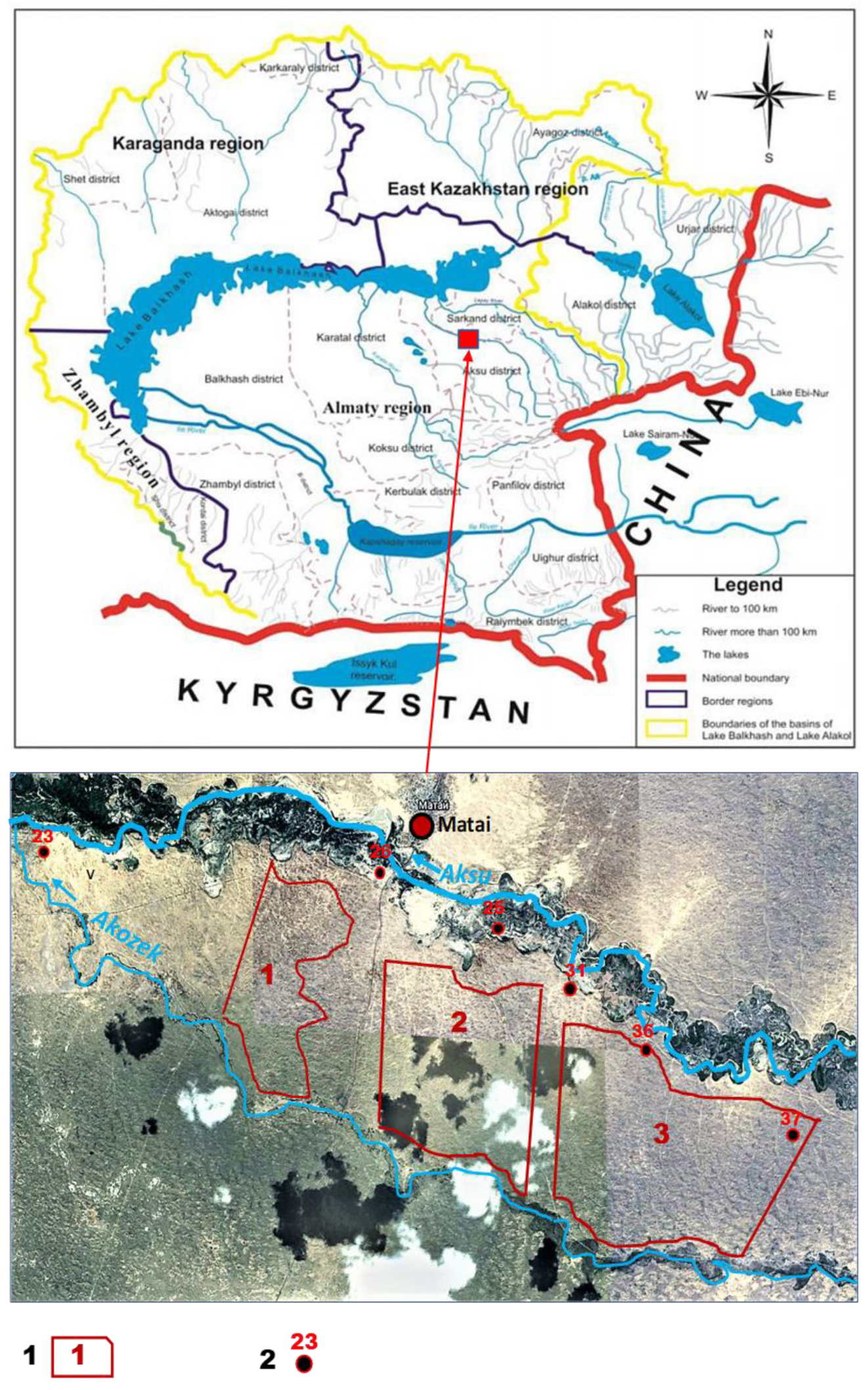
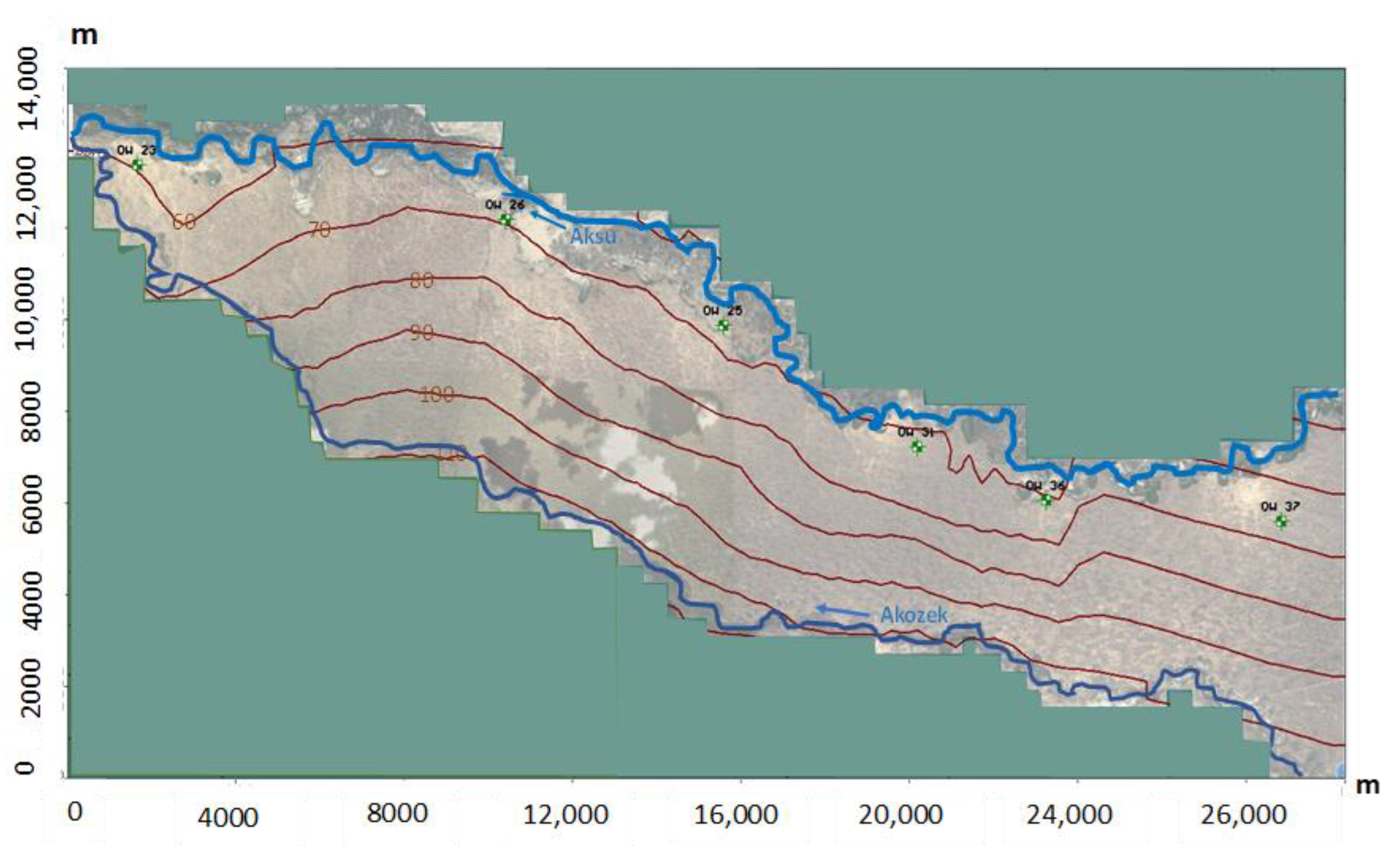
The Aksu research site is located in the northern part of the Aksu district on the Aksu River’s middle left bank. The Aksu River has the highest water volume in southeastern Kazakhstan until its outlet into Kukan Bay at Lake Balkhash’s eastern part (Figure 1). The Aksu riverbed is the research site’s northern boundary, and the southern and western boundaries are the Akozek River, which is an intermittent river with runoff running to its full extent during the rainy season and with nearly no overground flow during the dry season peak. The site’s eastern border is the Aksu-Akozek interfluve area, which has limited land with soil and vegetation suitable for distant pasture infrastructure restoration and development potential. The research site’s total area is approximately 470 km², of which 325 km² is allocated for pasture development.

The study area’s climate is extremely continental, characterized by cold winters, hot summers and short springs and autumn. During 2017–2019, the minimum average monthly air temperature was in January (−17.9 °C), and the maximum was in July (+26.9 °C). The period with a constant temperature above 10 °C varied from 183 to 193 days. The annual precipitation distribution pattern is of the highest amount (from 250 to 370 mm) during March, April, May and June; the peak flood season occurs in July/August, and during January, October, November and December, the precipitation amount is from 110 to 135 mm.

The main role of groundwater recharge is the creation of moisture reserves in the soil’s root layer during the winter when precipitation is mainly in the form of snow and hail. Due to the high evaporation values of the warm period, the precipitation practically does not infiltrate to form moisture reserves. The long-term averaged annual evaporation value from the open ground surface is 650 mm and from the Aksu River water surface is 1050 mm. The total Aksu River length is approximately 316 km, and its basin area is 4100 km². The Aksu River originates in the Dzungarsky Alatau Mountains and glacial moraine lakes. It flows in a steep gradient while in the mountains and takes on a flat character, with an average hydraulic slope of 0.0005%, until it ends in Balkhash Lake. The Aksu River has 132 tributaries with a total length of 213 km. The river recharge is mainly from glaciers and snowmelt, as well as from underground sources. The river flow is regulated by a reservoir system, and a small hydroelectric power station was built on the river near the Zhansugurov settlement for local needs. The river section in the study site has a width of 40–50 m and a gradient of 16.3 m. At the study site’s western border, the river’s bottom height above sea level is 411.6 m, and at the eastern border, it is 427.9 m. The depth of the river in this area varies from 0.9 to 1.5 m and from 0.6 to 1.15 m, respectively, depending on the annual rainfall [19].

The Aksu River average annual water flow rate in the research site is 25 m³/s (0.6 km³/year) at 25% probability, 15 m³/s (0.45 km³/year) at 50% and 8 m³/s (0.25 km³/year) at 75% probability. The averaged long-term flow rate is 18 m³/s, with a maximum equal to 28 m³/s and a minimum equal to 5 m³/s. Floods with a maximum flow rate of up to 45 m³/s occur in May, June and July and less in August. Water mineralization was performed with calcium bicarbonate at a concentration of 0.3–0.5 g/L.

The Aksu research site is in a flat alluvial plain, with distinct fluvial features: floodplain and low floodplain terraces; flat accumulative takyr-like plain; shallow sandy plain, and a plain with hilly ridge eolian relief. The soil type distribution is closely related to the climatic, geomorphological and hydrogeological conditions. Alluvial meadow soils have formed on the Aksu River floodplain and the low terraces and, to a lesser extent, at the Akozek River. The upper and lower alluvial meadow soil horizons are characterized by low humus content and loose structural composition. In the rest of the study area, gray soils of sandy areas are spread that are characterized by low thickness and low salinity.

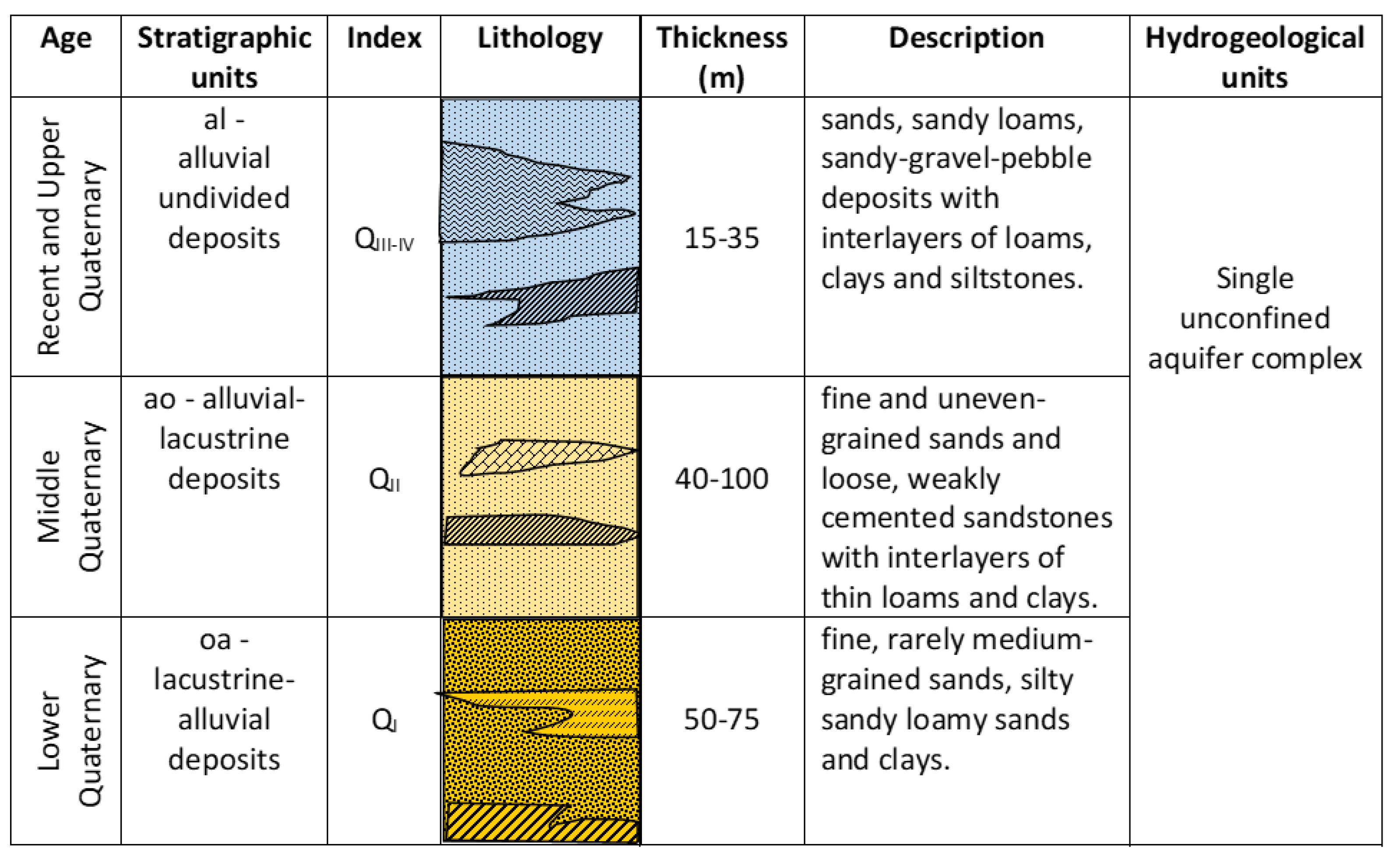
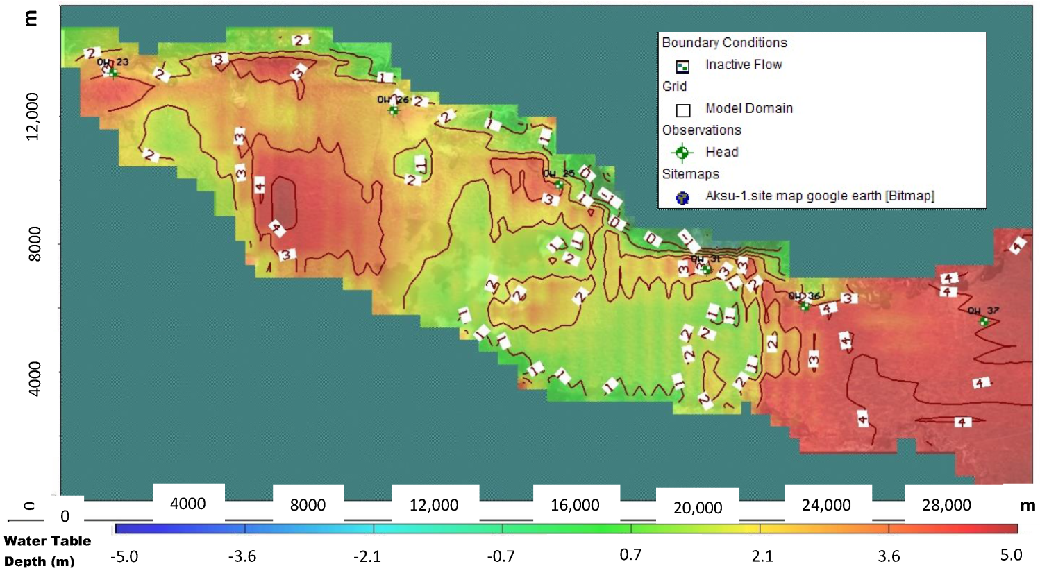
The groundwater depth at the Aksu research site is less than 7 m deep, whereas during the development of groundwater-based distant pasture infrastructure, the following subaquifers of the upper aquifer section (Figure 2) were found to be suitable for distant pasture irrigation and livestock watering:

• an alluvial undivided recent and Upper Quaternary deposits aquifer (al Q_III–IV), consisting of sands, sandy loams, sandy-gravel-pebble deposits with interlayers of loams, clays and siltstones. The aquifer thickness varies from 15 to 35 m. The groundwater level depth varies from 3 to 5 m in the spring and from 5 to 7 m in the summer. The groundwater salinity practically does not change during the year and is up to 1 g/L with a predominant bicarbonate-sulfate sodium composition. The hydraulic conductivity coefficient is 3.15–4.5 m/d. The water discharge rate of wells during the airlift pumping test was 0.6–0.9 L/s, with groundwater level drawdown equal to 1.5–2.5 m.
• alluvial-lacustrine Middle Quaternary aquifer (ao Q_II) deposits, consisting of fine and uneven-grained sands and loose, weakly cemented sandstones with interlayers of thin loams and clays. The aquifer thickness increases from 40 m closer to the Aksu riverbed to 100 m in the direction of the Akozek River. The groundwater level depth varies from 3 to 4 m in the spring and from 4 to 7 m in the summer. The groundwater salinity ranges from 1 to 2 g/L in the northern part of the study area to 2 to 2.5 g/L near the Akozek River. Groundwater has the prevailing sodium bicarbonate chloride and sodium bicarbonate chloride composition. The hydraulic conductivity coefficient of the deposits is 1.6–2.5 m/d. The water discharge rate of wells during the airlift pumping test was 0.2–0.9 L/s with groundwater level drawdown equal to 1.0–3.2 m.
• lacustrine-alluvial Lower Quaternary sediments aquifer (oa Q_I), consisting of fine and fine, rarely medium-grained sands and silty sandy loamy sands, located in the experimental area in the easternmost part, with hilly ridge eolian relief. The aquifer thickness varies from 50 to 75 m. The groundwater level depth varies from 2 to 5 m in the spring and from 3 to 7 m in the summer. The groundwater salinity ranges from 1 to 2 g/L with a predominant bicarbonate sodium chloride composition. The hydraulic conductivity coefficient of the deposits is 1.3–1.5 m/d. The water discharge rate of wells during the airlift pumping test was 0.5 L/s with groundwater level drawdown equal to 2.0 m.

All the above-described aquifers are hydraulically connected and represent a single, unconfined aquifer complex.

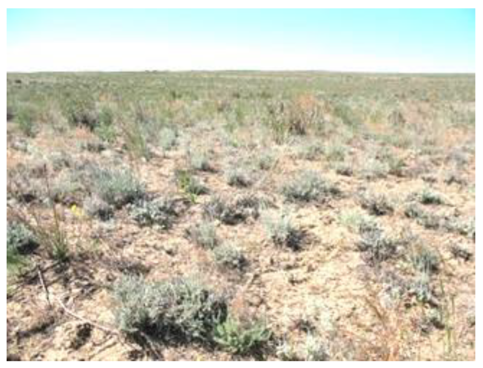
Grass groups and reed communities are widespread in the Aksu River floodplain and low terraces, as well as to a lesser extent at the Akozek River. Over hilly ridges of aeolian relief, Erkek formations with wormwood, as well as a reed–rank–wormwood association, were developed, making them permissible for distant pasture grazing. 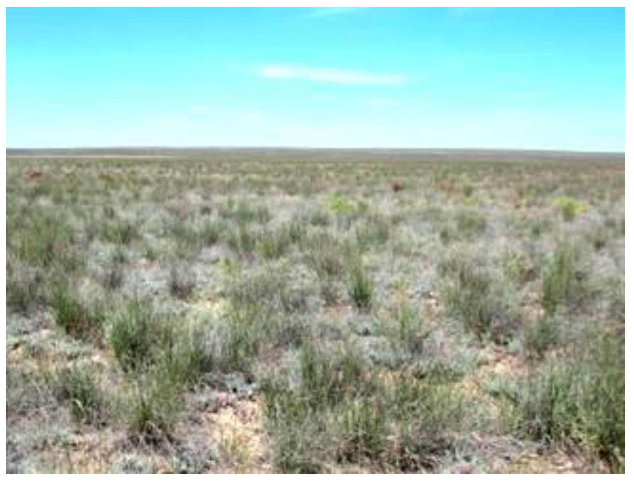Erkek formations are represented by two vegetation types: where the groundwater depth does not exceed 3 m, the first community coverage is 30–35% in spring and 40–45% in autumn, consisting of wheatgrass–wormwood with reed and patches of wheatgrass (Figure 3), and where the groundwater depth is more than 4.5–5 m, the second community coverage is 30–40% in spring and 30–35% in autumn, consisting of a wheatgrass–white–wormwood community with teresken (Krascheninnikovia ceratoides (L.)) or teresken–wormwood with wheatgrass (Figure 4).

The vegetation cover density varies from 400 to 700 kg/ha. for a pasture fodder period of 200–220 days. The Pasture Use Schedule is based on seasonal farm animals’ migration routes, starting from the 1st term of March until the 2nd term of May, from the 1st term of June to the 2nd term of August and from the 1st term of December to the 2nd term of February. The extent recommended for distant pastures is 32,450 hectares in total area, and the recommended permissible livestock number on pasturelands is 3245 heads.

The average livestock keeping water consumption used for calculations is 50 L/day/head. The total water demand for watering livestock in the pasture period is 63,318 m³, and the daily water consumption for keeping livestock on pasturelands is 302.4 m³/d. Pastures’ groundwater supply is carried by autonomous watering points equipped with hybrid wind–solar electro power stations and borehole pumps [25].

2.2. Research Methodology

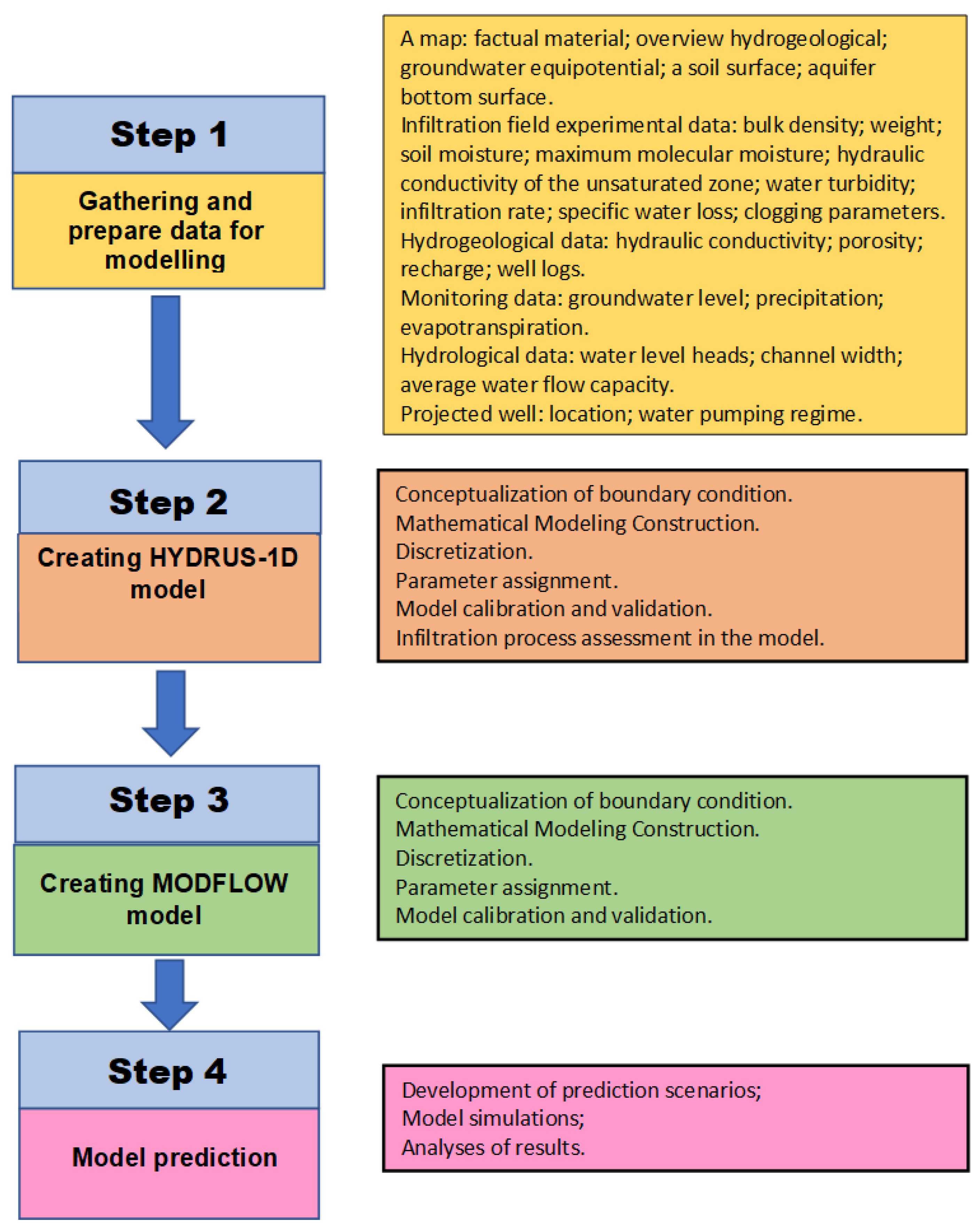
This study integrates hydrogeological surveys and field experiments with saturated and unsaturated soil strata water movement models. The conceptual working process developed in the present study is shown in Figure 5.

In the first step, all available data needed for modeling were collected and arranged as a Geographical Information System Data Base (GIS-DB). The data were obtained from official Kazakh hydrogeological survey reports, the personal communication of the government program and field research in the area [19]. In the second step, a reasonable assumption that the flow from the mini pools to the aquifer vertically enabled the use of the HYDRUS-1D model that was created to evaluate the infiltration and clogging processes at the infiltration mini pool and in the unsaturated zone. The one-dimensional model characterized the cross-section from the soil surface to the unconfined groundwater level depth. The HYDRUS-1D model results made it possible to characterize the water recharge flow rate into the aquifer. MODFLOW software’s basic requirements for model construction included area discretization of lithology, boundary conditions, observed groundwater heads and HYDRUS-1D model results (step 3). Since the system consists of one aquifer layer and the HYDRUS-1D supplies the input to this layer, a 2D MODFLOW model is sufficient. After the MODFLOW model calibration and validation, model predictions were performed (step 4). Based on water withdrawal potential scenarios, the calibrated model parameters were used as a starting point for groundwater drawdown estimation in the pumping wells.

2.3. Research Procedure

The modeling database included the following:

• hydrogeological map at the 1:200,000 scale, a groundwater equipotential map, a soil surface map and the unconfined aquifer bottom surface map.
• infiltration field experiment data, percolation tests in the experimental pits, infiltration tests from the mini pools and pumping tests; soil and water sampling supplied: the mechanical components of the soil profile; volumetric soil moisture; bulk density; water turbidity; infiltration flow rate; thickness of the clogging layer formed in the infiltration mini pools bottom.
• data on the hydraulic conductivity coefficient, porosity and recharge of the aquifer were obtained from infiltration tests and field studies carried out on-site at different times.
• groundwater level monitoring through the observation well network (Figure 1) from 2018 to 2020.
• precipitation and evapotranspiration data, by monthly average in individual zones, based on the vegetation distribution, for the period from 2018 to 2020.
• data on water level heads, channel width and average water flow capacity in the Aksu and Akozek rivers in separate sections within the research site.
• water pumping regime from projected wells on pasture areas.

The modeling aim was to solve the following tasks:

• Groundwater and unsaturated zone flow numerical models’ development and calibration; with a focus on the upper phreatic unconfined aquifer, within the research site hydrogeological and geographical conditions.
• Predictive assessment of groundwater level drawdown and the balance of groundwater flow components for pumping well water intake conditions at watering points.
• Infiltration rate assessment for artificial recharge of the phreatic unconfined aquifer from infiltration pools.

2.4. Development of the Unsaturated Zone Water Movement Model

The water movement model in the upper unsaturated soil layer and down to the groundwater level was created in HYDRUS-1D software [26]. The one-dimensional model characterizes the groundwater depth cross-section.

A basic mathematical model of the one-dimensional water movement for an unsaturated soil state is described by the following equations:

∂W/∂t = ∂/∂x[K(W) (∂H/∂x)] − E(W,x)

(1)

K(W) = ƒ(Ks,W)

(2)

where:

• W—Volumetric Moisture
• H—Suction
• K(W)—Hydraulic conductivity of unsaturated soil state
• E—Plant root moisture absorption function
• t—Time

The Van Genuchten-Mualem (no hysteresis) single porosity model [27] was used as the hydraulic model. The clogging phenomenon was taken into account by adding the silty clay layer 4 cm thick with a hydraulic conductivity coefficient equal to 0.0048 m/d to the model soil profile.

2.4.1. Modeling of the Infiltration Process

The initial data for the infiltration process modeling were the in-situ test carried out at the Aksu experimental site [19]. Two infiltration process variants were modeled using HYDRUS-1D software. The first is simulated infiltration from the soil surface to the groundwater level, and the second is river water infiltration from the infiltration mini pool, with a clogging process development at the bottom of the pool. The main goal of the modeling was to study the water infiltration process in the unsaturated zone and estimate the possible recharge to the upper aquifer from atmospheric precipitation filtration and/or surface water and/or irrigation.

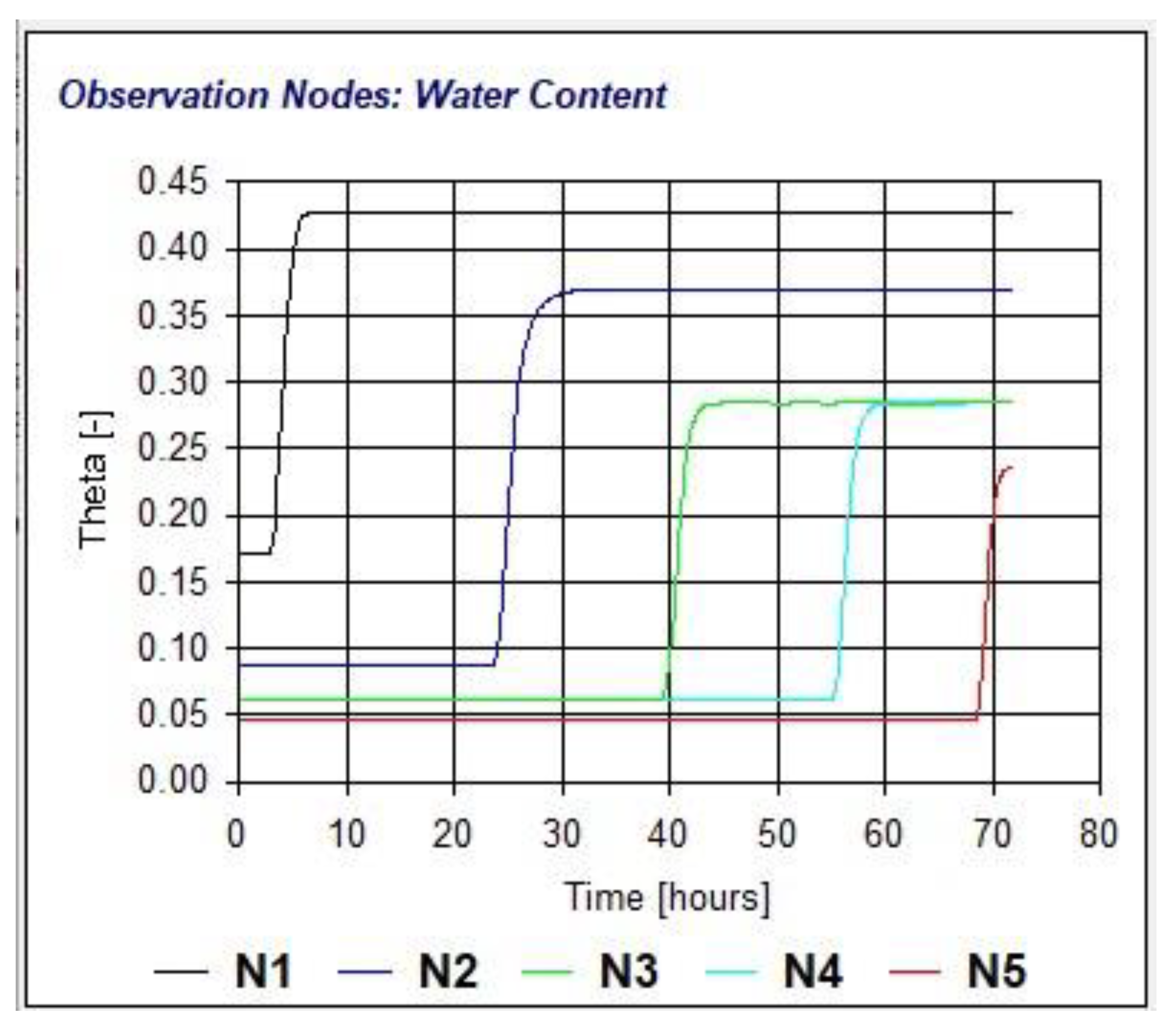
2.4.2. Creating a HYDRUS-1D Model from the Soil Surface to the Groundwater Level

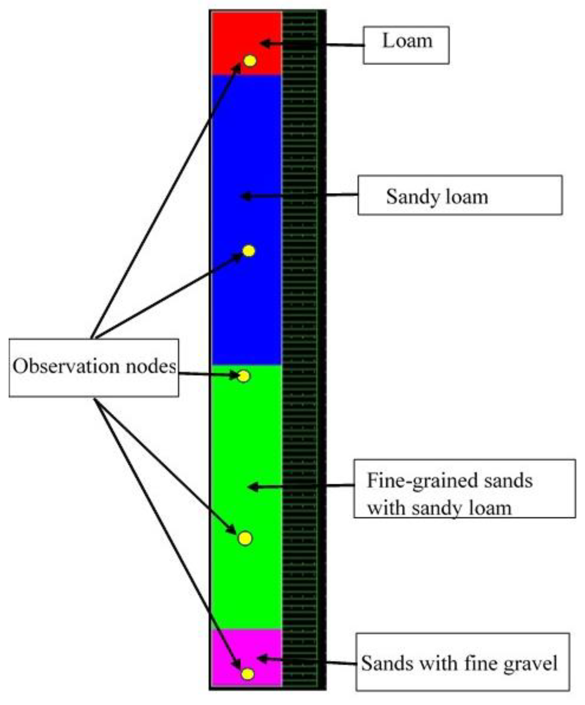
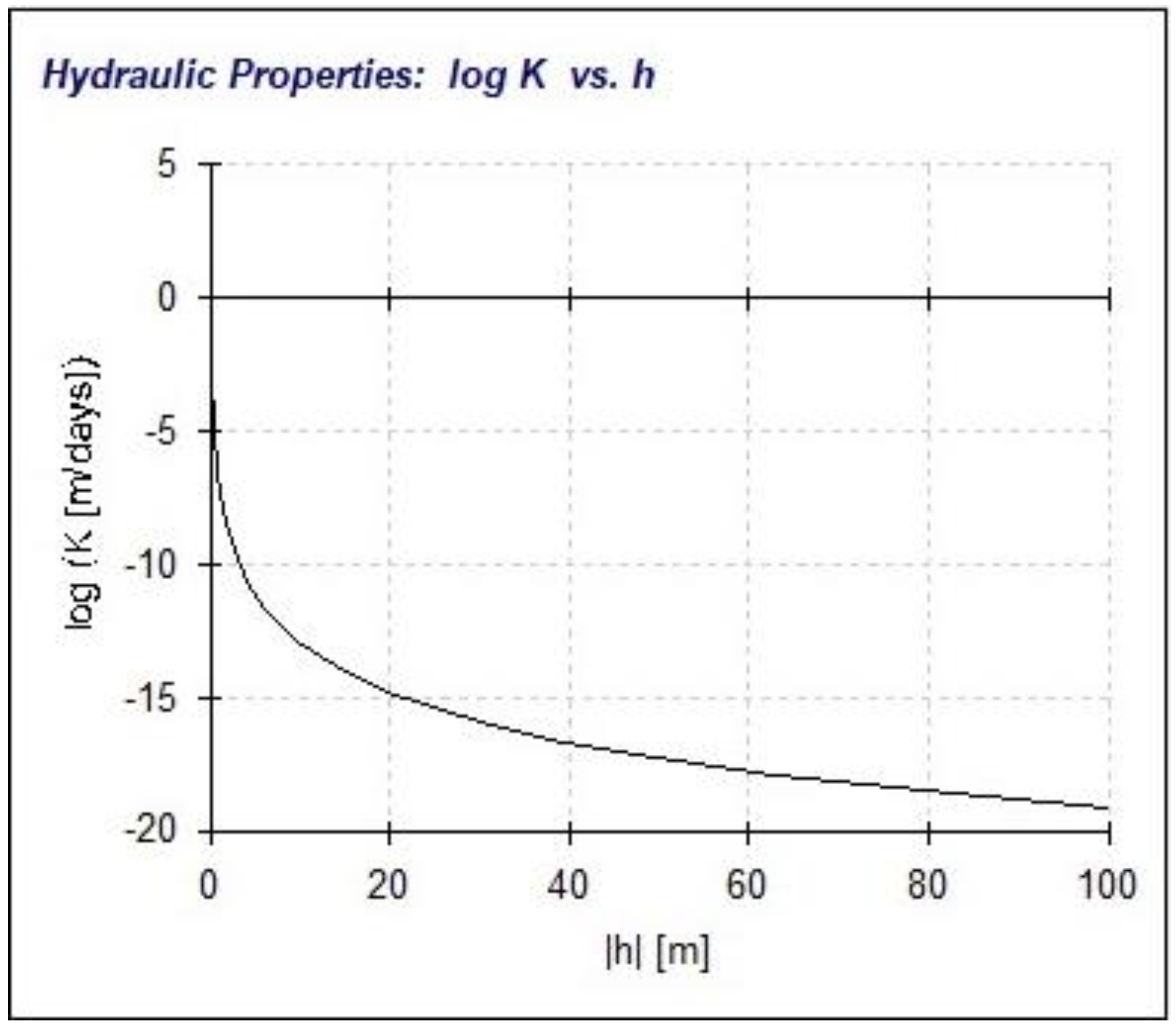
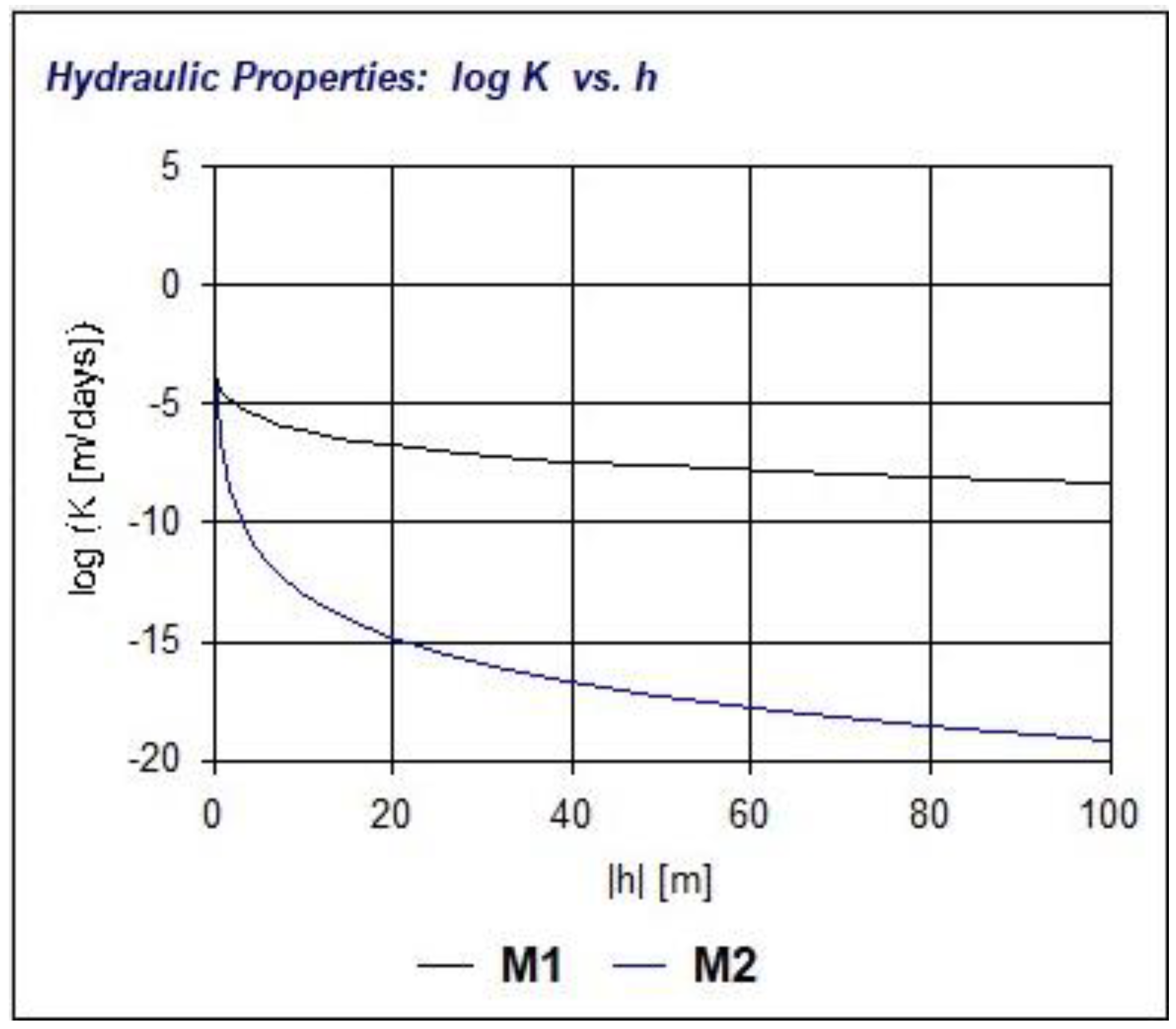
Based on the groundwater level maximum depth during the field experiment, the model soil profile thickness was taken as 300 cm. The calculated points on the profile were set uniformly along the soil profile depth in 3.0 cm steps. The soil profile was divided into four sections by the sediment’s lithology. The first section (upper) to a depth of 30 consists of loam. The underlying layer (2nd section) to a depth of 160 cm is represented by sandy (light) sandy loam. To a depth of 270 cm, the section contains fine-grained sands with sandy loam (3rd section). The last 30 cm of the soil section (Section 4) consists of sands with fine gravel inclusions. These profile sections were characterized by the following hydraulic conductivity coefficient values under full saturation conditions: 1.04, 4.42, 14.59 and 29.7 cm/h, respectively (Figure 6).

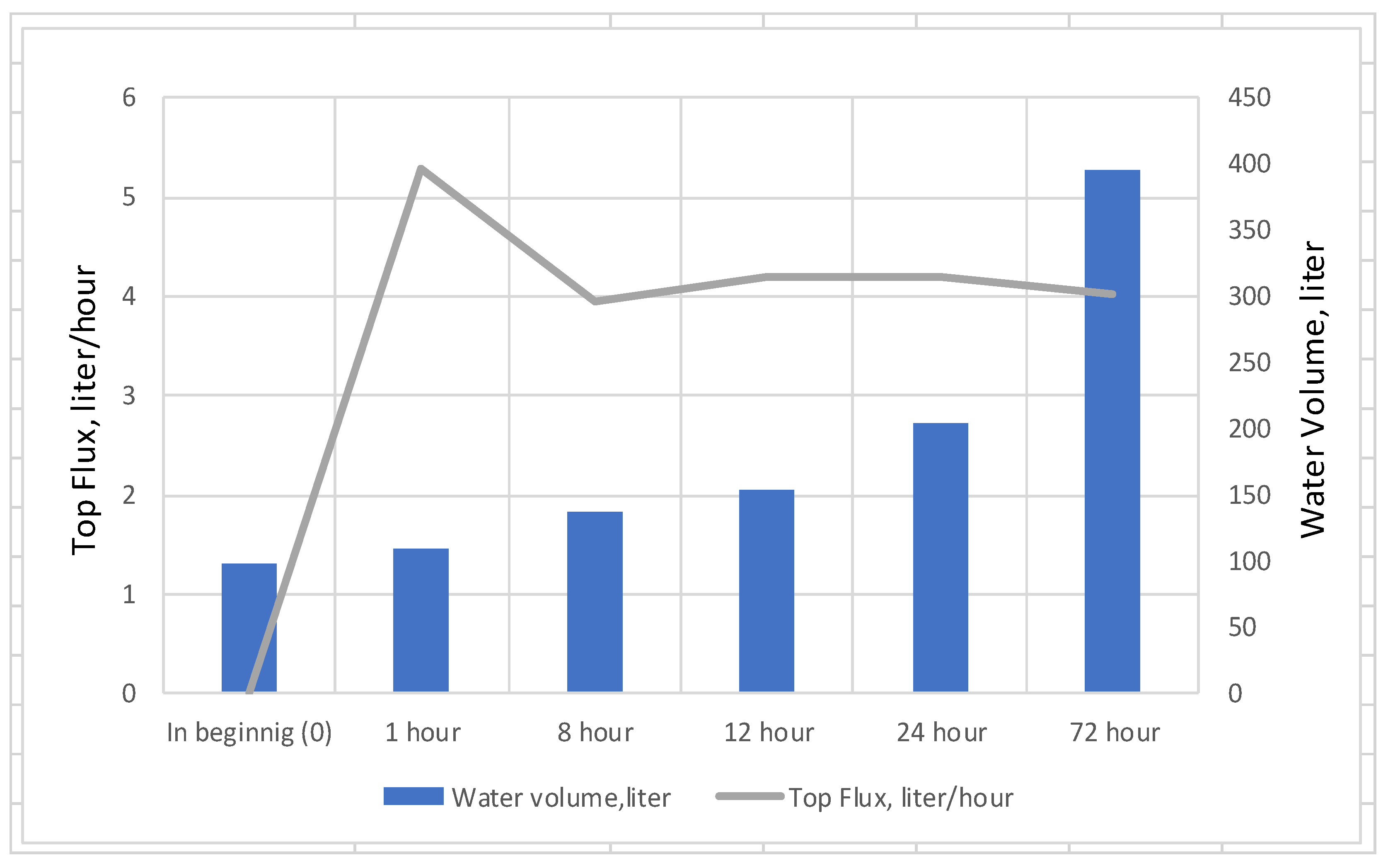
To the upper model boundary, the constant time pressure is set to 0 (zero) for simulating a water-saturated surface (Constant Pressure Head). At the model’s lower boundary, free filtration (drainage) conditions were set, corresponding to the thickness of the soil profile and equal to −300 cm. The total model duration is 72 h in calculation intervals of 0, 1, 8, 12, 18, 24 and 72 h from the starting point that was selected following the measurements performed during the experiments. Observation points were set at a soil profile depth of 30, 100, 160, 230; 295 cm relative to the soil sampling depth and field measurements.

2.4.3. Creating an Infiltration Model of the Experimental Mini Pools

The one-dimensional filtration flow process in the unsaturated zone comprised data on the lithological description, filtration capacity and other parameters. Based on mini pool 1 infiltration test results, two options were modeled: the first was water infiltration from the pool without a colmatation layer, and the second was infiltration with a 4 cm thick clogging layer. The soil profile lithological composition and the model boundary conditions were the same as those in the field experiment. Based on the groundwater maximum depth from the infiltration mini pool during the initial experimental period, the soil profile thickness in the model was 200 cm. The profile sampling points consisted of sands and fine gravel, which were set evenly with 2.0 cm steps. The soil profile hydraulic conductivity coefficient under saturation conditions was equal to 7.128 m/d, and the clogging layer hydraulic conductivity coefficient represented a 4 cm thick silty clay layer and was set as 0.0048 m/d. At the model’s upper boundary, a constant pressure head was set equal to +1.8 m, simulating a water column above the bottom of the pool. At the lower model boundary, time-varying pressure head conditions (Variable Pressure Head) were set, simulating the groundwater level time-varying depth. The model’s final time was 244 days, with calculation intervals of 0, 1, 5, 20 and 244 days from the starting point. Observation points were set at the depth of the soil profile: 0.1, 0.5, 1, 1.5 and 1.9 m.

2.5. Development of the Upper Unconfined Aquifer Groundwater Flow Model

By the Quaternary unconfined aquifer model scheme, the mathematical groundwater flow model is described by a partial differential equation of two-dimensional groundwater flow through porous material in a mono-layer geo-filtration system of the unconfined aquifer as follows:

∂/∂x[Kx(Hx − ηx)(∂H/∂x)] + ∂/∂y[Ky(Hy − ηy)(∂H/∂y)] ± W = Sy(∂H/∂t),

(3)

where Kx and Ky = hydraulic conductivity along the x- and y-coordinate axes, respectively, which are the principal permeability directions; H = potentiometric head; ηx and ηy = elevation of the bottom of the unconfined aquifer along the x- and y-coordinate axes; W = fluxes that represent recharge, evaporation and pumping; Sy = specific yield of the porous material; and t = time.

Equation (3), with the following boundary conditions and a specific initial head condition, provides a mathematical representation of a groundwater flow model in the study area. The model boundary conditions are represented as head and flow. To represent the research site spatial variability, the area was overlain by a grid, with each cell representing a cell centerpoint. The grid was applied to the layer characterizing the hydrodynamic and geological changes through the soil cross-section. The distant pasture groundwater model was constructed using Visual MODFLOW, a three-dimensional groundwater flow simulation integrated computer program package [28].

2.5.1. Model Representation

Under the adopted mathematical model, the computer model consisted of one horizontal layer. The aquifer in the model is represented by undivided recent and Upper Quaternary sediments, comprised of sands, sandy loams and sandy–gravel–pebble deposits with interlayers of loams, clays and siltstones. The total aquifer thickness ranges from 50 to 110 m, with a gradual increase to the south from the Aksu River to the Akozek River. The model’s lower boundary (base) runs along the top of low-permeability argillaceous Middle and Lower Quaternary deposits, as well as the Neogene Ili formation, represented by dense clays, which are the regional aquiclude that was adopted as an impermeable boundary.

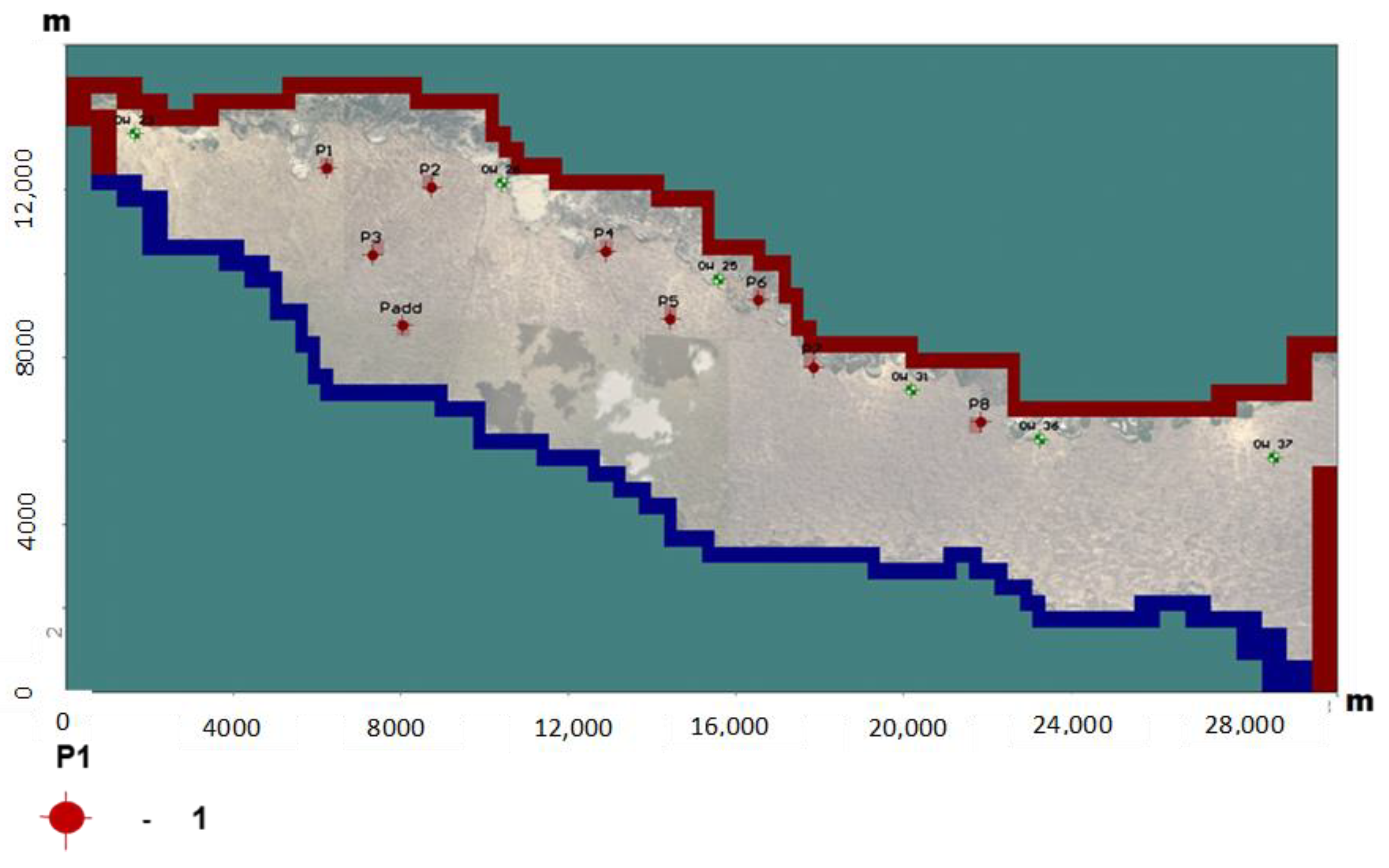
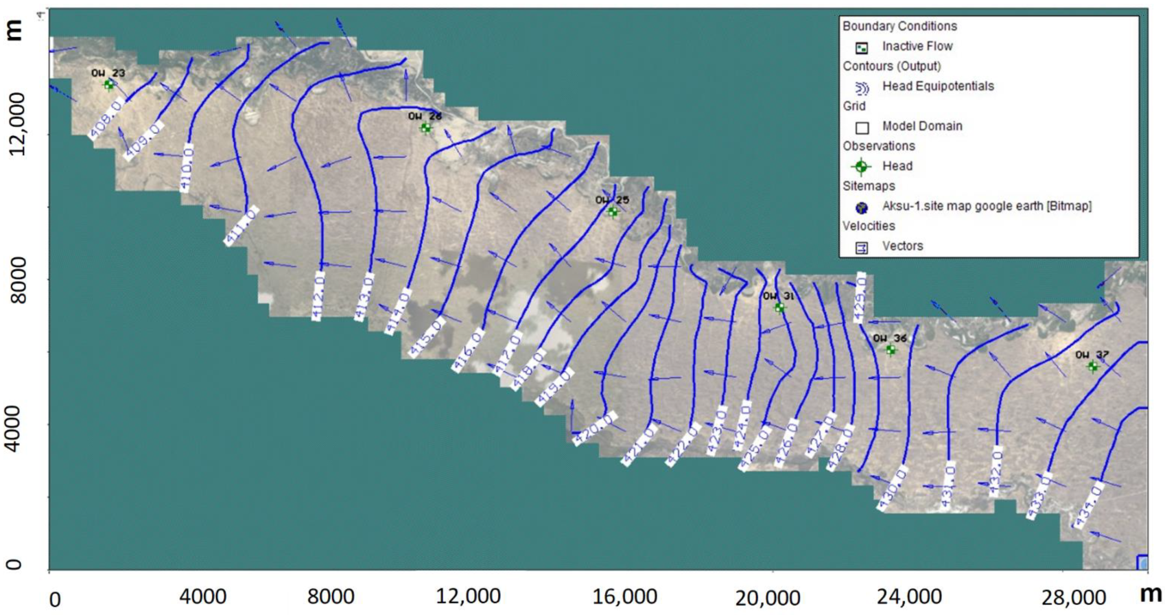
A geo-filtration computer model was created within the following boundaries (Figure 7): The northern boundary is represented by the Aksu riverbed; the southern boundary is the Akozek River; the eastern boundary is an ordinate in an alignment perpendicular to the Aksu River buried bed; and the western boundary is the Akozek River mouth, which flows into the Aksu River.

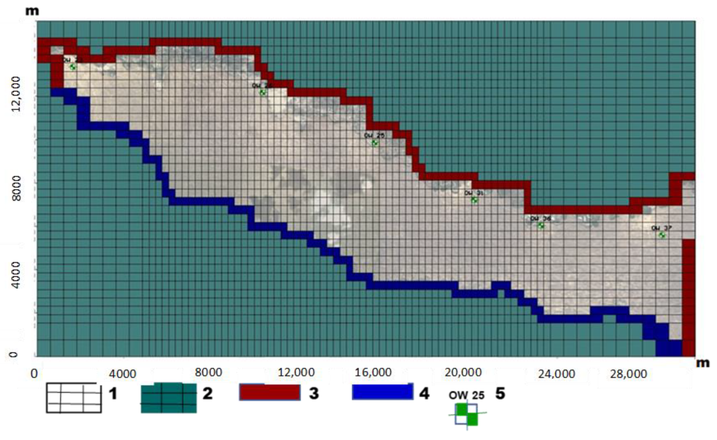
The model area was divided into a rectangular grid with dimensions of 81 by 37 computational cells (2997 cells). The grid steps along the axes are irregular and vary from 590 to 310 m along the X-axis and from 740 to 370 m along the Y-axis. Thus, the computing unit’s maximum area was 0.4366 sq. km, and the minimum is 0.1147 sq. km. The computational grid minimum step was specified where it was required to obtain detailed information, and the grid maximum step was specified in the eastern and western regions of the experimental site model (Figure 8).

The model’s coordinates benchmark was in the rectangular region lower left corner (45°46′14″ N and 78°34′35″ E). The geo-filtration active area is highlighted by defining inactive blocks outside its external borders.

The model boundary conditions were set as follows (Figure 8):

• flow rate of groundwater entering the model through the eastern border.
• discharge/groundwater recharge to/from the Aksu and Akozek rivers.
• rainwater infiltration from April to November.
• evapotranspiration or evaporation from the groundwater level.

The flow enters the model through the model’s eastern boundary, which was set as boundary conditions of the first type (BC-I) with pressure head values, following the equipotential map at the beginning of 2018. Considering that, in the long-term period, these pressure head values hardly changed over time, the head values were constant for the entire model duration. Bearing in mind the hydraulic connection between the Aksu River water level and the groundwater level, the model northern boundary (Aksu River) was simulated as a linear boundary with a pressure variable along the river course as a boundary condition of the first type (BC-I). The pressure head values along the border were taken to be equal to the long-term average values of the water level in the river (in absolute marks) and remained constant for the model calculations period.

The model southern boundary along the Akozek River was correlated to the intermittent runoff flow during the year and set as boundary conditions of the third type—“River” (BC-III) under the “Visual MODFLOW Pro” software package requirements. These boundary conditions simulated the groundwater discharge or recharge from a river or into a river. Groundwater recharge from the river (feeding) or river recharge from the groundwater (unloading) was calculated according to the difference in river water level heads and the river channel bottom elevation in the model boundary cells.

The Visual MODFLOW Evaporation Package was used to simulate the groundwater table contribution to capillary rise, evaporation and evapotranspiration. The capillary fringe boundary condition assumes a linear relationship between evapotranspiration potential and the groundwater level. Groundwater withdrawal was calculated for each time step for the specific groundwater level depth. The evapotranspiration maximal value was calculated for the water level at the surface as the surface water evaporation value. With the groundwater level decreasing, the evapotranspiration flux linearly decreased up to a groundwater level, where the evapotranspiration flux was null [29]. The initial input values were based on local meteorological evaporation data and applied uniformly over the model area with a critical depth of 1.5 m and corresponded to the prevailing lithological composition of the unsaturated zone. The mean long-term evaporation values were set for March to November by zones aligned with the vegetation cover distribution and varied from 63 to 72 mm/year for November and from 1215 to 1989 mm/year in August.

Groundwater spatial rainfall recharge was set in the by-zones to the Visual MODFLOW Recharge Package. The initial recharge value was set at 15% of the total monthly precipitation, considering the groundwater table depth in the area and the high summer temperatures. It was also assumed that, in the winter period from December to March, there was no groundwater recharge due to direct rain infiltration, and 25% of the total winter precipitation was added to the groundwater recharge in April due to melting water infiltration. The total groundwater recharge value was subsequently adjusted at the calibration and model validation stages.

The model time step was set in days from the model calculation beginning (start time—0 days), which was set to 1 January 2018—the beginning of the observations. The model calculation ending time was 3650 days (10 years) to provide future prediction modeling. Intermediate time steps were set automatically by the program depending on the time of boundary condition changes and observation periods (stress periods). The groundwater head equipotential map for January 2018, created by interpolating values of the groundwater heads, measured in the observation wells and on the boundary conditions of the 1st type, which was applied as the model initial head conditions.

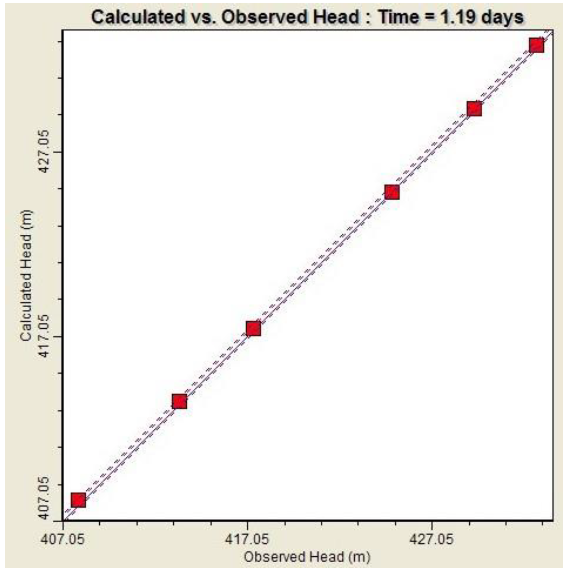
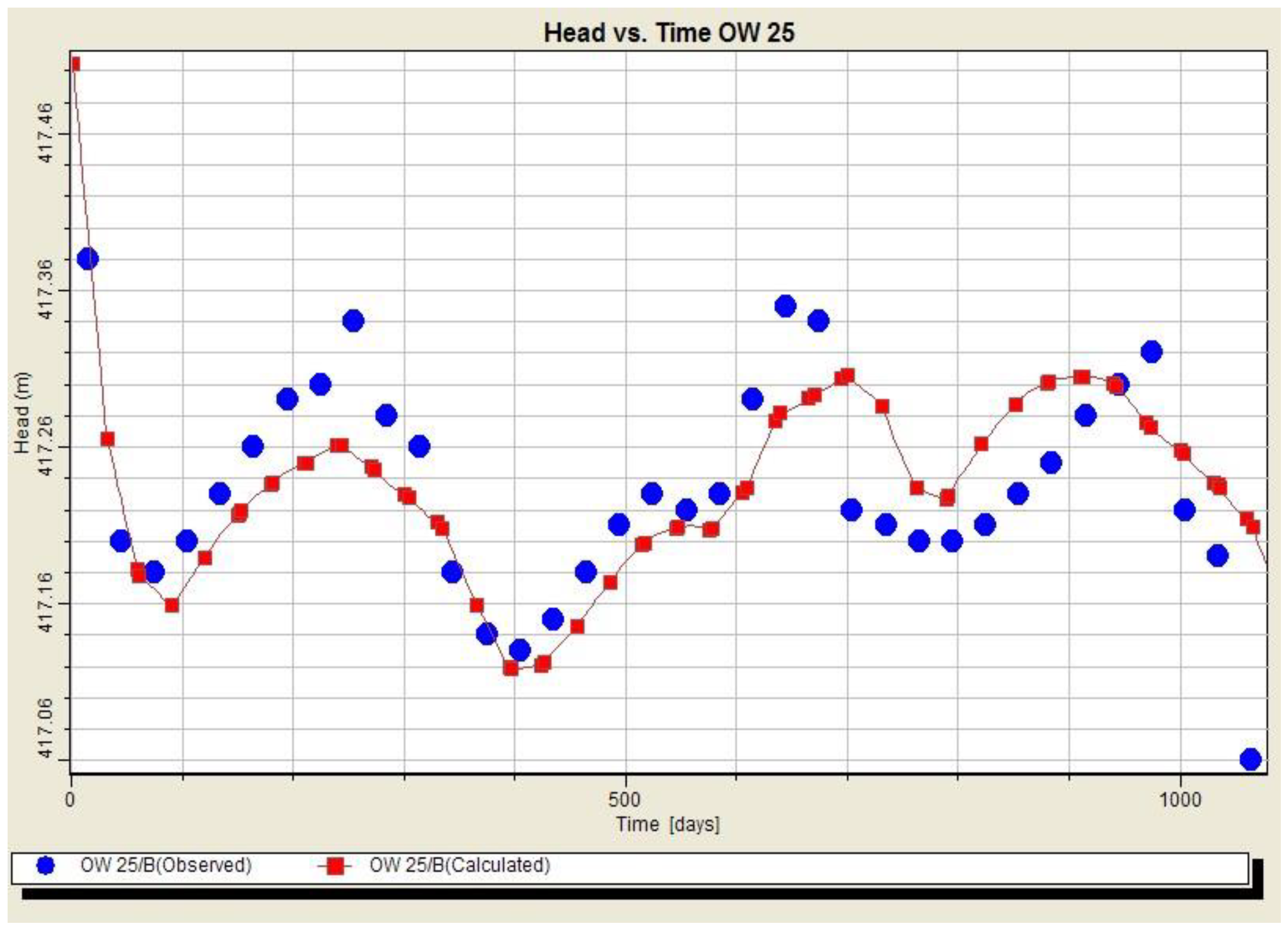
2.5.2. Methods: Model Calibration

During calibration, the model was adjusted until it closely simulated the measured historical values of the modeled system. The model layer hydraulic conductivity values, aquifer storage coefficients and recharge were adjusted, and the water balance was evaluated. The model ran from 1 January 2018 to 31 December 2020, during which the actual system behavior was observed. Wherever the simulated water level and pressure behavior did not match the observed behavior, careful adjustments were progressively made to the model hydraulic conductivity and recharge value layers assigned to characterize the relevant cells. Model calibration was continued until an acceptably close match between simulated and observed behaviors was achieved. Match “Acceptability” was mathematically determined once the overall calibration accuracy could be quantitatively assessed. The water balance coincidence elements obtained from the field measurement data and calculated for the model were limited by their hydrogeological reliability. To assess the model calibration accuracy, a groundwater level regime in six observation wells was used. Consequently, 0.2 m was set as the maximal coincidence accuracy level, owing to the detailed lithological section schematization and the spatial discretization accuracy. As the amplitude of groundwater level fluctuations in the observation wells reached 0.8 m, the declared solution accuracy should not exceed 25%, and in terms of groundwater, the budget was defined as ±5%. To understand which parameters are most or least likely to affect the model results, a “sensitivity analysis” was carried out as part of the calibration process. The model calibration was carried out for the no-steady-state (time-varying) phases.

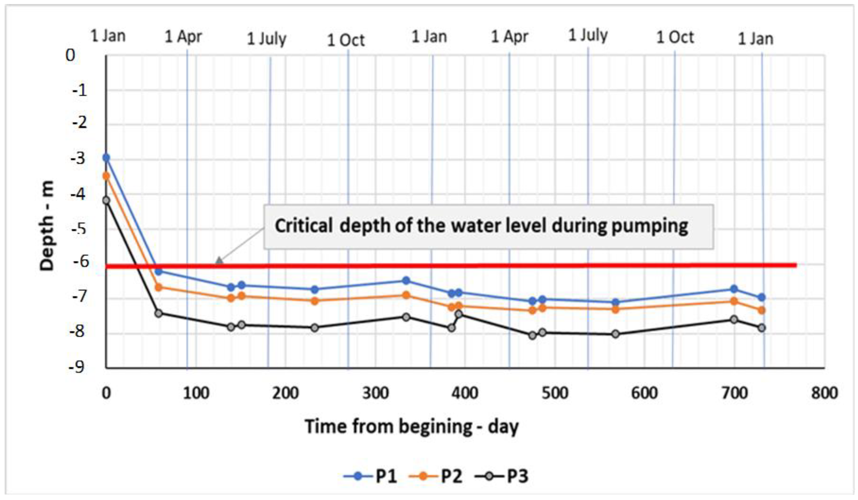
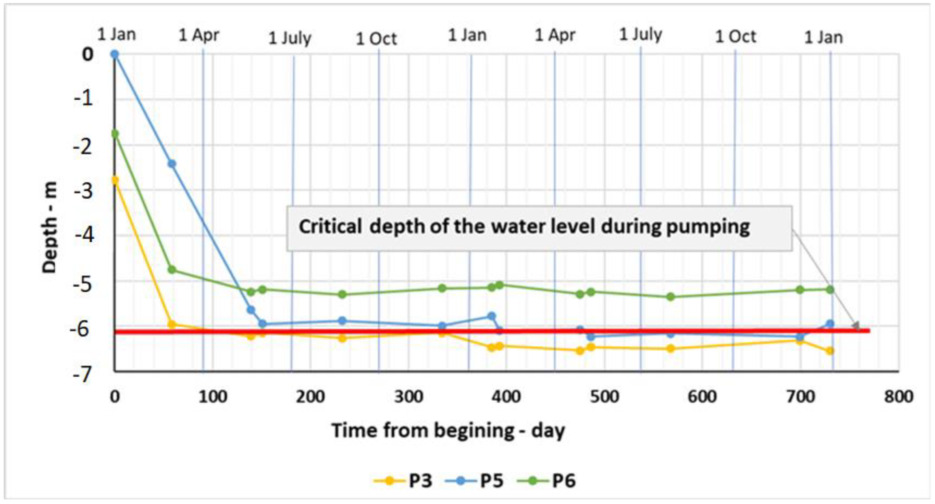
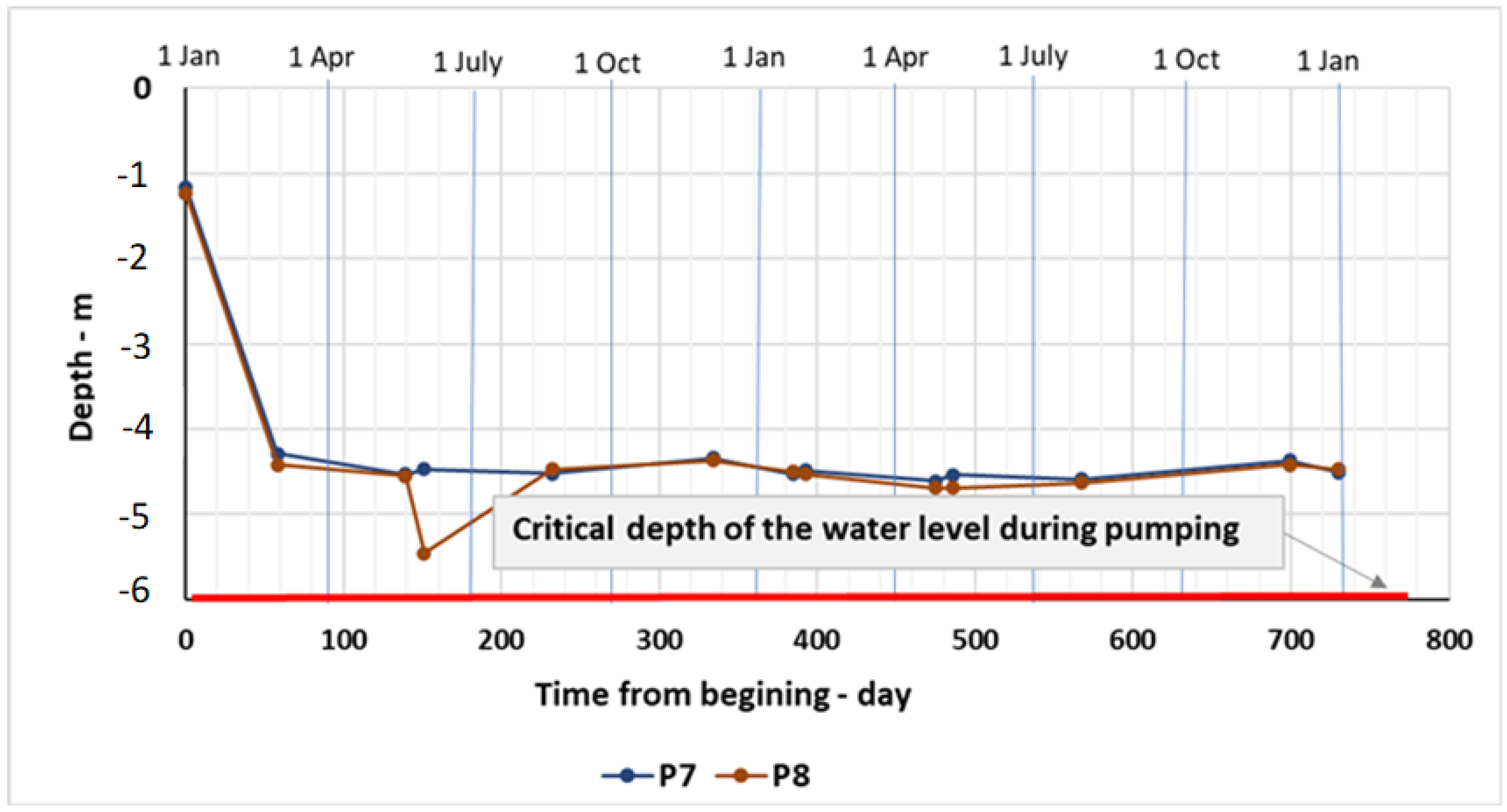
2.5.3. Methods: Model Predictions

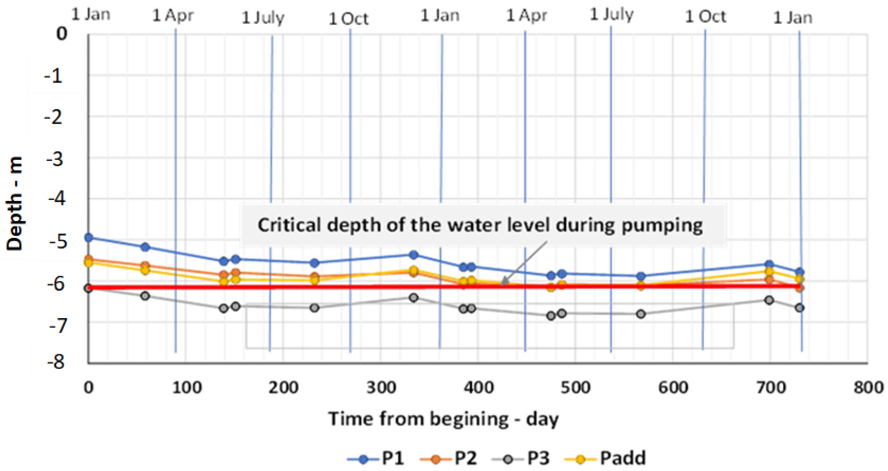
The initial prediction model data were set to a common datum, enabling calibration and validation. The calibrated model was applied to simulate and predict groundwater decrease scenarios with production well drawdown in projected locations. For a given water withdrawal mode, the model enabled comparing and obtaining values of maximum permissible groundwater level drawdown during pumping. Based on the projected watering point pumping equipment technical and economic indicators, the maximum permissible water level depth in the wells was determined to be 6 m from the soil surface. Considering that the simulated area is a natural cattle pasture on which the construction of engineering structures is not envisaged in the future, their impact on the predicted drawdown in groundwater levels during pumping was not considered. The influence of various dewatering or recharge engineering construction on groundwater balance and groundwater drawdown is discussed in detail in the works [30,31,32,33]. The predicted drawdown exceeding the permissible drawdown indicates that the specified water withdrawal regime and water level in production wells can be attained by artificial infiltration basins that prevent the need for additional production wells in the pasture area.

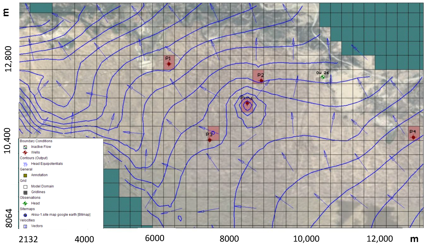
The eight production wells distributed over the research area are considered: the fodder area fund in the pasture period; the number of livestock; and the pasture use schedule, which establishes the seasonal farm animal movement routes (Figure 9). The water withdrawal from the production wells was equal for all wells. The pumping flow rate was selected from the calculated water demand, seeing the pump’s technical characteristics, and was set equal to 288 m³/d during the water withdrawal during the water consumption season. This flow rate was set during the following terms: from 1.03 to 20.05 (81 days); from 1.06 to 20.08 (81 days); and from 1.12 to 20.02 (51 days). In between these terms, a flow rate of 95 m³/d was set as the maximal operation of the wells outside the water consumption season.

The calibration was carried out for three years. The prediction was performed for two years. The beginning of the model prediction corresponded to the end of the calibration model period on 31 December 2020 (1095 days), and the end of the model calculation corresponded to 1825 days.

The Theis solution [34] was used to adjust the model cell size to the real well diameter, enabling transition cuts (corrections) of computing cell area to the real well size and the modeled to actual drawdown comparison.

2.6. Modeling Limitations

Groundwater flow models are necessarily simplified mathematical representations of complex natural systems. As such, there are limits to the accuracy with which groundwater systems can be simulated [35]. The model error commonly stems from practical limitations of grid spacing, time discretization, parameter structure, insufficient calibration data and the effects of processes not simulated by the model. Horizontal discretization affects MODFLOW model predictions, particularly where large hydraulic gradients are to be expected near pumping and injection wells where hydraulic gradients are steepest. Local-scale modeling is one of the ways to resolve this issue. Another way is to adjust the hydraulic gradient value by relating the model cell size to the real pumping well diameter. However, the increase in spatial discretization is associated not only with high computational costs but is also largely limited by the insufficient detail of the initial information. Certain limitations on the accuracy of predictive model calculations are also imposed by the specified boundary conditions associated with the lack of information on their changes in the prediction period [36]. In this regard, the flow rate of groundwater entering the model through the eastern border, the relationship of groundwater with the Aksu and Akozek river runoff and rainwater infiltration for the prediction period were set unchanged and obtained as a result of model calibration. The calibration-constrained uncertainty analysis was used to quantify the effect of horizontal hydraulic conductivity, modeled water table recharge and specific storage on model predictions. The numerical results of the flow model have an associated, but unquantified, uncertainty. While it is possible to quantify model prediction uncertainty, that analysis is not included within the scope of this research. A sense of model uncertainty will develop as conditions are monitored in the future and compared to model predictions. For these reasons, continued monitoring of hydrologic conditions at the Aksu experimental site is crucial.

3. Results and Discussion

3.1. HYDRUS-1D Model Simulations

3.1.1. Infiltration from the Soil Surface to the Groundwater Level

In the first stage, various hydro-physical parameter combinations of the model were selected according to the soil’s hydraulic conductivity coefficients for the HYDRUS-1D soil catalog under saturated conditions. The soil profile lithological description and the hydraulic conductivity coefficients as basic criteria were obtained during the water percolation tests in the pits. When the computational process in certain hydro-physical combinations lacked convergence, the best hydraulic conductivity coefficients were taken as saturated conditions of 0.3, 1.6, 3.5 and 7.1 m/d for the model’s 1, 2, 3 and 4 lithological layers (areas), respectively, which were found to agree with the experimental test averaged values.

At the second modeling stage, the soil’s hydro-physical parameters and the unsaturated zone water flow balance components were analyzed. An inner ring area of 0.04 m² was used to calculate the filtration flow volumetric components. The change in volumetric soil moisture with time at different soil profile depths is given in Figure 10. Calculations have shown that, after infiltration began, the soil moisture throughout the soil profile section reached its maximum full saturation value at approximately 70 h. At the same time, there is a certain delay in the initial time of the soil’s volumetric moisture content front advancement along the soil profile. Moreover, the increase in volumetric moisture occurs abruptly within 1–2 h, whereas the moisture values increase until complete saturation is more rapid in sands.

The complete soil profile saturation in the sandy loam layer to a depth of 1 m occurs 26 h after the infiltration starts. Throughout the soil profile, the volumetric soil moisture reaches its maximum values (complete saturation of the soil) in 3 days. A clear soil lithology boundary change exists from sands to heavy sandy loam with higher volumetric moisture content at full saturation. As the pressure decreases, the soil’s volumetric moisture content increases nonlinearly and reaches its full moisture saturation, at which the suction pressure value is zero. The soil moisture transfer coefficient is nonlinear and dependent on suction pressure and the soil profile lithology. Under full saturation conditions, the soil moisture and soil moisture transfer coefficients increase in parallel and reach the hydraulic conductivity coefficient values of the aquifer. For dry soils, the soil moisture transfer coefficient approaches zero. Moisture transfer balance component calculations made it possible to estimate the unsaturated zone runoff infiltration volume through the soil profile and to characterize the aquifer runoff recharge (Figure 11) and the model’s accuracy and reliability.

In three days, the soil profile water volume increased from 98 L to 396 L, whereas approximately 100 L were filtered during the first day. At the same time, the flow rate through the profile upper boundary increased within the first hour from zero to 5.3 L per hour and then began to gradually decrease until, after 8 h, it stabilized at a level of approximately 4 L per hour.

3.1.2. Infiltration from the Experimental Mini Pool

Infiltration without a Clogging Layer

Model calculations showed that, after infiltration began, the soil moisture in the entire sandy soil profile depth reached its full saturation value within approximately one day. The soil moisture transfer coefficient (on a logarithmic scale) dependence on the suction pressure (hydrostatic head) during infiltration from the mini pool without a clogging layer (Figure 12).

Infiltration with Clogging Layer Modeling

With a clogging layer, the volumetric soil moisture dynamics over time at different soil profile depths were found to be rather stable. The soil moisture transfer coefficient (on a logarithmic scale) dependence on the suction pressure (hydrostatic head) during infiltration from the experimental mini pool with a clogging layer (Figure 13).

Model Calculations of the Balance Components

According to the simulation results, during 244 days, the total water volume entering the soil on an area of 0.45 m², without colmatation, was 95 m^3, and with a clogging layer, it slightly decreased by 0.8 m³. According to the field experiment, the water volume entering the soil was 110 m³. The infiltration flow rate calculated as a steady state model was 9.266 m³/d without clogging and less at 0.09 m³/d with clogging by the end of the infiltration period. The field experiment results showed that the infiltration rate coefficient decrease was 0.053 (or 0.49 m/d), which corresponds with the model. To maintain constant pressure, a water level of 1.8 m was kept in infiltration mini pool #1 during the field experiment. To maintain this level, a water volume of 240 m³ was used, which is more than 2.2 times the volume infiltrated through the soil profile. This difference might reflect the water loss to evaporation and horizontal dispersion from the vertical infiltration axis. The infiltration rate was 0.75 m/day and practically did not vary until the end of the experiment.

When creating infiltration basins with exposed sand deposits, the infiltration supply rate to the underlying groundwater can be approximately 10 m³/d per 1 m² of basin bottom surface. This value was used as a prediction figure for the MODFLOW model simulation. The formation of a clogging layer due to the settling of suspended particles from the Aksu River surface waters did not significantly affect the infiltration process.

3.2. MODFLOW Model Simulation

3.2.1. Model Validation and Identification

The model sensitivity analysis results indicated that, with initial values of ±15%, in specific storage and the layers’ hydraulic conductivity with initial values of ±50%, the model could recognize changes. The model was more sensitive to recharge and recharge variations and produced a reasonable fit for groundwater heads. The model calibration results represent the ratio between the model-calculated and measured averaged groundwater levels in the observation wells (Figure 14). The Absolute Residual Mean was 0.13 m; the Estimate Standard Error was 0.044 m; and the Root Mean Squared (RMS) was 0.163 m. The Correlation Coefficient between the measured and modeled groundwater levels was 0.95.

A comparison of the measured groundwater level fluctuations and the model calculated ones showed good agreement (less than ±0.2 m) between the observed and modeled results for observation piezometers (Figure 15).

A groundwater head contour map and groundwater level depths from the soil surface were created using the MODFLOW software package instrumental identification and task-solving capabilities. To characterize the research site’s hydrodynamic groundwater flow grid, groundwater head contour maps were combined with the flow paths. Maps were built for two characteristic periods of 2020: July (summer) and December (winter). The groundwater flow’s general direction coincides with the northwest relief slope in the direction along the Aksu and Akozek rivers. The flow line direction near the Aksu River characterizes the groundwater recharge areas from and to the river. The Akozek River does not practically affect the groundwater flow direction, and its confluence with the Aksu River is only in the study area. The groundwater hydraulic gradient ranges from 0.0005 in the eastern and western areas of the site to 0.0027 in the central part of the site, depending on the topographic conditions and the total aquifer transmissivity (Figure 16).

The hydrodynamic picture of the groundwater flow in winter practically does not change, and the flow direction and flow hydraulic gradient remain the same. A comparison of these maps, as well as of the equipotential map in 2018 (taken as initial conditions), indicates undisturbed groundwater flow condition formation and flow stability during the research site’s entire hydrological cycle.

The groundwater depth from the soil surface varies from 1 to 2 m near the Aksu riverbed, and at the site central part in the interfluve of the rivers, it is characterized by groundwater depths from 1.5 to 2.5 m; in the rest of the area, the groundwater depth is from 2.5 m to 4–5 m. (Figure 17). In the winter (end of December), the distribution to areas with different groundwater depths practically does not change, and the drawdown is less than 1 m, hence falling within the groundwater fluctuation range.

The groundwater balances calculated on the model as of July 2020 and December 2020 are shown in

Table 1. Groundwater-flux balance at the Aksu research site for July and December 2020. The results of the model calibration are in thousand m3/day.

Date		July 2020	December 2020
Input	Storage recharge	10.62	52.26
	Aksu river leakage (Constant Head)	5.01	4.24
	Recharge	25.75	0.22
	Akozek river leakage (River BC)	0.07	0.07
	Inflow from Eastern boundary	0.91	0.85
	Total Input	42.35	57.63
Output	Storage discharge	17.91	2.77
	Groundwater discharge into Aksu river	3.99	3.32
	Evapotranspiration (ET)	20.53	51.91
	Outflow to outside boundaries	0.03	0.04
	Total output	42.45	58.05
Input–Output		−0.10	−0.41

.

The total groundwater flow rate along the simulated area ranges from 42.3 thousand m³/d (in summer) to 57.6 thousand m³/d (in winter). In the summer, precipitation infiltration (60.8%) and storage recharge (25.1%) are the main inputs to the balance. Groundwater recharge due to Aksu River surface water filtration is 11.8% of the total water balance. Groundwater table recharge loss to evapotranspiration (48.4%) prevails in the groundwater outlet balance, and storage discharge (42.2%) is close thereafter. Groundwater discharge to the Aksu River is 9.4% of the total expenditure items. In the winter period, due to the depletion of storage reserves, storage recharge (90.7%) is by far the predominant groundwater balance component. For groundwater balance output, evaporation and transpiration along the Aksu River coastal zone prevailed and flowed into the underlying aquifers (89.4%). The groundwater recharge/discharge flow rate from/to the Aksu River in winter is correspondingly less than that in summer due to the water level lowering in the river. The balance discrepancy (the difference between input and output items) does not exceed 0.7% and lies within the specified accuracy of calculations and corresponds to the field measurements based on groundwater balance.

3.2.2. Prediction Model

Initial Scenario Prediction

Water depth variations in the production wells during pumping for livestock watering in pasture areas exceeded the maximum permissible (critical) water level depth, which was calculated to be −6 m (Figure 18, Figure 19 and Figure 20). The prediction results indicate that on distant pasture No. 1, during pumping, the water levels in wells P1, P2 & P3 will be 1–2 m lower than the maximum permissible depth. On pastures 2 and 3, the water levels in the wells will be higher than the critical depth. Thus, operational water withdrawal on pasture areas 2 and 3 can be considered secure, even considering, albeit insignificant, a trend toward a decrease in water level during the forecast period.

On pasture No. 1, it is required to maintain the water level at elevations above the critical level. After a 2-year pumping period, a depression cone will be noted at up to 200–300 m from the wells.

The groundwater flow balance model for distant pasture No. 1 shows that the groundwater flow rate (8630 m³/d) consists of recharge and discharge within the pasture area and that the pumping flow rate is almost 10% of the total groundwater flow rate.

Second Scenario Prediction, with Artificial Infiltration Basins

In this scenario, the use of small infiltration basins to maintain the required water level in the operational wells on pasture area No. 1 was simulated. For this purpose, an injection well with a constant flow rate of 1000 m³/d was assigned. The well simulated a small infiltration basin with an area of 100 m² and an infiltration rate of 10 m³/d per 1 m², which corresponded to the infiltration value obtained during the field experiments and the HYDRUS-1D model simulation results. Despite the infiltration basin being located upstream near the production wells, its influence on the water level in the operational wells seems insignificant. While the water level at the injection well is almost at ground level, the additional water level rise in the closest well P2 is only 0.4 m. The basin infiltration radius does not exceed 200–400 m but depends on the general groundwater flow direction, and a significant groundwater level rise (more than 1 m) may be observed within a radius of 50–100 m from the center of the infiltration basin (Figure 21).

Third Scenario Prediction, Additional Production Wells

In the southern part of distant pasture No. 1, a production well was added to the model to match the total water withdrawal (864 m³/d), and the pumping rate from each well was reduced to 70 m³/d and to 216 m³/d in maximal operation, but the overall water withdrawal regime from the wells did not change. The calculated transformation of the model cell area to real size is 2 m. The modeling results showed that the water withdrawal from the well’s effect on the groundwater flow is noticeable as a depression cone around the production wells. While the predicted drawdowns will not reach the maximum permissible drawdown (Figure 22), in production well P3, the water level will drop slightly (up to 0.5 m) below the critical allowable drawdown, but this can be prevented by slightly deepening the filter.

4. Conclusions

The distant pastures in the Aksu River’s middle reaches are 32,450 ha total area and 3245 permissible livestock heads. The livestock-keeping water consumption is 302.4 m³/d, which requires groundwater infrastructure development. Pastures’ planned groundwater supply is through the construction of autonomous watering points equipped with hybrid wind–solar electropower stations and borehole pumps.

The groundwater level depth of the upper alluvial and alluvial–lacustrine Quaternary deposits and unconfined aquifer groundwater level is 5–7 m or less. The groundwater salinity ranges from 1 to 2 g/L with a predominant bicarbonate sodium chloride composition. The hydraulic conductivity coefficient varies from 1.3 to 4.5 m/d. The water pumping rate of wells during experimental airlift pumping consisted of 0.2–0.9 L/s with groundwater level drawdown equal to 1.0–3.2 m.

The Aksu experimental site HYDRUS-1D unsaturated zone moisture transfer model enabled the most nominal manner of:

• estimating the main parameters characterizing the Aksu River study site infiltration process for the various soil section lithological profiles and the infiltration basin.
• quantifying the soil’s hydro-physical dependence of moisture and the saturation coefficient for the relevant hydrostatic head range.
• estimating the unsaturated zone infiltration flow balance components and calculating the soil profile infiltered water volume, which will subsequently replenish the underlying aquifers.

A MODFLOW spatial distribution groundwater flow 2D model provided reliable information for groundwater supply assessment for the distant pastures and recharge in the middle Aksu River reaches under complex hydrogeological conditions.

Using a calibrated geo-filtration model of the Aksu research site’s upper unconfined Quaternary aquifer, it was possible to:

• study the main parameters characterizing the geo-filtration process of a typical lithological section and the Aksu River research site’s local conditions.
• assess the groundwater flow component balance in the saturated zone and the role of Aksu River runoff in groundwater formation at the Aksu and Akozek River interfaces. The total groundwater flow rate along the simulated area ranges from 42.3 thousand m³/d (in summer) to 57.6 thousand m³/d (in winter).
• assess the operational water withdrawal for a given projected watering point layout.
• delineate artificial infiltration basin usage for maintaining the required water level in water supply wells.

According to the model simulations, in pastures No. 2 and No. 3, the projected pumping flow rate from the production wells is 288 m³/d, and the seasonal water consumption is 95 m³/d, which can be considered balanced. On pasture No. 1, an additional production well and a reduced projected pumping flow rate from 216 m³/d to 70 m³/d is needed to avoid production wells reaching a 6 m drawdown. Preserving the maximal pumping rate at pasture No. 1 involves groundwater supply prospects to the Aksu River distant pastures through the construction of economically autonomous watering points.

Certain predictive model calculations’ accuracy limitations to this nominal procedure are imposed by grid spacing, time discretization, parameter structure and the specified boundary conditions associated with the lack of information on their changes in the prediction period. To avoid such model uncertainty, hydrological boundary conditions in the Aksu experimental site will be monitored and compared to model predictions.