Article

Estimation of the Mean Trace Length of Discontinuities in an Underground Drift Using Laser Scanning Point Cloud Data

1
State Key Laboratory of Safety and Health for Metal Mines, Maanshan 243000, China
2
School of Resources and Safety Engineering, Central South University, Changsha 410083, China
3
Sionsteel Maanshan General Institute of Mining Research Co., Ltd., Maanshan 243000, China
*
Authors to whom correspondence should be addressed.
Sustainability 2022, 14(23), 15650; https://doi.org/10.3390/su142315650
Submission received: 23 October 2022 / Revised: 17 November 2022 / Accepted: 21 November 2022 / Published: 24 November 2022

Abstract

:
In the drifts of underground metal mines, the extraction of rock mass discontinuity characteristics from point cloud models generated with laser scanning has become the main approach. However, the exposure of discontinuities is restricted in drifts, and the size of discontinuities cannot be measured directly. Therefore, it is necessary to use a reasonable sampling tool to estimate the mean trace length of the discontinuities that are mapped in the point cloud model. In this paper, a method to estimate the mean trace length of discontinuities using a three-dimensional (3D) model of a drift (3DM) is proposed. Through the point cloud data of a drift obtained using 3D laser scanning, the information on discontinuities in the surrounding rock was extracted; then, the mean trace length was estimated using 3DEC to set sampling windows on the roof and sidewall in the 3DM. By analyzing the difference between the circular sampling window and the rectangular sampling window using simulated cases, the estimation results showed that the mean trace length obtained using circular measuring windows in the 3DM was closer to the true trace length. Finally, the method was used in a practical engineering case in Jianshan Iron Mine, Panzhihua, Sichuan, China.

1. Introduction

The deformation characteristics and stress–strain mode of rock masses in the drift of underground metal mines are strongly influenced by discontinuities [1,2,3]. Thus, it is necessary to quantitatively analyze the structural characteristics of rock masses by acquiring accurate geological information, which is dependent on field measurements.
The traditional discontinuity sampling procedure consists of a manual survey performed by an operator with a geological compass and tape directly on the rock mass [4]. However, this method has some disadvantages, such as long working time, a harsh working environment, a small sample size and a poor representativeness of discontinuities obtained with the measurements. In recent years, noncontact measurement methods have been widely used in discontinuity mapping. Surveyors use laser scanning or photographic techniques to scan the rock face and utilize special software in the office to obtain the measurements digitally on a computer. Compared with manual contact measurements, noncontact measurements can be obtained for massive samples and can be accurate [5,6,7,8]. However, limited by the exposure conditions, both contact measurements and noncontact measurements have difficulties in directly observing the persistence within the rock mass. Thus, it is necessary to employ a statistical analysis method with the mean trace length to deduce the discontinuity size.
Surveyors usually use the scanlines or sampling window to estimate the mean trace length in the field [9,10]. Similarly, these methods can be used for the digital data obtained using laser scanning or photographic technology. In previous studies, a topographic sampling window was used to estimate the mean trace length and the intensity of discontinuities, which were obtained using noncontact measurements in rock slopes. Then, the effects of the resolution of the point cloud model and the orientation of the rock face on the estimation results of the mean trace length were discussed [11,12,13,14]. Umili [15] studied an automatic extraction method for traces in a geological 3D model and obtained the mean trace length and intensity of discontinuities using a circular sampling window. Zhang [16] used a method of setting multiple scanlines in a rectangular sampling window to estimate the mean trace length in a tunnel and verified the effectiveness of this method through simulated cases and a practical engineering situation. Cacciari and Futai [17,18,19] comprehensively studied the statistical analysis method of the orientation, trace length, and intensity of discontinuities with the tunnel point cloud model obtained via laser scanning.
In conclusion, in the 3D model of a rock mass obtained with noncontact measurements, it is feasible to estimate the mean trace length using sampling windows or scanlines. In addition, compared with field measurement, the position and amount of the sampling window or scanline can be set more flexibly in the 3D model, which results in more accurate data being obtained. However, there are no studies that systematically and specifically compare the estimation methods for the mean trace length using point cloud data in underground drifts. In fact, the discontinuities exposed in underground drifts show limitations and non-uniformity; furthermore, the mean trace lengths obtained with different methods vary greatly. Therefore, it is necessary to compare different methods for estimating the mean trace length using point cloud data and form a set of methods suitable for this special environment.
In this study, by combining point cloud processing software and discontinuity mapping, mean trace length estimation was achieved using underground drift point cloud data acquired using laser scanning technology, and 3DEC was used to simulate discontinuities. Then, the layout and applicability with different types of sampling windows were compared and analyzed using a simulated case. Finally, the research method was applied to engineering examples.

2. Discontinuity Mapping

In the last two decades, the application of laser scanning technology has become a popular method in rock engineering surveys. Based on the point cloud data of underground drifts obtained using laser scanning, the discontinuity parameters can be acquired through automatic, semiautomatic and manual extraction [20,21,22] (Figure 1). For underground metal mines, the hardness of the surrounding rock is large, so many engineers have to use the drilling and blasting methods to open the rock, which is prone to damaging the rock mass and cause the propagation of secondary discontinuities following blasting. Therefore, it is difficult to accurately acquire discontinuity parameters in underground drifts using automatic algorithms. To ensure the reliability of the data, PointStudio software [23] is used to manually extract the structural plane data from the drift point cloud data (Figure 2). PointStudio allows researchers to edit or process point cloud data and 3D models. In this software, the positive direction of the y-axis is consistent with the north direction (N); the positive direction of the x-axis is the same as the east direction (E); and the positive direction of the z-axis is the vertical direction (H). When the discontinuity area is chosen by researchers in PointStudio, the optimal plane equation (Equation (1)) of the selected point cloud data using the least square algorithm (Figure 2a) can be fitted, and dip direction β (Equation (2)) and dip α (Equation (3)) can be automatically acquired.
A x + B y + C z + D = 0
β = arctan | B A |
α = arctan ( A 2 + B 2 | C | )
where A, B, C and D are the plane equation parameters; x, y and z are the point cloud coordinates; and the plane vector can be represented by (A, B, C).
In addition, the discontinuity extracted in PointStudio is regarded as a disk, and the distance between two points farthest from the selected fitting plane is seen as the diameter; then, the midpoint of the line is the center (Figure 2b). However, the disk identified using this software is not the real form, but instead a simulation of the discontinuity in the field. In this study, the disk extracted with PointStudio is referred to as the surface disk discontinuity model (SDDM).
From Figure 2, it can be determined that when the manifestation of a discontinuity is “Trace”, the two-point line farthest from the selected fitting plane is equivalent to the length of the discontinuity exposed on the rock face, namely, the trace defined by most studies. When a discontinuity is exposed in the form of a “Facet”, it is not equivalent to the trace exposed on the rock face. In the case of “Facet”, it is more geometric to use the two farthest points to estimate the true size of a discontinuity. Using the SDDM can better unify the spatial morphological characteristics of discontinuities, which is conducive to the subsequent statistical analysis of the geometric characteristic parameters.

3. Mean Trace Length Estimation

Based on the point cloud data, the 3D model (3DM) of a drift can be constructed through triangulation network reconstruction using PointStudio (Figure 3). Both the scanline and the sampling window can be set in the 3DM, but only the intersection in the 1D direction can be obtained in the scanline. The sampling window is a 2D plane that can contain more trace data, which makes the mean trace length estimate more accurate [11]. In this study, sampling windows were the main tool used to estimate the mean trace length; they can be divided into (1) rectangular sampling windows [24] and (2) circular sampling windows [25].
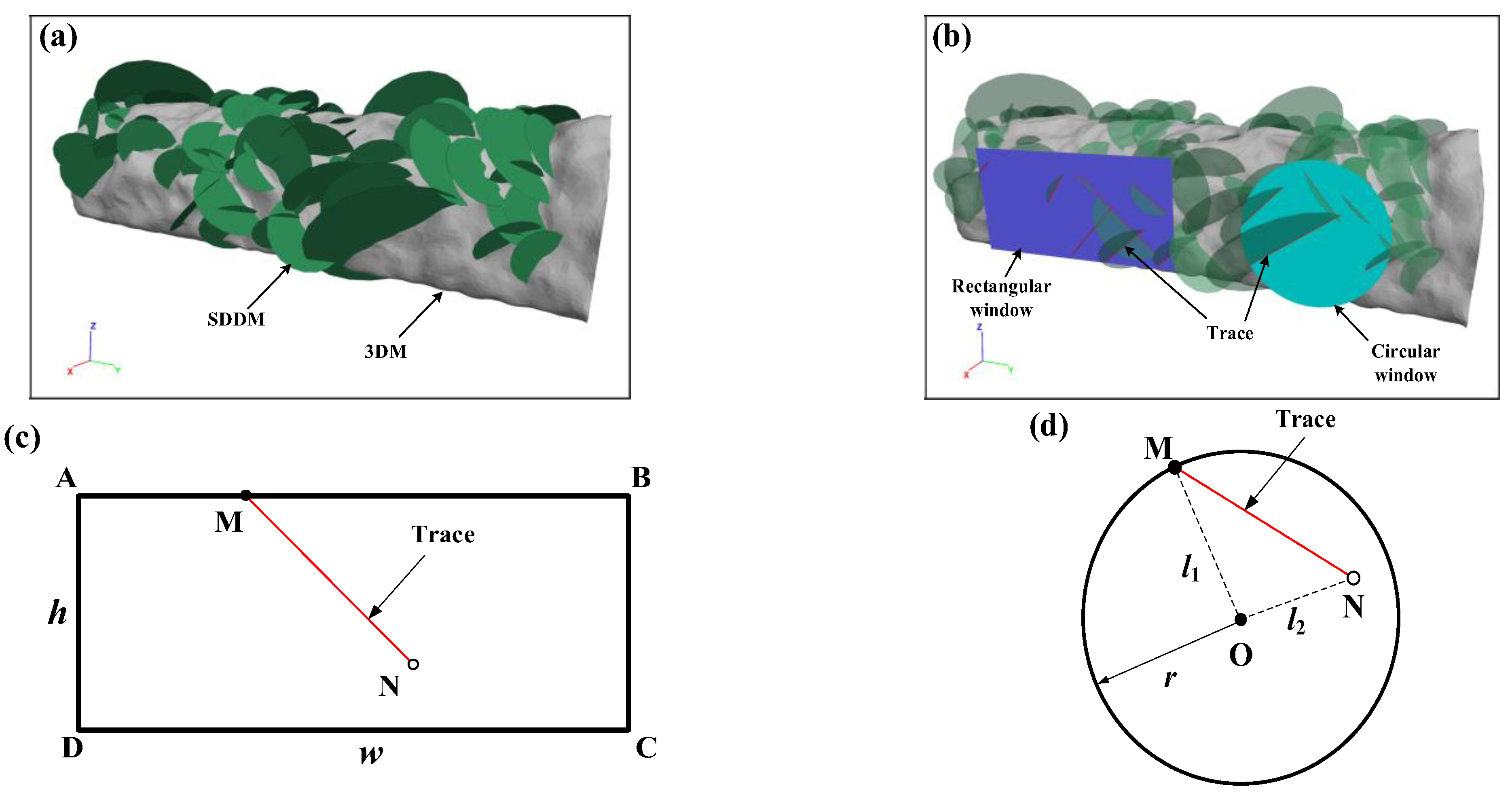
In research, 3DEC [26] is used to set the sampling windows in the 3DM and estimate the mean trace length. The term 3DEC stands for “3D distinct element“; it can import 3DMs and SDDMs (Figure 4a) and achieve a great interaction with PointStudio. In addition, the rectangular and circular sampling windows are set in the 3DM using the geometry generation function of 3DEC; then, the intersection between the SDDM and the sampling window (Figure 4b) can be calculated. Meanwhile, the statistical analysis of the mean trace length can be performed using the FISH program language in 3DEC. Since the SDDM is a simulation of a discontinuity in the field, only the intersection between the discontinuity and the sampling window can be revealed. Therefore, in this study, the positions of the two endpoints of the intersection were used to classify the SDDM located in the sampling window.
In the rectangular sampling window (Figure 4c), if the coordinates of the four vertices A, B, C and D are known, then the spatial linear equations of lAB, lBC, lCD and lode can be obtained. Additionally, coordinates (XM, YM, ZM) and (XN, YN, ZN) of endpoints M and N can be extracted through the FISH program. (1) If the coordinates of M and N both satisfy the linear equations, then the trace intersects the rectangular window; (2) if the coordinates of only one point satisfy the linear equations, it transects the rectangular window; (3) if neither of the two points satisfy the linear equations, it is contained in the rectangular window. Through the statistics of the intersection, mean trace length μ of the structural plane can be estimated with Equation (4).
μ = w h ( 1 + R 0 R 2 ) ( 1 R 0 + R 2 ) ( w E ( sin θ ) + h E ( cos θ ) )
where w and h are the length and width of the rectangular measuring window, respectively; R0 is the ratio of the number of traces intersecting the rectangular window; R2 is the ratio of the number of traces contained in the rectangular window; and θ is the apparent inclination angle of the trace in the direction of the measuring window. In addition, the calculations of E(sinθ) and E(cosθ) of the simplified form consider the orientation biases (more details can be found in Wu et al., 2011 [27]).
Similarly, for a circular sampling window (Figure 3d), coordinates (X, Y, Z) of center O and radius r can be obtained, and lengths l1 and l2 of MO and NO can be calculated. Then, (1) if l1 and l2 are equal to radius r, it is judged that endpoints M and N intersect the circular measuring window, and (2) if l1 and l2 are less than radius r, it is judged that endpoints M and N are contained in the circular sampling window. Through the statistics of the intersection between endpoints M and N, and the circular sampling window, mean trace length μ can be estimated with Equation (5).
μ = π r 2 ( n m )
where m is the number of endpoints contained in the circular sampling window and n is the number of endpoints intersecting the circular measuring window.

4. Sampling Windows Set in 3DM

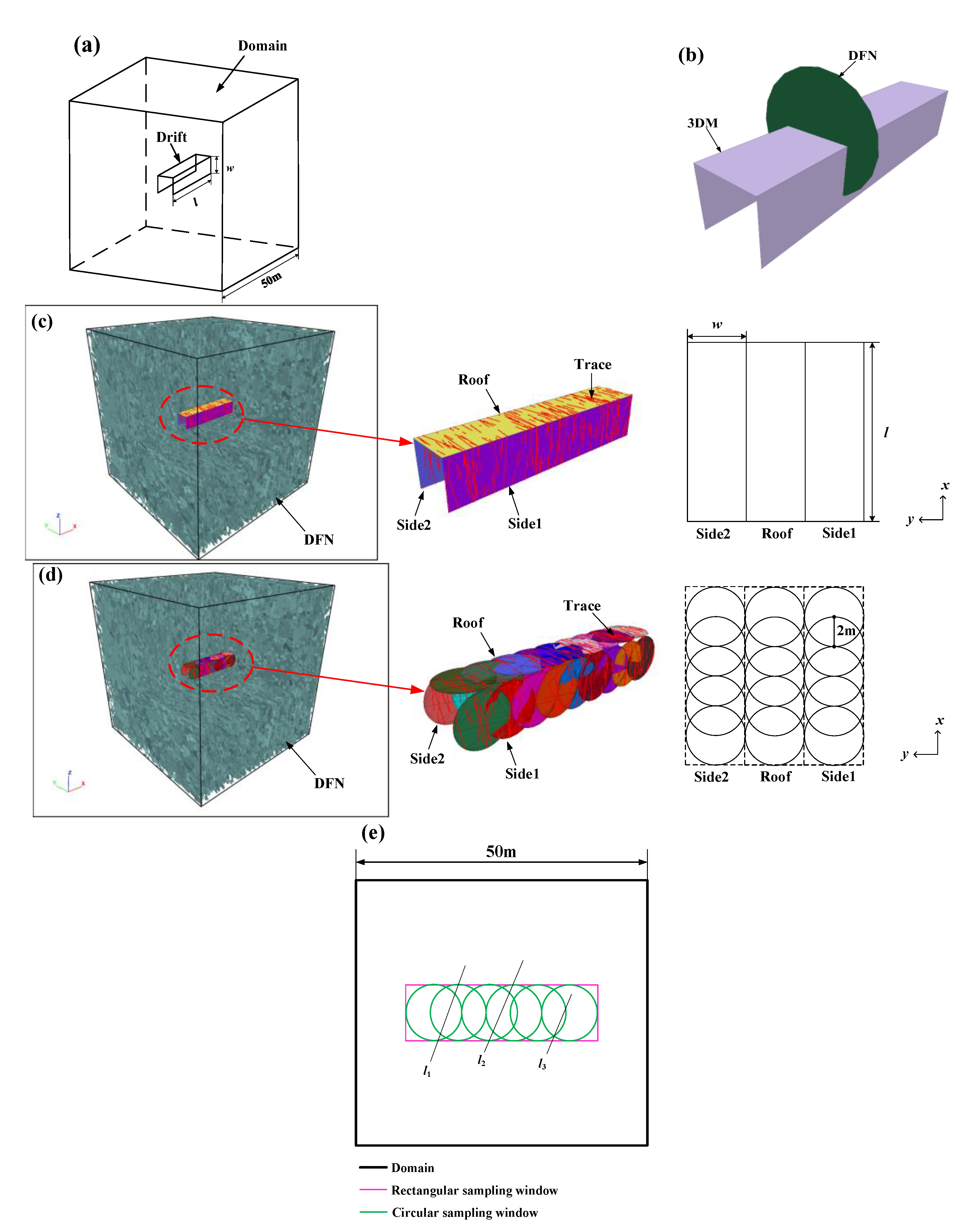
Different from the traditional manual method, the position and number of sampling windows can be arbitrarily set in the 3DM [14], and the roof and sidewalls of the drift can be covered and measured. To better set the sampling windows in the 3DM, we can divide it into a roof area and both side areas, with equal length w and width h; then, the sampling windows are set in these three areas. Due to the difference in the coverage between rectangular and circular sampling windows, their arrangement is also different (Figure 5).
The size of the rectangular sampling window is the same as length w and width h of the area, which can ensure the maximum sampling in this area. However, in the case of the circular sampling window, its size (radius r) is limited by the size of the area width, which cannot cover the entire area directly. Some scholars have discussed the application of circular sampling windows in underground tunnels. For example, Umili [15] conducted sampling by setting multiple concentric circular sampling windows with different radii onto the tunnel face. However, circular sampling windows with different radii can cause sampling deviation, and a reduction in the area of the circular sampling window can lead to an overestimation of the mean trace length. In this study, circular sampling windows with the same radius were set along the long axis of the drift, with an overlapping area between adjacent circular sampling windows. One reason behind this was to ensure that sampling covered the measurement area, and another reason was to ensure the accuracy of repeated sampling. At the same time, to prevent the overlapping area from being too large to cause the same sample value of the two sampling windows, the center distance between adjacent circular sampling windows was taken as radius r.
The mean trace length of each window can be calculated using Equations (4) and (5). Using the averages from Equations (6) and (7), the mean trace length of the rectangular measuring window (μR) and the mean trace length of the circular sampling window (μc) can be obtained.
μ R = ( μ Roof + μ side 1 + μ side 2 ) / 3
μ c = i n μ i t
where μ roof   is the mean trace length of the roof rectangular window; μ side 1 and μ side 2 are the mean trace lengths on both sides, respectively; μ i is the mean trace length of the i-th circular sampling window; and t is the number of circular sampling windows.
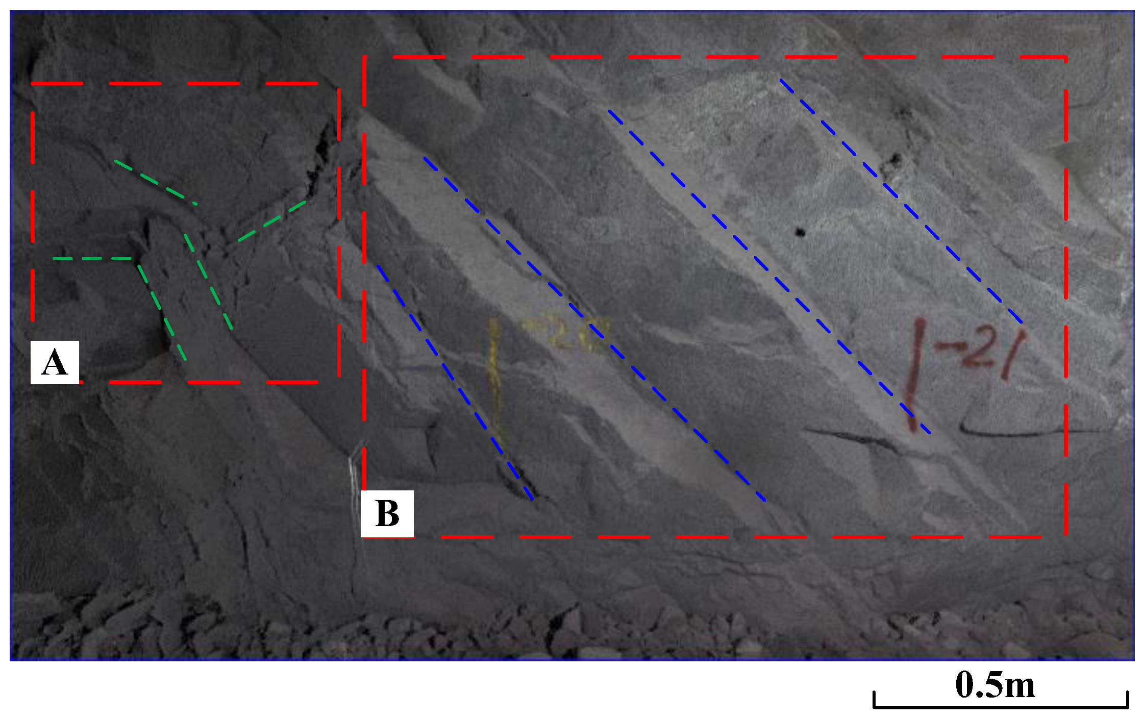
According to the arrangement of the sampling windows in the 3DM, it can be seen that rectangular windows are more convenient and can better cover the sampling area, while circular sampling windows are limited by width h of the measuring area, and overlapping arrangements are required to cover the measurement areas. As the length of the 3DM increases, the advantage of the high coverage of the rectangular window becomes more obvious. However, in our case, the discontinuity was not uniformly exposed in the long and narrow drift. Figure 6 shows that discontinuities with lengths of less than 0.5 m and a relatively concentrated density in area A were mainly developed. Area B mainly showed smooth structural surfaces with a length greater than 2 m with great persistence. This suggests that there are differences in the development of the structural planes of the roadway in the axial or vertical length. If a single measuring window is arranged in this measuring area, sampling errors are more likely to occur. Therefore, to make the estimated value of the average trace length more reliable and ensure the advantages of the circular sampling window for multisampling estimation, the multisampling estimation method needs to be adopted.

5. Comparison of the Two Sampling Methods on the Simulated Case

Wu [27] et al. compared and analyzed the mean trace length of rectangular and circular sampling windows on a rock slope and found that the results of the rectangular sampling windows were more accurate. However, the layout of the sampling windows in the underground drift was different from that of the slope, and there were limitations to sampling in the drift.

5.1. Simulated Case

A simulated case was constructed to compare the statistical results of the two sampling methods using a 3DM, and the numerical model constructed using 3DEC is shown in Figure 7. In the numerical model, a 50 m × 50 m × 50 m cube area was constructed (Figure 7a), and discrete fracture networks (DFNs) were generated with a 100,000-disk discontinuity model in which the center position and diameter were uniformly distributed in space. To avoid the edge effect and study the sampling accuracy of the two sampling methods using 3DMs of different lengths, a 3DM with lengths l of 10 m, 20 m and 30 m and a height w of 4 m was set in the center of the cube as the sampling research object.
The orientation of the discontinuity influences the probability of intersecting the exposed rock face. Even if the rectangular sampling window undergoes probability correction of the orientation of the discontinuity, when the direction is relatively parallel to the exposed rock face, the number of samples of the discontinuities is reduced, which makes the sampling results unreliable. To better analyze the applicability of the two sampling methods using a 3DM, it was assumed that the sampling planes were perpendicular to the DFN (Figure 7b) to reduce the influence of the discontinuity orientation. At the same time, to show the difference in the development of discontinuities in reality, the orientation of DFN conformed to the Fisher distribution of k = 100.
In the simulated case, the two sampling methods were set in the 3DM (Figure 7c,d). The error ratio between the mean trace length obtained using sampling windows and the true trace length ( μ l ) could, therefore, be calculated (Equations (8) and (9)).
ε R = | μ R μ l | μ l × 100 %
ε c = | μ c μ l | μ l × 100 %
where ε R is the error ratio obtained using the rectangular sampling window and ε c is the error ratio obtained using the circular sampling window. True trace length μ l can be easily obtained using 3DEC software using the arithmetic average of lengths l1, l2 and l3 (Figure 7e).

5.2. Results

Based on the simulated model, 100 DFN random generations and sampling estimations were performed (Table 1). For the sampling estimation results of the 3DM of different lengths, the average sampling error of the circular measuring window was approximately 10%, which was smaller than the average sampling error of the rectangular measuring window (approximately 20%). Meanwhile, as the length increased, the average relative error of the estimated value obtained using the rectangular sampling window increased. The main reason may be that the greater the length of a 3DM is, the greater the difference in the development of discontinuities is. Therefore, we can conclude that compared to the rectangular measuring window, the multiple sampling estimation method of the circular sampling window can reduce the sampling error.
Furthermore, to study the influence of the discontinuity density, the number of DFNs generated in the area was increased to 200,000 and 300,000 in the model with a 20 m length 3DM, with 100 random generations and samplings being performed (Table 2). It can be seen that when the number of DFNs increased, the average relative error of the two window measuring methods was reduced (the average relative error of the rectangular sampling window was reduced by 0.24%, and that of the circular sampling window was reduced by 2.11%). The results showed that the increase in the number of samples improved the accuracy of the sampling estimation results, which reflects the importance of the number of samples. Hence, 3D laser scanning point cloud data can obtain a larger number of discontinuity data, which can result in more accurate mean trace length estimation results.
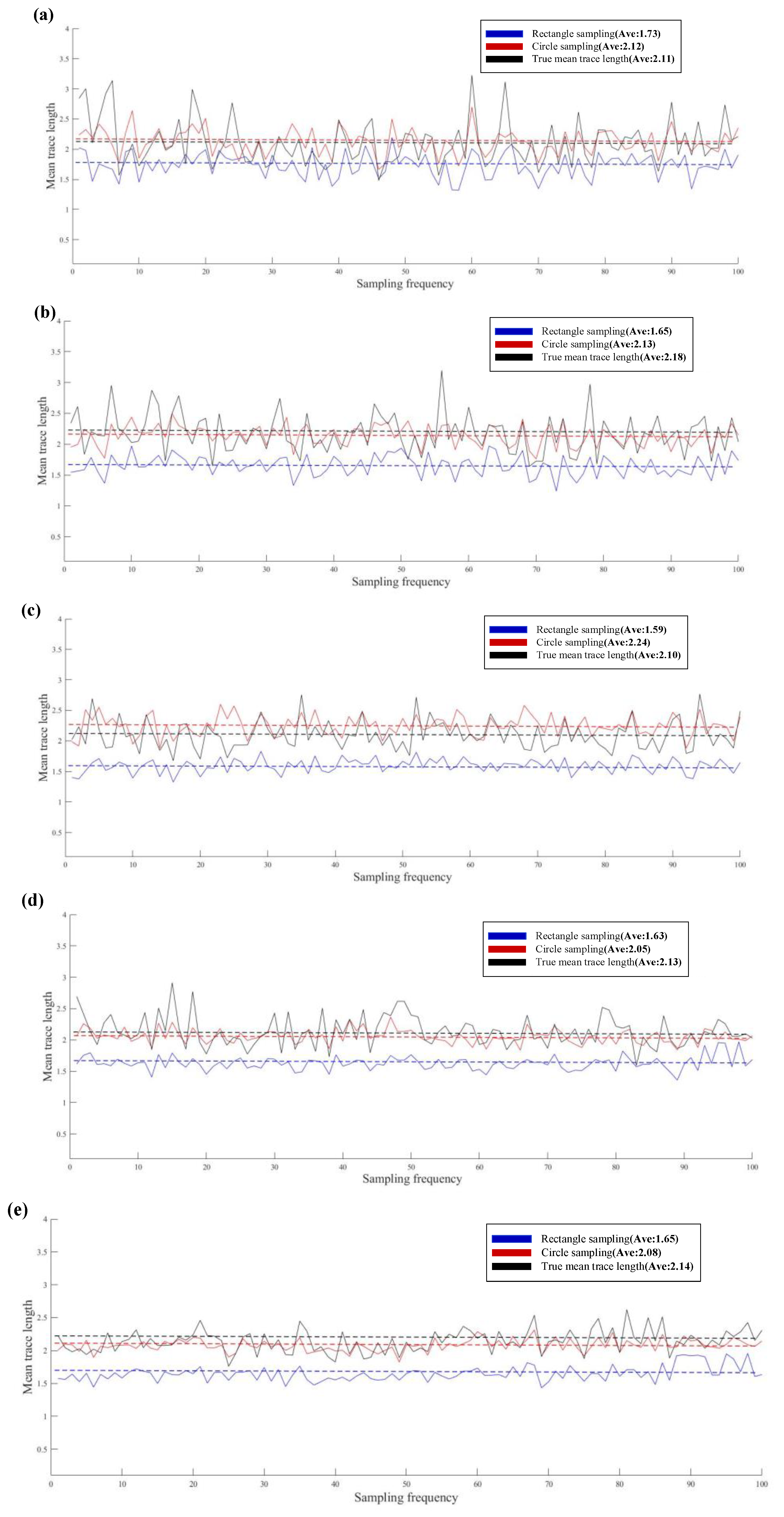
In all simulated cases, it could be determined that the mean trace length estimated using the circular sampling window was closer to the true trace length (Figure 8). Due to the limited exposure conditions, the mean trace length estimated using the rectangular sampling window was always less than the true trace length, but the circular measuring window was overestimated (Figure 8a,c). The main reason may be that the area of the circular sampling window is limited by the height of the 3DM, and it is easy to produce estimates that are larger than the true trace length.
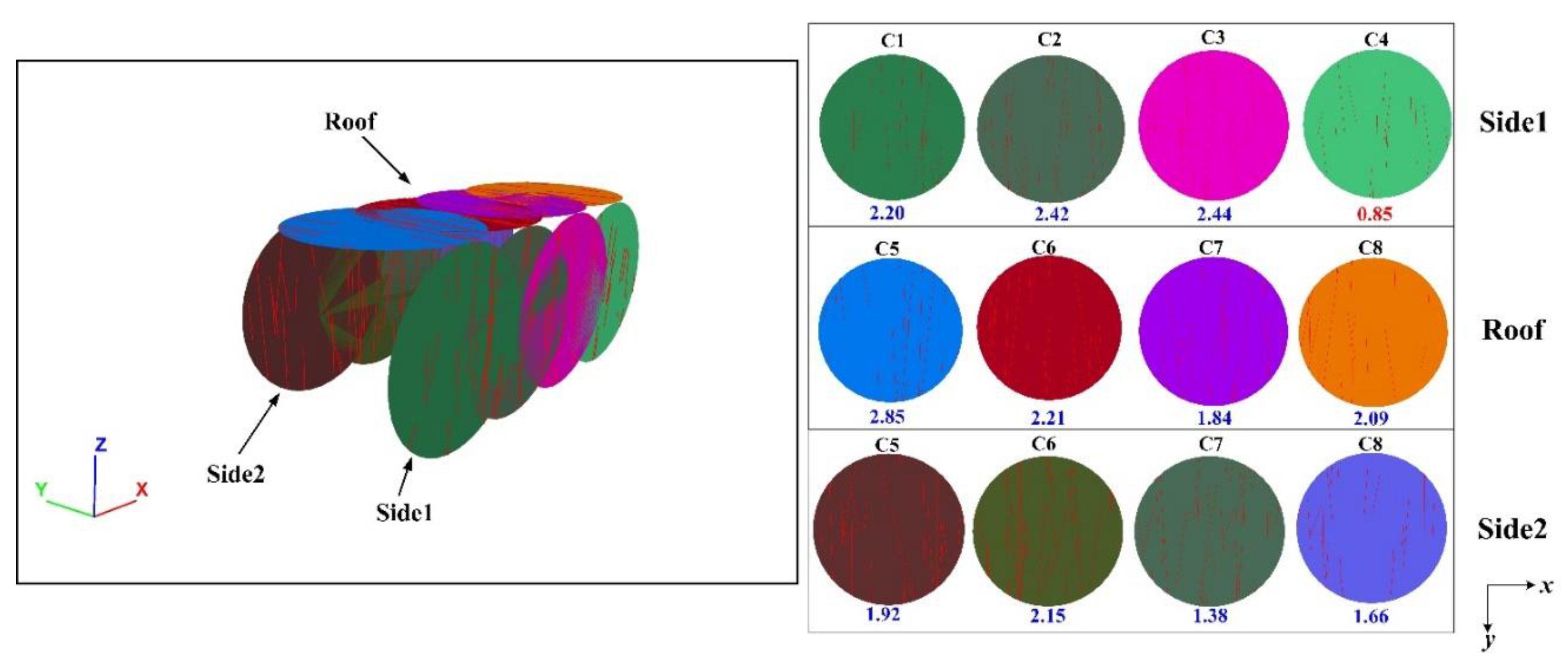
Due to the outcropping restriction of the surrounding rock, the circular window was easier to remove from the outliers. When the length of the 3DM was 10 m and the number of discontinuities was 100,000, the statistical results of the circular sampling window obtained using one of the simulated cases (Figure 9) were used for the analysis. In this case, the true trace length was 2.25 m; the estimation of the mean trace length was 2.00 m, and the relative error was calculated to be 11%. However, we found that the estimation obtained using C4 was abnormal (much smaller than the average), and when we removed this value, the estimation of the mean trace length was changed to 2.10 m, and the relative error was reduced to 6%. Therefore, the outliers in the multiple sampling estimation results of the circular window can be removed in order to reduce the estimation error. In summary, in the sampling window arrangement adopted in this research, the circular sampling window could obtain a more accurate estimate of the mean trace length using the 3DM.

6. Case Study

A 3D laser scanning operation was conducted in drift No. 5 at the 1300 m level of Jianshan Underground Mine in Panzhihua, Sichuan, China. The point cloud data of the drift with a length of 40.32 m were obtained, and an area with a high point cloud quality (18.06 m) was selected as the research area. In this case, PointStudio was used to perform discontinuity data extraction (Figure 10), and a total of 326 discontinuities with an orientation of 327°∠60° were extracted.
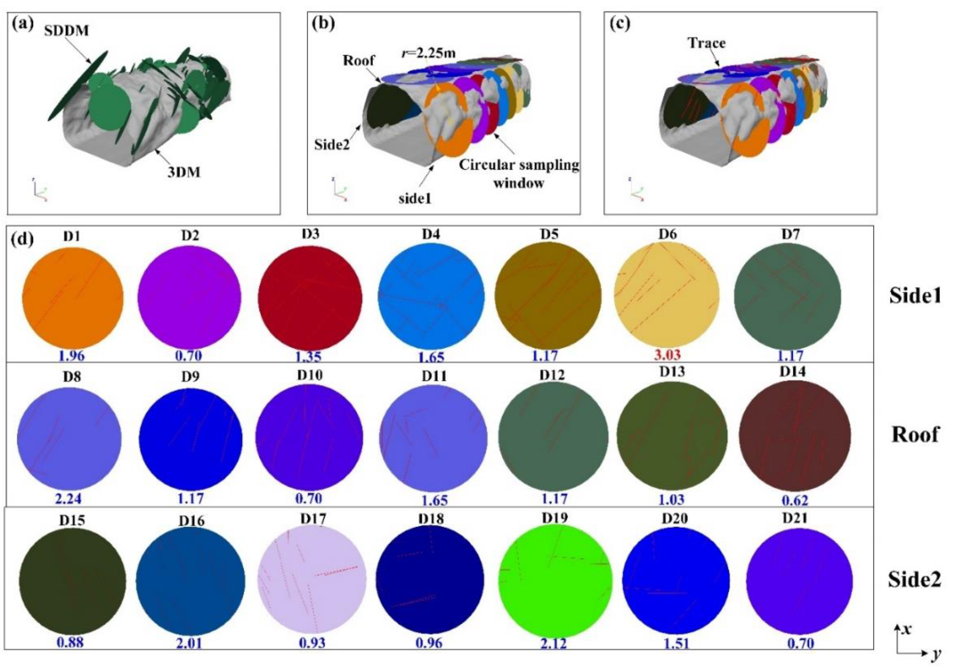
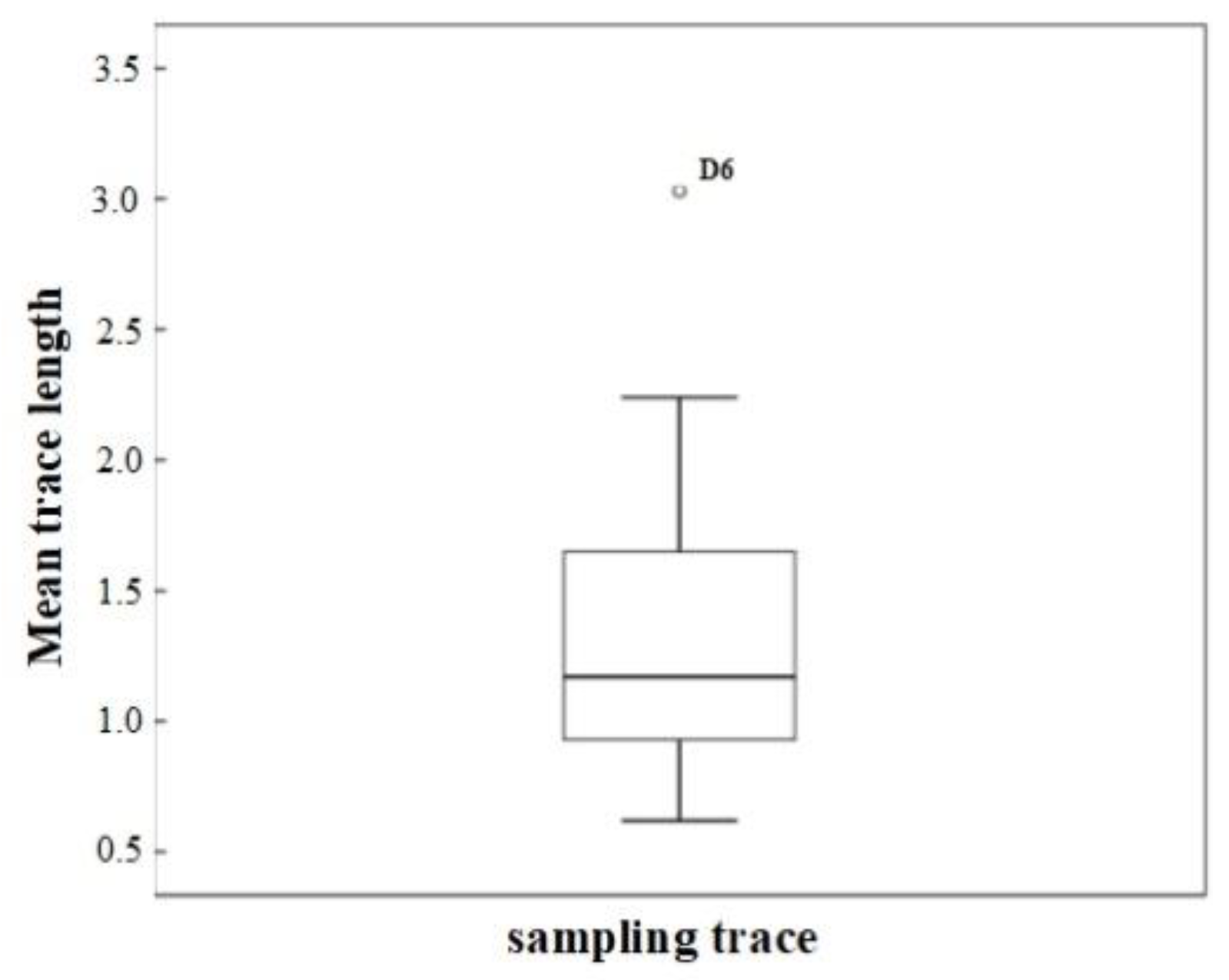
The 3DM constructed with point cloud data and the SDDM extracted in the study area were imported into 3DEC (Figure 11a), and the mean trace length estimation was performed using circular sampling windows. To ensure the coverage of the sampling area, 21 circular sampling windows were arranged on the roof and both sides, in which radius r was set to 2.25 m (Figure 11b). The intersection trace of the SDDM and circular sampling window could be obtained through 3DEC (Figure 11c). Then, the trace sampling result was performed using circular sampling windows D1 to D21 (Figure 11d), and the mean trace length was calculated to be 1.36 m. Then, the boxplot was used to judge the outliers, and it was found that the value estimated using D6 was far from the average value (Figure 12). After the value of D6 was removed, the estimated mean trace length of the research area in drift No. 5 was 1.28 m.
In the engineering field, due to the influence of multiple stages of geological movement, the shape and scale of discontinuities have undergone major changes, and their development has become more discrete. In the partial circular sampling windows (D6 and D8), the discontinuity was well developed, and the mean trace length was relatively large. In addition, discontinuity development in some areas was non-persistent, and the mean trace length obtained was smaller (D2, D9, D14 and D21). Therefore, to conduct better field investigation and sampling, it is necessary to select the exposed position of discontinuities with the best appearance.

7. Conclusions

In this study, a method for analyzing the mean trace length of a discontinuity based on 3D laser scanning was proposed, and the statistical errors of the two different sampling window methods in the drift were compared using 3DEC. The following conclusions can be drawn based on the obtained results:
  • Based on the drift point cloud data obtained using 3D laser scanning, the discontinuities in the drift were extracted, and the virtual sampling windows were laid out in the 3DM using 3DEC software. Then, a method to analyze the mean trace length using the 3DM was proposed.
  • The 3DM was divided into three areas: the roof and both sides. According to the principle of the best area coverage and the largest sampling window size, the size of the rectangular sampling window was arranged according to the area size, and circular sampling windows were continuously arranged with an interval of radius r. Using 3DEC, the mean trace length estimation results of two different sampling windows in the 3DM were compared and analyzed. The results showed that the error value of the mean trace length obtained using the circular measurement window was smaller, and its estimated result was closer to the true value of the trace length.
  • Using the mean trace length estimation method proposed in the study, the mean trace length of a discontinuity was estimated in the selected area of drift No. 5 at the 1300 m level of Jianshan Underground Mine in Panzhihua, Sichuan, China. The results indicated that the mean trace length in the study area was 1.28 m.
  • In this study, 3DEC software was utilized to estimate the mean trace length using a 3DM. In subsequent research, this software can also be used for DFN generation, block instability analyses, and rock support analyses. Moreover, the mean trace length estimation method used in this research can provide an effective basic data extraction method for follow-up research.

Author Contributions

Conceptualization, C.Y. and J.L.; methodology, C.Y..; software, Y.X.; validation, Y.L.; formal analysis, C.Y.; investigation, J.L.; resources, G.S.; data curation, C.Y.; writing—original draft preparation, Y.X.; writing—review and editing, C.Y.; supervision, K.Z.; project administration, J.L.; funding acquisition, J.L. and G.S. All authors have read and agreed to the published version of the manuscript.

Funding

The research presented in this paper was jointly supported by the open project of State Key Laboratory of Safety and Health for Metal Mines “Research on the Automatic Identification Method of the Structural Surfaces and Dangerous Blocks of the Surrounding Rock of Deep High-stress Drift” (grant No. 2020-JSKSSYS-06), the “13th Five-Year” national Key Research and development program “Precision and continuous mining technology and demonstration of boromagite for solid waste source reduction” (grant No. 2020YFC1909801) and the National Natural Science Foundation of China program “Research on dynamic mechanical properties and damage mechanism of rock under the coupling action of freeze-thaw cycle and chemical corrosion” (grant No. 52104109).

Institutional Review Board Statement

Not applicable.

Informed Consent Statement

Not applicable.

Data Availability Statement

Not applicable.

Conflicts of Interest

The authors declare no conflict of interest.

References

  1. Kong, D.; Saroglou, C.; Wu, F.; Sha, P.; Li, B. Development and application of UAV-SfM photogrammetry for quantitative characterization of rock mass discontinuities. Int. J. Rock Mech. Min. Sci. 2021, 141, 104729. [Google Scholar] [CrossRef]
  2. Singh, S.K.; Raval, S.; Banerjee, B.P. Automated structural discontinuity mapping in a rock face occluded by vegetation using mobile laser scanning. Eng. Geol. 2021, 285, 169–175. [Google Scholar] [CrossRef]
  3. Zheng, J.; Deng, J.; Yang, X.; Wei, J.; Zheng, H.; Cui, Y. An improved Monte Carlo simulation method for discontinuity orientations based on Fisher distribution and its program implementation. Comput. Geotech. 2014, 61, 266–276. [Google Scholar] [CrossRef]
  4. ISRM. Suggested methods for the quantitative description of discontinuities in rock masses. Int. J. Rock Mech. Min. Sci. Geomech. Abstr. 1978, 15, 319–368. [Google Scholar] [CrossRef]
  5. Chen, S.; Walske, M.L.; Davies, I.J. Rapid mapping and analysing rock mass discontinuities with 3D terrestrial laser scanning in the underground excavation. Int. J. Rock Mech. Min. Sci. 2018, 110, 28–35. [Google Scholar] [CrossRef]
  6. Fekete, S.; Diederichs, M. Integration of three-dimensional laser scanning with discontinuum modelling for stability analysis of tunnels in blocky rockmasses. Int. J. Rock Mech. Min. Sci. 2013, 57, 11–23. [Google Scholar] [CrossRef]
  7. Havaej, M.; Coggan, J.; Stead, D.; Elmo, D. A Combined Remote Sensing–Numerical Modelling Approach to the Stability Analysis of Delabole Slate Quarry, Cornwall, UK. Rock Mech. Rock Eng. 2015, 49, 1227–1245. [Google Scholar] [CrossRef] [Green Version]
  8. Xu, W.; Zhang, Y.; Li, X.; Wang, X.; Ma, F.; Zhao, J.; Zhang, Y. Extraction and statistics of discontinuity orientation and trace length from typical fractured rock mass: A case study of the Xinchang underground research laboratory site, China. Eng. Geol. 2020, 269, 54–69. [Google Scholar] [CrossRef]
  9. Lyman, G.J. Rock fracture mean trace length estimation and confidence interval calculation using maximum likelihood methods. Int. J. Rock Mech. Min. Sci. 2003, 40, 825–832. [Google Scholar] [CrossRef]
  10. Zhang, L.Y.; Ding, X.B. Variance of non-parametric rock fracture mean trace length estimator. Int. J. Rock Mech. Min. Sci. 2010, 47, 1222–1228. [Google Scholar] [CrossRef]
  11. Sturzenegger, M.; Stead, D. Close-range terrestrial digital photogrammetry and terrestrial laser scanning for discontinuity characterization on rock cuts. Eng. Geol. 2009, 106, 163–182. [Google Scholar] [CrossRef]
  12. Sturzenegger, M.; Stead, D. Quantifying discontinuity orientation and persistence on high mountain rock slopes and large landslides using terrestrial remote sensing techniques. Nat. Hazards Earth Syst. Sci. 2009, 9, 267–287. [Google Scholar] [CrossRef]
  13. Sturzenegger, M.; Stead, D.; Elmo, D. Terrestrial remote sensing-based estimation of mean trace length, trace intensity and block size/shape. Eng. Geol. 2011, 119, 96–111. [Google Scholar] [CrossRef]
  14. Wei, X.; Guo, Y.; Cheng, M.; Wei, J.; Zhang, L.; Huo, L.; Hou, Z. Estimation of Fracture Geometry Parameters and Characterization of Rock Mass Structure for the Beishan Area, China. Acta Geol. Sin.-Engl. Ed. 2020, 94, 1381–1392. [Google Scholar] [CrossRef]
  15. Umili, G.; Ferrero, A.; Einstein, H. A new method for automatic discontinuity traces sampling on rock mass 3D model. Comput. Geosci. 2013, 51, 182–192. [Google Scholar] [CrossRef]
  16. Zhang, Q.; Wang, Q.; Chen, J.; Li, Y.; Ruan, Y. Estimation of mean trace length by setting scanlines in rectangular sampling window. Int. J. Rock Mech. Min. Sci. 2016, 84, 74–79. [Google Scholar] [CrossRef]
  17. Cacciari, P.P.; Futai, M.M. Mapping and characterization of rock discontinuities in a tunnel using 3D terrestrial laser scanning. Bull. Eng. Geol. Environ. 2015, 75, 223–237. [Google Scholar] [CrossRef]
  18. Cacciari, P.P.; Futai, M.M. Modeling a Shallow Rock Tunnel Using Terrestrial Laser Scanning and Discrete Fracture Networks. Rock Mech. Rock Eng. 2017, 50, 1217–1242. [Google Scholar] [CrossRef]
  19. Cacciari, P.P.; Futai, M.M. The Influence of Fresh and Weathered Rock Foliation on the Stability of the Monte Seco Tunnel. Rock Mech. Rock Eng. 2020, 54, 537–558. [Google Scholar] [CrossRef]
  20. Battulwar, R.; Zare-Naghadehi, M.; Emami, E.; Sattarvand, J. A state-of-the-art review of automated extraction of rock mass discontinuity characteristics using three-dimensional surface models. J. Rock Mech. Geotech. Eng. 2021, 13, 920–936. [Google Scholar] [CrossRef]
  21. Ge, Y.; Tang, H.; Xia, D.; Wang, L.; Zhao, B.; Teaway, J.W.; Chen, H.; Zhou, T. Automated measurements of discontinuity geometric properties from a 3D-point cloud based on a modified region growing algorithm. Eng. Geol. 2018, 242, 44–54. [Google Scholar] [CrossRef]
  22. Li, X.; Chen, Z.; Chen, J.; Zhu, H. Automatic characterization of rock mass discontinuities using 3D point clouds. Eng. Geol. 2019, 259, 105131. [Google Scholar] [CrossRef]
  23. Monsalve, J.J.; Baggett, J.; Bishop, R.; Ripepi, N. Application of laser scanning for rock mass characterization and discrete fracture network generation in an underground limestone mine. Int. J. Min. Sci. Technol. 2019, 29, 131–137. [Google Scholar] [CrossRef]
  24. Kulatilake, P.H.S.W.; Wu, T.H. The Density of Discontinuity Traces in Sampling Windows. Int. J. Rock Mech. Mtn. Sci. Geomech. Abstr. 1984, 21, 345–347. [Google Scholar] [CrossRef]
  25. Mauldon, M. Estimating Mean Fracture Trace Length and Density from Observations in Convex Windows. Rock Mech. Rock Eng. 1998, 31, 201–216. [Google Scholar] [CrossRef]
  26. Itasca. 3DEC V 7.0, Minneapolis. 2019. Available online: https://www.itascacg.com/software/downloads/3dec-7-00-update (accessed on 22 October 2022).
  27. Wu, Q.; Kulatilake, P.H.S.W.; Tang, H. Comparison of rock discontinuity mean trace length and density estimation methods using discontinuity data from an outcrop in Wenchuan area, China. Comput. Geotech. 2011, 38, 258–268. [Google Scholar] [CrossRef]
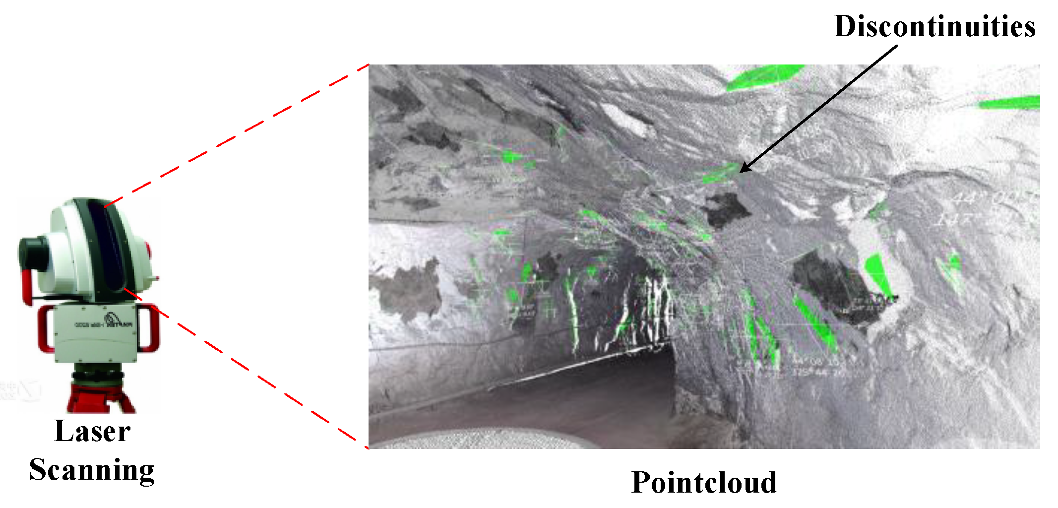
Figure 1. Discontinuity mapping using point cloud data.
Sustainability 14 15650 g001
Figure 2. Structure extraction: (a) discontinuity extraction; (b) diameter and center of SDDM.
Sustainability 14 15650 g002
Figure 3. Method of 3DM construction based on point cloud data.
Sustainability 14 15650 g003
Figure 4. Method of 3DEC model construction and sampling principle: (a) model in 3DEC; (b) sampling window set in 3DEC; (c) rectangular sampling window; (d) circular sampling window.
Sustainability 14 15650 g004
Figure 5. Layout of the sampling window in 3DM.
Sustainability 14 15650 g005
Figure 6. Irregular development of discontinuities.
Sustainability 14 15650 g006
Figure 7. Simulated model: (a) design model (l = 10 m, 20 m and 30 m; w = 4 m); (b) orientation of the DFN; (c) rectangular sampling window (the size of the rectangular window is consistent with the sides and roof of the 3DM); (d) circular sampling window (the radius of the circular window is 2 m, and the relationship between the number of circular windows and length l of the 3DM is l/2-1); (e) true trace length μ l .
Sustainability 14 15650 g007
Figure 8. Comparative analysis results: (a) the number of DFNs was 100,000 for 10 m 3DM; (b) the number of DFNs was 100,000 for 20 m 3DM; (c) the number of DFNs was 100,000 for 30 m 3DM; (d) the number of DFNs was 300,000 for 20 m 3DM; (e) the number of DFNs was 300,000 for 30 m 3DM.
Sustainability 14 15650 g008
Figure 9. Statistical results of the circular sampling window.
Sustainability 14 15650 g009
Figure 10. Point cloud and discontinuities.
Sustainability 14 15650 g010
Figure 11. Mean trace length estimation: (a) importing of SDDM and 3DM in 3DEC; (b) circular sampling window construction; (c) intersection trace with SDDM and sampling window; (d) statistical results of the circular sampling window.
Sustainability 14 15650 g011
Figure 12. Mean trace length estimation.
Sustainability 14 15650 g012
Table 1. Comparative analysis results (100,000 discontinuities).
Drift LengthSampling TimesAverage Relative Error (Rectangular Sampling Window)Average Relative Error (Circular Sampling Window)
10 m10017.49%11.01%
20 m10023.18%9.64%
30 m10023.31%10.65%
Table 2. Comparative analysis results (the length of the roadway was 20 m).
Number of DiscontinuitiesSampling TimesAverage Relative Error (Rectangular Sampling Window)Average Relative Error (Circular Sampling Window)
100,00010023.18%9.64%
200,00010022.99%7.56%
300,00010022.69%5.42%
Publisher’s Note: MDPI stays neutral with regard to jurisdictional claims in published maps and institutional affiliations.