Circular Economy in Winter Road Maintenance: A Simulation Study

Abstract

This study analyzes the sustainability of the circular economy model on winter road maintenance. Winter road maintenance involves plowing snow, spreading abrasives, and then sweeping and collecting the remaining abrasives at the end of the winter season. Traditionally, in the linear approach, the collected sweepings are landfilled, which incurs landfilling costs for resources that could be reused. To address this issue, we consider the option of recycling sweepings for use in the following winter seasons. We develop a discrete-event simulation model that estimates the economic and environmental benefits of this option. Using data from a case study of a highway in Quebec, Canada, the model shows that introducing circular economy practices in winter road maintenance results in less material going to landfills, lower costs, less use of aggregates from virgin materials, and lower CO₂ emissions compared to the linear approach. A subsequent sensitivity analysis reveals that the quantity of sweepings collected greatly influences the outcomes.

1. Introduction

Winter road maintenance, conducted yearly and carried out from November to March, is an essential operation in countries with severe winters, such as Canada, Russia, Sweden, and the USA. Snow is plowed from the roadways to clear them, and abrasives from mineral resources, mainly sand and crushed stones, are spread to provide traction on slippery surfaces. The quantity of abrasives spread each winter is considerable: in Quebec, Canada, one million and fifty-four thousand tons per winter are spread on average only on the 31,000 km road network under the jurisdiction of the Ministère des Transports du Québec [1].

Of the millions of tons spread, a portion is lost, sent off the roads by moving vehicles, water runoff, and the wind. The rest must be removed by mechanical sweeping in the spring. Removing loose abrasives before the summer season improves driving safety and results in less dust raised by vehicles, which reduces environmental and public health hazards.

At present, the collected material is landfilled, as governments have traditionally considered only cost and safety issues and not the environmental impacts of winter road maintenance. Reusing and recycling material collected by spring sweeping represents a potentially sustainable solution to the environmental issues resulting from landfilling. Recent research offers some reuse and recycling alternatives. The prospect of reusing the collected material as an abrasive in winter maintenance has been studied by Donovan [2], Pulley et al. [3], and Mokwa and Foster [4]. Mokhbi et al. [5] proposed using recycled abrasive material as a substitute for raw material in asphalt mixes. However, whereas the idea of collecting and reusing abrasives at the end of the winter season is appealing and has been proven technically feasible, neither the economic feasibility nor the environmental impact has been assessed. One potential drawback is that recycling sweepings involves added processing and transportation requirements, which could increase not only operational costs but also carbon emissions.

Accordingly, this paper aims to analyze the performance of introducing a circular economy strategy by addressing three core questions:

• Will recycling sweepings cost more than landfilling them?
• Will transporting and processing sweepings increase carbon emissions?
• Will enough material be diverted away from the waste stream to justify reusing sweepings in winter road maintenance?

To answer these three questions, we opted for a discrete-event simulation [6,7,8,9]. Discrete-event simulation (DES) is a powerful analytic tool widely applied to model dynamic systems that evolve over time. DES can assess complex systems quickly and cost-effectively without disrupting services, as would happen if tests were run on an existing, operational system. DES also provides the ability to model variability and compare various scenarios. Therefore, it appears to be the right approach for our case.

Using a DES model, we simulate the current linear approach, where all sweepings are landfilled, as well as the alternative approach, where collected materials are diverted away from the waste stream and reused in the same value chain. The quantity of abrasives spread in any given year and the amount collected in spring depend on the weather. Such uncertainty, inherent to winter road maintenance operations, is considered in the model to create a realistic simulation. The model provides estimates of costs, carbon emissions, and material flow under various scenarios.

While considering the specific context of winter road maintenance, we also contribute to the broader subject of sustainability and circular economy. Our study is in line with various studies [10,11,12,13,14] that state that moving from the linear to the circular economy requires a holistic approach that accounts for the different activity costs, reuse options, waste regulations, recovery rates, use of virgin resources, and carbon footprint. Ignoring such factors might jeopardize the development of circular economy initiatives [15].

Applying simulation to assess circular economy initiatives is not new. That said, to the best of our knowledge, the specific context considered in this paper has not been previously addressed. Studies addressing remanufacturing systems are prevalent. Gaspari et al. [16] proposed a simulation framework to support the design and management of such systems. Wakiru et al. [17] applied DES to analyze the effect of remanufacturing on power plant availability and maintenance time. Charnley et al. [18] considered the automotive industry, using system dynamics and discrete-event simulation to evaluate the effect of product quality on inspection, cleaning, and disassembly times. Tsiliyannis [19] proposed a Monte Carlo simulation model to quantify waste monitoring and reduction in cyclic systems in the context of cellular phones. Franco [20] developed a system dynamics simulation model to test the effects of product design and business models on circularity. In the same vein, Moreno et al. [21] designed a DES model to explore the potential of digital intelligence and redistributed manufacturing in implementing circular business models. Recently, Dominguez et al. [22] used multi-agent simulation to investigate how remanufacturing configuration impacts the performance of closed-loop supply chains.

Simulation models have also been used to analyze the economic and environmental benefits of waste valorization. Ye et al. [23] discussed coupling coal and municipal solid waste incineration to generate power, whereas Weber et al. [24] considered converting sweet potato waste into ethanol and distilled alcohol. De Oliveira et al. [25] assessed and compared two alternatives to valorize aseptic carton packages, namely recycling through plasma technology and incineration for energy recovery. The recycling of asphalt pavement has been addressed by Yu et al. [26], who compared two recycling methods: the remixing method and the repaving method. Although the context is close to ours, the objectives of our study are different from theirs. The authors analyzed the benefits of the already-existing practice of recycling pavement from an environmental perspective to identify the most appropriate method. On the other hand, our study simulates an alternative practice that is not yet used. In doing so, we compare a linear to circular approach not only from the environmental perspective but also from the economic perspective, taking into consideration our three research questions. Such analysis can help public authorities adopt circular economy practices as part of normal operations.

The remainder of the paper is organized as follows. In Section 2, we present the research methodology. Simulation results are presented and analyzed in Section 3. Conclusions and future work follow in Section 4.

2. Materials and Methods

In general, a simulation study includes the following main steps [6,7,8,9]:

• Problem analysis and information collection
• Data collection
• Model construction
• Model validation and verification
• Designing and conducting simulation experiments
• Output analysis.

Details about the first four steps are provided in this section. The last two steps are discussed in Section 3. Specifically, Section 2.1 describes the existing linear approach and the alternative circular approach (step 1). In Section 2.2 and Section 2.3, we introduce the case study and present the data inputs and measures used to assess the performance of the two approaches (step 2). Finally, Section 2.4 focuses on the simulation software and the methods used to verify and validate the simulation model (steps 3 and 4).

2.1. Overview of the Linear and Circular Approaches

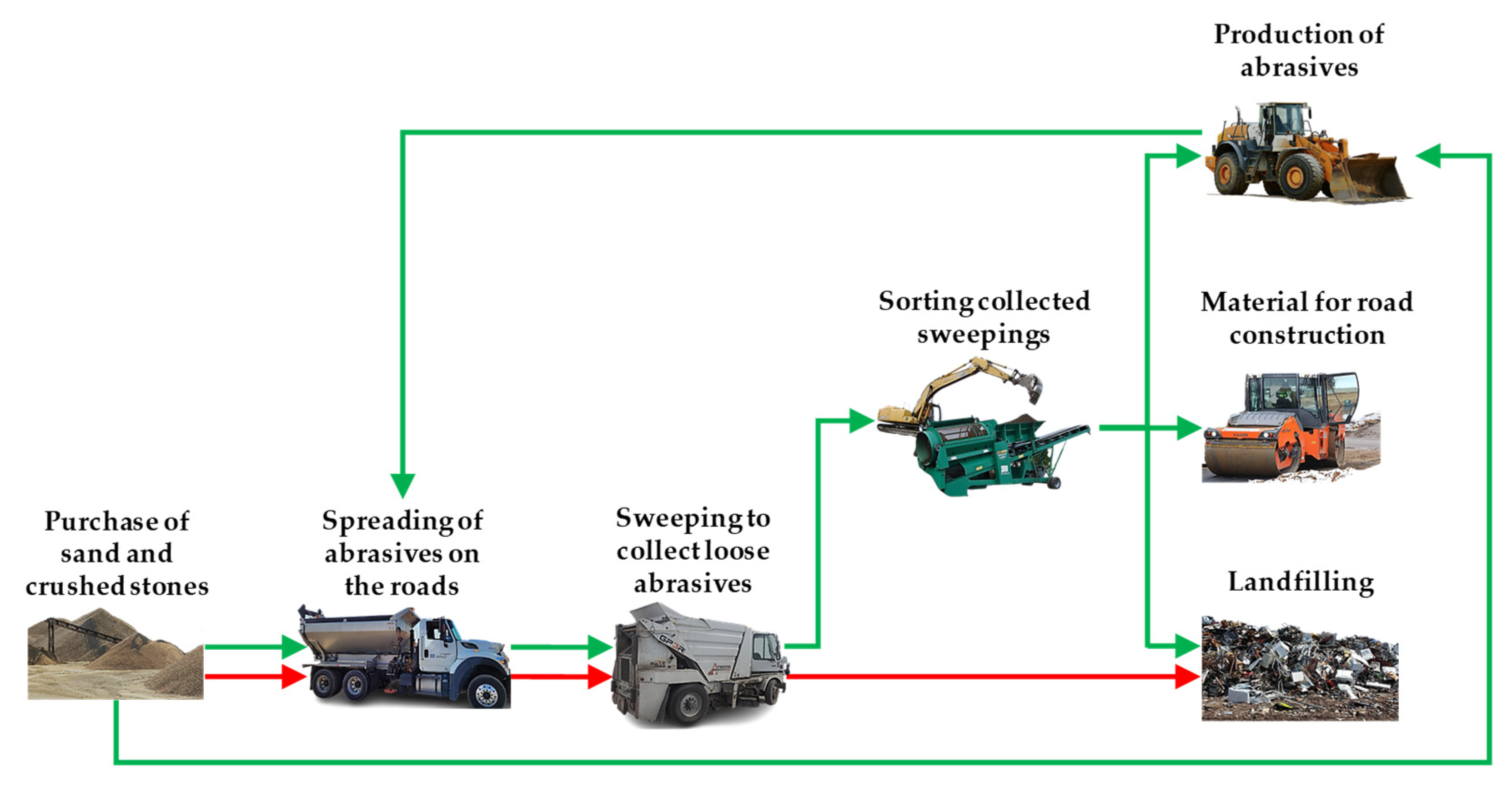
As shown in Figure 1, abrasives spread in winter are made from coarse aggregates (crushed stones) and fine aggregates (sand). These materials are bought from quarries or intermediate vendors and placed in a storage area, where they are blended before being spread on roads. The total amount spread and the ratio of sand to crushed stone in the mixture depends on the severity of the winter, which varies from year to year. At the end of the winter season, abrasives that remain on the roads are collected by road sweepers during spring maintenance. The collected/spread ratio, henceforth referred to as the collection rate, depends on the type of road and the weather conditions.

In the linear approach, all the sweepings are landfilled. The landfilling fees depend on the degree of contamination in the sweepings, which include undesirable materials such as glass, metal, plastic, hydrocarbons, road litter, leaves, grass, and soil, the amounts of which vary from truckload to truckload of swept material.

The circular approach is meant to reduce landfilling by recycling the collected material. In doing so, the physical and chemical properties of the material (e.g., particle size distribution, heavy metal level) must be taken into consideration to comply with engineering and environmental regulations. Collected sweepings are first sieved to separate what can be recycled from what must be landfilled. The material recovered through sifting is thereafter assessed according to specific environmental regulations of the public authority. Only material deemed to be slightly contaminated can be reused. Let ${\alpha }_1$ and ${\alpha }_2$ be the approved threshold values of contamination for abrasive reuse, where ${\alpha }_1<{\alpha }_2$. Material whose degree of contamination is below ${\alpha }_1$ is transformed into abrasive road material by adding virgin sand to it in a quantity that linearly depends on its volume. The production is used to meet the needs for sand in future winters. Material whose degree of contamination is above ${\alpha }_1$ but below ${\alpha }_2$ is reused in road construction. Finally, material whose degree of contamination exceeds ${\alpha }_2$ is landfilled. In what follows, we will call the fraction of sweepings recovered after sifting the recovery rate, the fraction of recovered material that will be recycled as road abrasives the recycling rate, and that which goes to road construction the reuse rate.

2.2. Data Inputs

The data used to inform the simulation model include material flow, distance, cost, and carbon dioxide (CO₂) emissions data. We used case-specific data, as explained in the next sections.

2.2.1. Case Study

Trois-Rivières is the largest city in the Mauricie administrative region of the province of Quebec, Canada. It is a regional center located halfway between Montreal and Quebec City with a population of approximately 140,000 [27]. Our research project was designed to assess the potential of recycling spring sweepings in the Trois-Rivières portion of Highway 40, a provincially maintained highway that connects several populous metropolitan areas across Quebec. This portion is used by residents of the core urban area of Trois-Rivières as well as by people who live in adjacent municipalities and passenger and truck traffic traveling to and from Montreal and Quebec City.

The study was developed in collaboration with stakeholders representing the different professionals involved in winter road maintenance as well as experts in sustainable and environmental technologies, namely the Ministère des Transports du Québec (MTQ), Arseno Balayage, Biopterre, and Innofibre. MTQ is the Quebec government ministry responsible for transport, infrastructure, and law in Quebec, including maintenance of provincial highways, roads, and bridges. Arseno Balayage is a sweeping company that has traditionally won the call for tenders for spring maintenance of the portion of the highway under study. Finally, Biopterre and Innofibre are centers for the transfer of technology that do applied research in the areas of environmental technology and sustainable processing technologies, respectively.

The partners listed above were highly involved in the project. Several group workshops involving all partners were held. In addition, we organized several sub-group workshops, smaller meetings in which participants defined parameters related to their respective domains and expertise. The input from our partners enabled us to gain an adequately informed understanding of the problem as well as to validate each step of the research to ensure that the results were meaningful.

2.2.2. Flow and Distance Data

Table 1. Flow parameters used in the simulation.

Parameter	Value	Source
Total amount spread (ton)	Triangular (5185, 6850, 9309)	MTQ
Proportion of sand in the mix (%)	Triangular (85.50, 90.10, 94.60)	MTQ
Collection rate (%)	Uniform (3.55, 5.59)	MTQ
Recovery rate (%)	Triangular (97.30, 98.10, 99.10)	Innofibre
Recycling rate (%)	44.40	[29]
Reuse rate (%)	53.10	[29]

summarizes the flow data. The total amount spread, the proportion of sand in the mixture, and the collection rate are modeled as stochastic processes to capture the weather dependency of the operations. The distributions used to represent these three input parameters are based on historical data for the years 2015–2020 provided by the MTQ. The collected data were preprocessed and then fitted to probability distributions using the EasyFit software [28].

The recovery rate is also modeled as a stochastic process. Since no historical data is available for this rate, sifting tests were performed by Innofibre using four samples of abrasives collected in 2020 on different types of roads, and the results were used as a surrogate dataset. This dataset was imported to EasyFit for distribution fitting.

Finally, the recycling and reuse rates were taken from Bouchard et al. [29] who analyzed over 100 samples of sweepings characterization data. Note that in Quebec, the reuse and recycling of abrasives are governed by strict regulations [30]. These regulations were considered in estimating the two rates.

Table 2. Distance parameters used in the simulation.

From	To	Distance (km)	Source
Quarry providing sand	Storage area	27.8	MTQ
Quarry providing crushed stones	Storage area	48.1	MTQ
Highway 40	Landfill	20	Arseno
Highway 40	Processing site	12.4	Arseno and MTQ
Processing site	Landfill	19	Arseno and MTQ

summarizes transportation distance data. Distances are given in kilometers and were calculated using Google Maps based on information on the location of the different sites provided by the partners. We assumed, in concert with our partners, that the processing equipment would be placed in the same location as the storage area where virgin abrasives are kept and blended.

2.2.3. Cost and CO₂ Emissions Data

Cost and CO₂ emissions parameters are shown in Table 3. They are defined as constants (deterministic inputs), as their variability is not significant for the scope of this study. However, the proposed simulation model is general and can be tailored to situations where these parameters are stochastic.

The values listed in Table 3 were obtained either from our partners or from the literature. Sand and crushed stone costs were obtained from the MTQ, and the CO₂ emissions resulting from producing these virgin abrasives are from Akan et al. [31]. Arseno Balayage supplied the landfilling costs, whereas information related to transportation costs was obtained from Arseno and the MTQ. CO₂ emissions resulting from transportation were determined using a model that estimates fuel consumption, which depends on the vehicle load and speed [32]. The sorting costs and CO₂ emissions resulting from sorting were provided by Innofibre.

Finally, the proportionality coefficient for winter sand production (i.e., the amount of virgin sand to add to each ton of material recovered from the collected sweepings) was set at 3 in compliance with the norm outlined in [33]. The costs and CO₂ emissions related to this operation were furnished by Innofibre.

Table 3. Cost and CO₂ emissions parameters used in the simulation.

Category	Description	Value	Source
Virgin abrasives	Sand cost ($/ton)	4	MTQ
	Crushed stones cost ($/ton)	21.2	MTQ
	CO2 emissions (kg CO2 eq/ton produced)	5	[31]
Transportation	Cost ($/km)	4	Arseno and MTQ
	CO2 emissions (kg CO2 eq/km)	1.19	Fuel consumption model
Sorting	Cost ($/ton)	1.47	Innofibre
	CO2 emissions (kg CO2 eq/ton)	1.18	Innofibre
Production of abrasives	Proportionality coefficient	3:1	[33]
	Cost ($/ton)	1.19	Innofibre
	CO2 emissions (kg CO2 eq/ton)	0.67	Innofibre
Landfilling	Slightly contaminated material cost ($/ton)	25	Arseno
	Highly contaminated material cost ($/ton)	145	Arseno

Table 3. Cost and CO₂ emissions parameters used in the simulation.

Category	Description	Value	Source
Virgin abrasives	Sand cost ($/ton)	4	MTQ
	Crushed stones cost ($/ton)	21.2	MTQ
	CO2 emissions (kg CO2 eq/ton produced)	5	[31]
Transportation	Cost ($/km)	4	Arseno and MTQ
	CO2 emissions (kg CO2 eq/km)	1.19	Fuel consumption model
Sorting	Cost ($/ton)	1.47	Innofibre
	CO2 emissions (kg CO2 eq/ton)	1.18	Innofibre
Production of abrasives	Proportionality coefficient	3:1	[33]
	Cost ($/ton)	1.19	Innofibre
	CO2 emissions (kg CO2 eq/ton)	0.67	Innofibre
Landfilling	Slightly contaminated material cost ($/ton)	25	Arseno
	Highly contaminated material cost ($/ton)	145	Arseno

2.3. Model Outputs

The primary model output is the total cost per year. The total cost in this study includes the costs to purchase abrasives (sand and crushed stones), transport the abrasives to the storage area, transport the sweepings to landfills, transport the sweepings to processing sites, and process the sweepings (sifting, checking contamination levels, and converting into abrasive road material). Note that the spreading and sweeping costs are not included because they are similar whether the linear or the circular approach is used.

Total CO₂ emissions per year are also a primary concern. In this study, only emissions from the production of virgin abrasives, transportation, and processing operations are considered. Spreading and sweeping emissions are excluded because again, the emissions are the same for the linear and circular models.

Other performance measures are also used to assess the potential environmental benefits of the circular approach. Those measures are related to material flow and include the number of virgin abrasives bought per year, the amount of material landfilled per year, and the quantity of sweepings transformed into abrasive road material.

Details regarding the equations used to calculate the different performance measures are provided in the Appendix A.

2.4. Model Construction, Validation, and Verification

We now present an overview of the methods used in steps 3 and 4 of our simulation study.

2.4.1. Model Construction

The model was built using Simio Simulation Software [34,35]. This software was chosen because it has desirable features, including modeling flexibility (the process approach was used), a good random-number generator, an easy mechanism for making independent replications, built-in animation, and a set of user-friendly features for performing and analyzing simulation experiments. Animation is useful for communicating the model to the stakeholders and accurately debugging and validating it.

2.4.2. Model Validation and Verification

Validation determines to what extent a simulation model can be considered an accurate representation of the real system, whereas verification is employed to ensure that the model is correctly constructed [6,7,8,9].

To validate the model, we adopted the so-called face validation technique [36], which consists of discussing the conceptual model and the simulation results with experts, in our case the stakeholders introduced in Section 2.2.1. The stakeholders agreed that the model is an accurate representation of the system under study. The model was also validated by comparing the total amount of abrasives spread, the proportion of sand in the mixture, and the collection rate to actual data on hand. To this end, ten independent runs of the model were performed. Average estimated values lie, respectively, within 2.27%, 0.56%, and 1.62% difference from average observed values, indicating that the simulation model is a close representation of the actual system.

As for verification, animation was used to ensure that the flow in the simulation model is appropriate and that material is sent to the right destinations. A further verification assessment was undertaken to evaluate the accuracy of the calculation of the performance measures described in Section 2.3. To do so, the model was run with constant input parameters and the simulation outputs were compared to manually calculated results.

3. Results and Discussion

This section describes the last two steps of the simulation study: designing and conducting simulation experiments (Section 3.1) and output analysis (Section 3.2 and Section 3.3). Our findings are summarized in Section 3.4.

3.1. Simulation Runs

We compare the following two scenarios: (i) the linear scenario, where all sweepings are landfilled, which corresponds to the current situation; (ii) the circular scenario, where sweepings would be recycled according to their physical and chemical properties.

Each scenario was simulated 10 times (10 replications), and a different random seed number was used in each run to account for the stochastic nature (variability) of the quantity of abrasives spread each winter, the proportion of sand in the mixture, the collection rate, and the recovery rate. For comparison purposes, the same random numbers have been used in both scenarios. The length of the simulation was set to five years.

3.2. Comparison of the Linear and Circular Scenarios for the Case Study

This section is dedicated to an extensive comparison between the linear and circular scenarios, using data introduced in Section 2.2. Results of additional experiments to evaluate the impact of the collection rate on the outcomes are presented and discussed in Section 3.3.

We assess the performance of the linear and circular scenarios using the measures introduced in Section 2.3. The different performance measures were computed for each replication and each year. We chose to summarize these detailed results in two ways: first, by computing the average of each performance measure over the 10 replications and the 5 years; and second, by computing the average of each component of each measure over the 10 replications for each year. Looking at how each component fits into the equation allows us to perform a more detailed comparative analysis and provides useful information, which we may not see when simply looking at the average results.

3.2.1. Assessment of Material Flow

Figure 2 and Figure 3 compare the linear scenario to the circular scenario in terms of the quantity of abrasives purchased and the destination of the sweepings, respectively.

In year 1, the same quantity of abrasives is bought in both scenarios, as there is no collected material to be recycled. In years 2 to 5, the amount purchased is lower in the circular scenario than in the linear scenario as part of the demand is filled with recycled material. Because crushed stones are not produced through recycling, the quantity of crushed stones purchased is the same in both scenarios (about 676 tons/year). Over the 5 years, 1.81% less sand is purchased in the circular scenario. Considering both types of abrasives, we observe that on average, 7005.36 tons/year are purchased in the linear scenario. This quantity drops to 6890.66 tons/year in the circular scenario, a reduction of 1.64%. Although this difference seems low, it is significant in terms of cost savings and CO₂ emissions reduction.

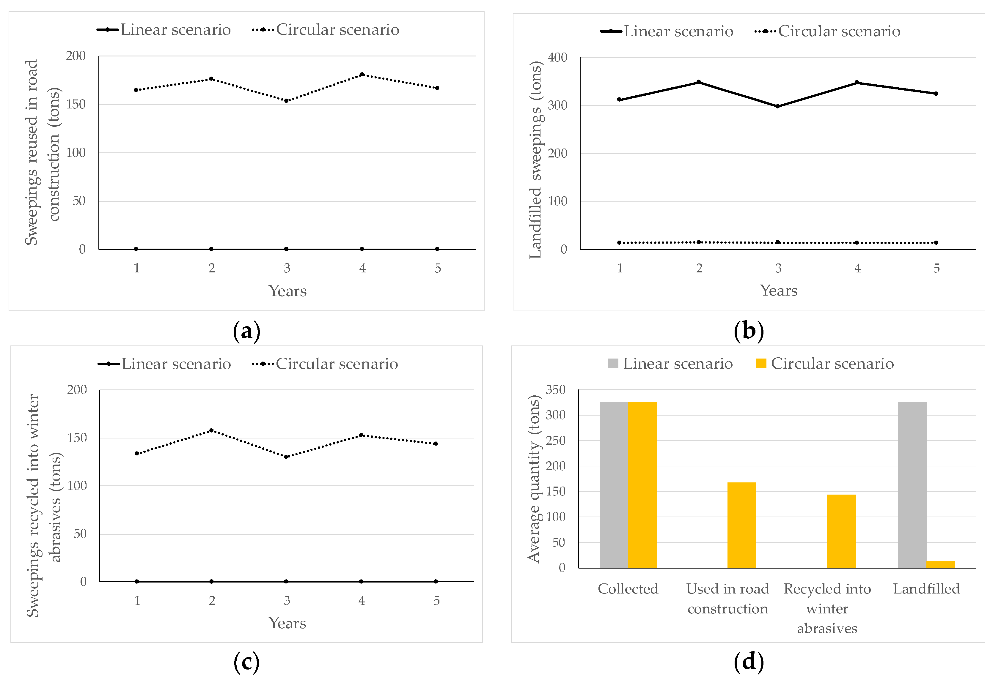
Turning to the destination of the sweepings, Figure 3 shows that the quantity of landfilled sweepings drops drastically in the circular scenario starting in year 1. Each year, more material is diverted for use in road construction than for the production of abrasives, which is expected since the reuse rate is higher than the recycling rate (c.f. Table 1).

All collected sweepings are landfilled in the linear scenario. In contrast, in the circular scenario, on average, of the 325.54 tons of sweepings collected, only 4.25% is landfilled. Of the rest, 51.68% goes to road construction and 44.07% goes to winter abrasives production. This is a significant improvement in terms of land use and money saved on landfilling and on raw materials for both winter road maintenance and road construction.

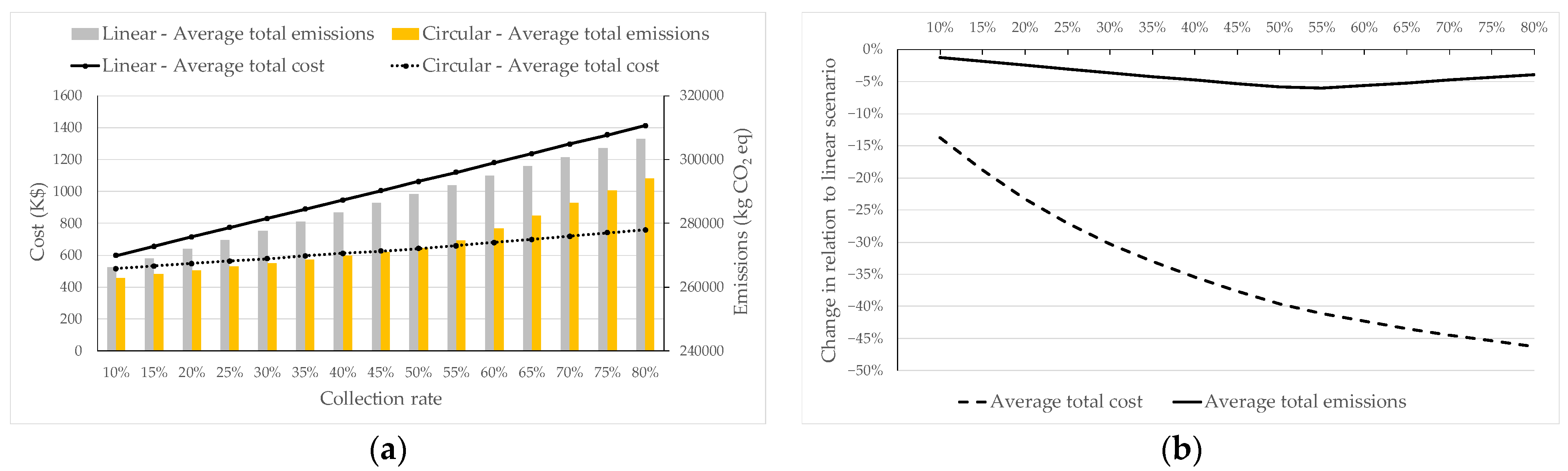
3.2.2. Economic Assessment

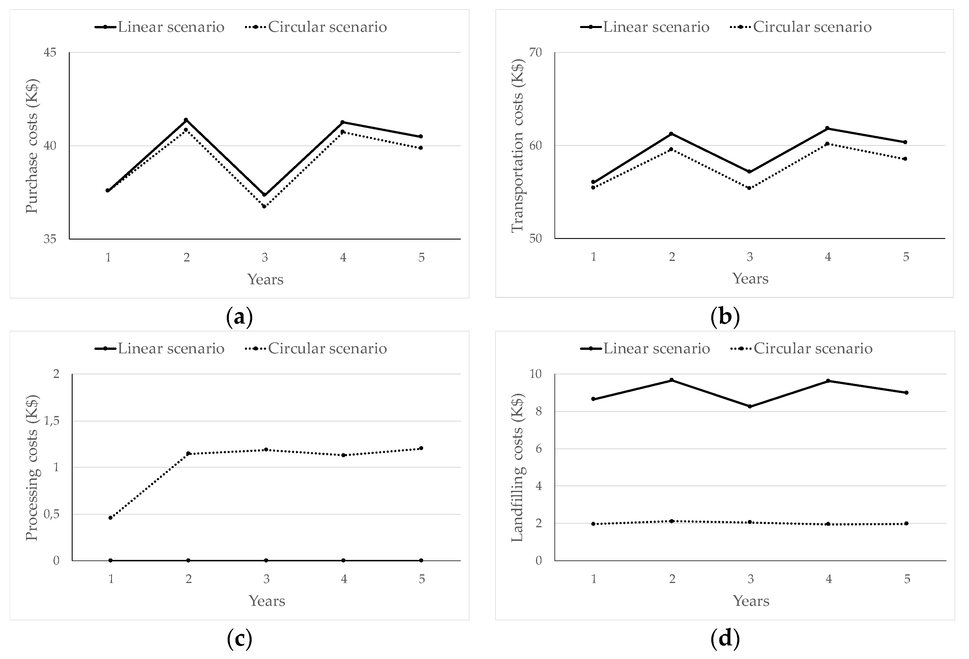
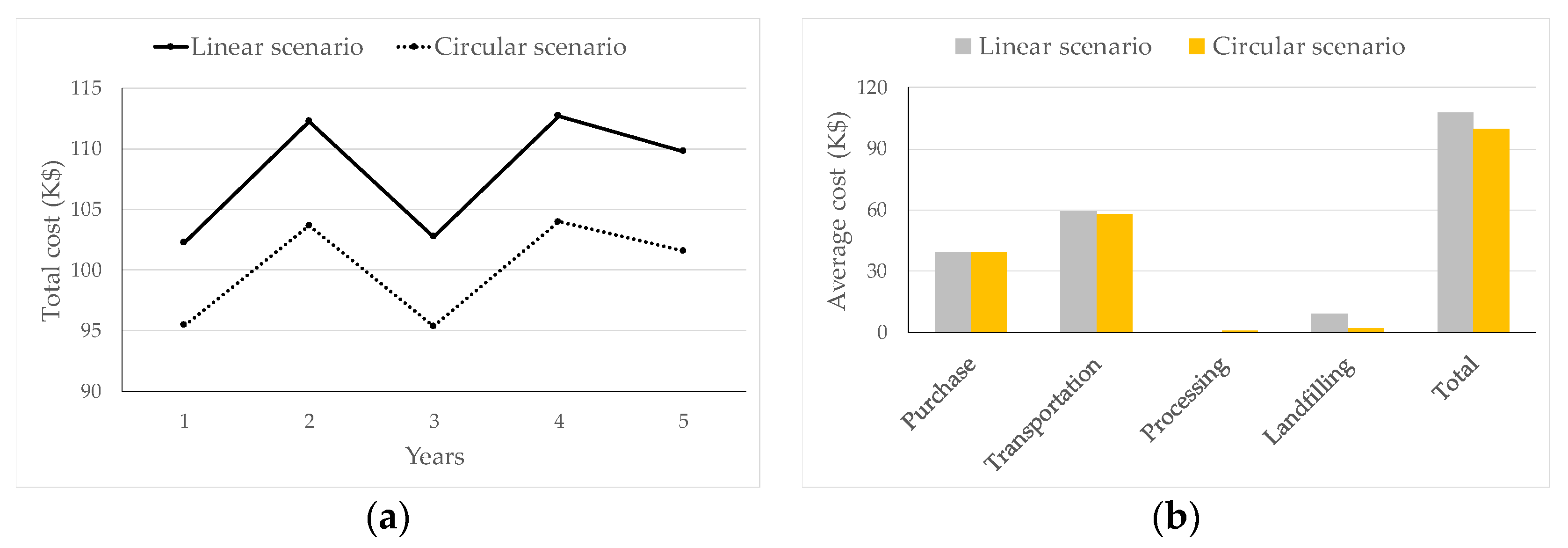
We now compare the two scenarios in terms of costs. Figure 4 shows the values of each cost component per year. A plot of average values over the five years is shown in Figure 5.

Obviously, the purchase costs (Figure 4a) track with the quantity purchased (Figure 2a), and the landfilling costs (Figure 4d) track with the quantity of sweepings landfilled (Figure 3a).

Transportation costs are lower in the circular scenario than in the linear scenario every year (Figure 4b). This might seem counterintuitive, for in the circular scenario there is an extra cost associated with transporting sweepings to processing sites. However, there is a reduction in the costs to transport material to landfills (less quantity means fewer trips) and a reduction in the costs to transport virgin materials to the storage area (less quantity purchased means fewer trips). These savings negate the additional transportation costs incurred by processing.

Finally, it is obvious that processing costs are zero in the linear scenario since all of the collected sweepings are landfilled, whereas they are non-zero in the circular scenario, considering that recovery of sweepings involves additional handling for their sorting and mixing (Figure 4c). We see that they are lower in year 1 because, in that first year, collected sweepings are only sorted to determine what goes where (landfill, road construction, production of abrasives). Starting in year 2, however, there are extra costs incurred by processing the material to produce abrasives to be used in the following years.

In summary, according to our results, on average, the purchase, transportation, and landfilling costs are reduced by 1.16%, 2.51%, and 77.79%, respectively, and the processing costs, which represent only 1.02% of the total cost, increase from $0 to $1024.50, resulting in a net 7.37% reduction in the total cost (Figure 5b).

It is worth noting that although the average reduction in the quantity landfilled is 95.75%, the reduction in the corresponding costs is 77.79%. This is because the landfilling fees depend on the degree of contamination in the sweepings, as already mentioned in Section 2.1 and as can be seen in Table 3. In the linear case, some truckloads of sweepings are less contaminated than others, whereas in the circular case, all material sent to the landfills is highly contaminated and thus more expensive to landfill. Recovered material that is only slightly or moderately contaminated is recycled into winter abrasives or reused in road construction.

3.2.3. Environmental Assessment

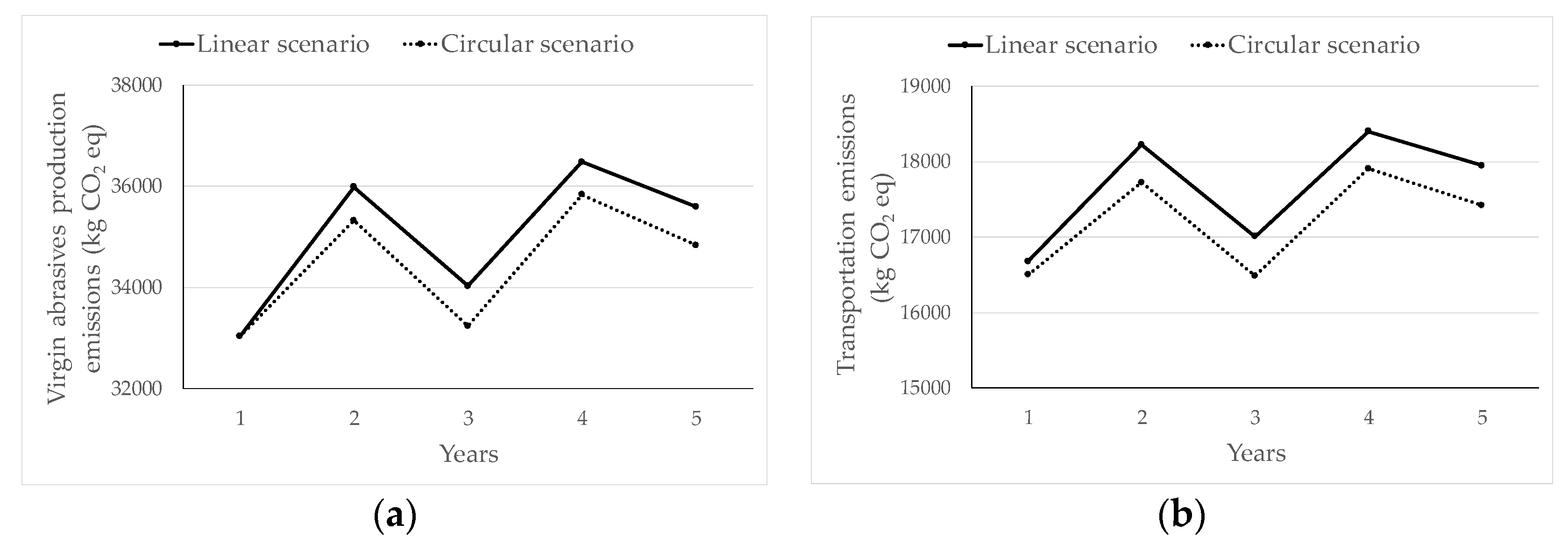
We focus now on carbon emissions (Figure 6 and Figure 7). Just as purchase costs track with the quantity of virgin abrasives purchased, CO₂ emissions resulting from virgin abrasives production track with that quantity. Similarly, the transportation emissions track with the kilometers required to transport all materials, as do transportation costs. Processing emissions depend on the quantity processed as do processing costs. It is thus not surprising that Figure 6a–c look the same as Figure 4a–c, respectively.

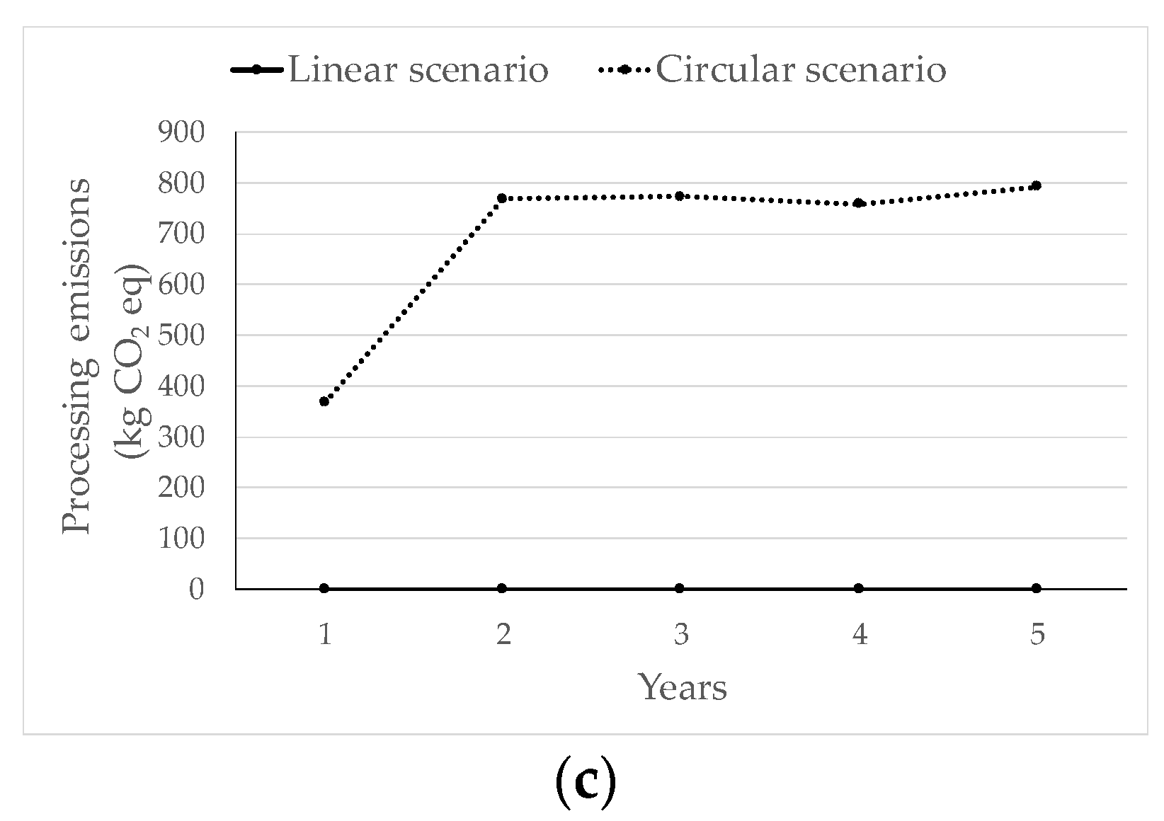
Although there is a reduction in CO₂ emissions in the circular scenario, it is much less impressive than the reduction in costs. In year 1, there is a 0.39% increase in total emissions in the circular scenario (Figure 7a). However, in the following years, total emissions decrease by 0.85% per year on average. Taking the five years together, there is a slight reduction of 0.62% in total emissions in the circular scenario compared to the linear scenario (Figure 7b).

To go into more detail, the largest reduction is obtained in transportation, for which emissions are reduced by 2.51% per year (because fewer trips to landfills and quarries are required, as explained in the previous section). Emissions related to the production of virgin abrasives are reduced by 1.64%. There are clearly extra emissions arising from processing, but they represent only 1.32% of the total emissions and are thus not significant, as can be seen in Figure 7b.

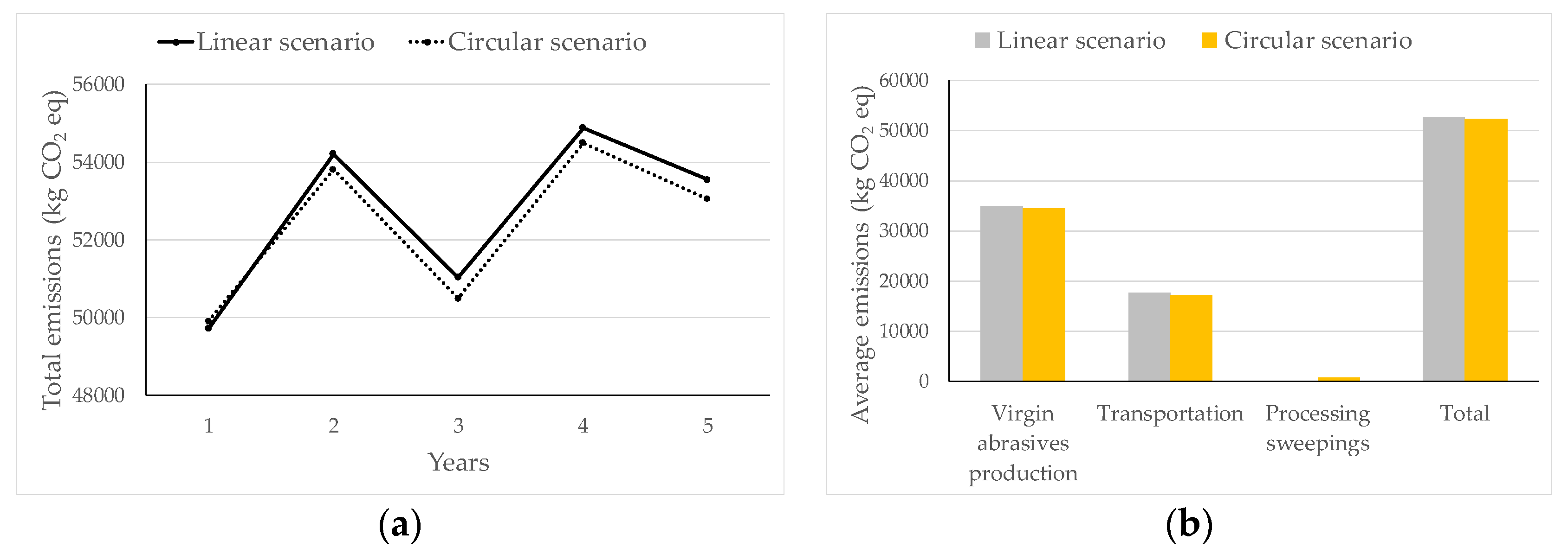
3.3. Effect of Collection Rate

Recall that the collection rate is the percentage of spread material that is collected by sweeping operations in the spring. In the results discussed in Section 3.2, the collection rate for the highway under study is 4.57% on average (c.f. Table 1). Collection rates for municipal roads and streets are higher than collection rates for highways, going as high as 80% [2]. Theoretically, more gains may be obtained if the collection rate is higher. To see what the gains might be, we simulated a range of collection rates from 10% to 80% without altering the values of the other parameters. We focused on two performance measures: total cost and total CO₂ emissions. 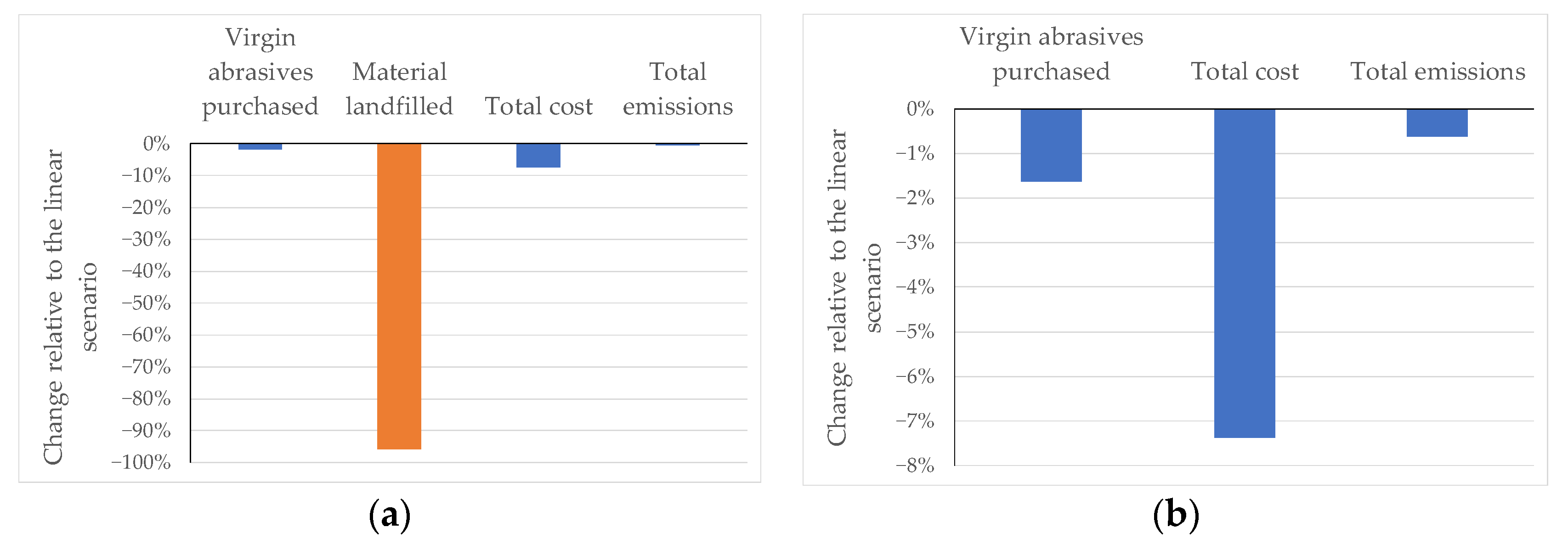Figure 8a shows the average results obtained (average over the 10 replications and 5 years), and Figure 8b illustrates the changes relative to the linear scenario. These changes are the percentage difference between the average total cost (average total emissions) in the linear scenario and the circular scenario. They were calculated using the following equations:

$$\mathsf{\Delta }C=\frac{C^c-C^l}{C^l}\times 100$$

(1)

$$\mathsf{\Delta }E=\frac{E^c-E^l}{E^l}\times 100$$

(2)

where $C^c, C^l$, $E^c$, and $E^l$ are the average total cost in the circular scenario, the average total cost in the linear scenario, the average total emissions in the circular scenario, and the average total emissions in the linear scenario, respectively.

Not so surprisingly, we found that a significant cost saving is possible relative to the linear case. Recall that when the average collection rate was 4.75%, the reduction in total cost was 7.37%. When this rate increases to 10%, the total cost is reduced by 13.77%. This reduction reaches 46.21% when the collection rate is 80%. What was surprising is that the rate at which the cost is reduced decreases as the collection rate increases above 50%.

The reduction in CO₂ emissions doubles when the average collection rate moves from 4.97% to 10% (average reduction moves from 0.62% to 1.26%). The reduction reaches a peak of 5.98% when the collection rate is 55%. From that point on, the reduction decreases gradually until 3.98%, at a collection rate of 80%.

In sum, the total cost keeps decreasing when the collection rate increases, but at a rate that gradually decelerates (more significant decreases are obtained when the increase in collection rate is smaller than 55%). Similarly, emissions also decrease, but the savings start to become lower once the collection rate reaches 55%. This behavior can be explained by the fact that there is a surplus in material that could be used as abrasives when the collection rate is high; that is, an amount left over after the demand is satisfied. Figure 9 provides the average surplus over the 10 replications for each of the first four years. Year 5 is excluded from the analysis because we don’t know what the demand for abrasives will be in year 6, this year not being considered in the study, as it falls outside the planning horizon.

Let’s consider year 1. It can be observed that, whatever the collection rate is, there is no surplus from year 1. All the sweepings recovered in that year that could be used in winter maintenance are used in the following year. This is not the case for years 2 to 4, except when the collection rate is below 50%. When the collection rate is 55%, there is a surplus from year 3 that cannot be absorbed by the next season’s demand. As the collection rate reaches 60%, the material recovered each year that could be used as abrasives exceed the demand for the next seasons. Collecting more material entails more trips to various destinations, which leads to higher truck mileage, transportation costs, and transportation emissions. Processing more material incurs higher processing costs and produces more emissions. When the material is processed and not used, the increase in processing costs and processing emissions is not offset by the decrease in other costs and emissions as much as it is when all material processed is used.

That said, the circular scenario outperforms the linear scenario whatever the collection rate is.

3.4. Summary of the Results

The simulation results allow us to answer our three research questions:

• Will recycling sweepings cost more than landfilling them?
• Will transporting and processing sweepings increase carbon emissions?
• Will enough material be diverted away from the waste stream to justify reusing sweepings in winter road maintenance?

First, based on the results of the case study, recycling sweepings seems to be advantageous with respect to the total cost. A reduction in costs of 7.37% occurs relative to the linear scenario. The savings in landfilling and purchase costs are enough to negate any additional transportation and processing costs. Second, transporting and processing sweepings does not increase carbon emissions. Quite the contrary, CO₂ emissions are reduced, although this reduction is modest, at only 0.62%. In our computations, neither the economic impact nor emissions from material that goes to road construction have been accounted for. If we were to consider that material, the reduction in CO₂ emissions and the economic benefits would probably be higher.

Finally, regarding diverting waste away from the waste stream, the difference between the linear and the circular scenario is quite pronounced: 95.75% less waste is landfilled in the circular scenario. This represents a significant reduction in the quantity of the materials going to landfills and the related costs, both financial and environmental. As can be seen from Figure 10, recycling sweepings also reduces the use of virgin abrasives by 1.64%.

These conclusions are valid for the case study considered in the paper, under the assumption that the collection rate is uniformly distributed between 3.55% and 5.59%. Our analysis of what happens in terms of costs and emissions under higher collection rates indicates that an increase in the collection rate positively affects total costs and total emissions. However, as the collection rate increases, there is a possibility of a surplus of recovered abrasives. This surplus can be sold or used in road construction materials. Logic tells us that the economic impacts and carbon footprint should improve if we consider these options.

It is thus clear from the results presented above that it is worthwhile to integrate circular economy practices into winter road maintenance. Recycling abrasives has the potential to address concerns about landfilling and the depletion of non-renewable resources, and, to a lesser extent, reduce CO₂ emissions. We believe that, though our study concerns a highway in Quebec, the insights obtained can be applied to other regions with similar conditions and concerns.

4. Conclusions

Winter road maintenance uses natural resources, produces waste, and releases GHG emissions, creating a significant impact on the environment. Given this, introducing a circular economy approach in this activity is appealing. Recycled sweepings can be used as a replacement for natural aggregates from virgin materials, in the interests of moving from a waste disposal-oriented system to a life cycle-oriented system, as stated in the literature. However, the economic viability is uncertain. To assess in economic and environmental terms the option of recycling sweepings for winter road maintenance, we developed a discrete-event simulation model. Data related to a case study in Quebec, Canada was used to run the model.

The results show that by recycling sweepings, the authorities in charge of winter road maintenance can reduce their costs and carbon footprint and contribute to the preservation of natural resources. The use of virgin abrasives is reduced by about 2%, thereby decreasing the rate at which natural resources are depleted, and the total cost is reduced by approximately 7%. In terms of environmental benefits, CO₂ emissions are reduced by 0.62%, and landfilling is reduced by approximately 96%, which is a major benefit for land use and the environment. In addition, the results of the sensitivity analysis indicated that an increase in collection rate would result in increased cost savings and lower CO₂ emissions.

Importantly, this study was conducted with the input and validation of stakeholders at every step. The positive indications derived from our research should encourage policymakers to initiate changes in the winter road maintenance system and the associated environmental regulations in order to implement a circular value chain as a step towards a more sustainable society.

Beyond the results of this paper indicating the potential for the development a of viable circular scenario, research issues remain as the detour of sweepings from landfill by their recovery implies the need to update current operating practices in addition to raising the opportunity for infrastructure mutualization between road authorities. Further research is therefore needed to wisely support a fair and sustainable implementation for all stakeholders of the new circular economic model in winter road maintenance.

It should be noted that our simulation model has limitations. First, data is scant, so it was necessary to derive some model parameters from the literature. The lack of data meant that neither the variability of the reuse rate nor the variability of the recycling rate could be considered. The gain from material reused in construction was not accounted for because at present there is no established market or market price for it. Additionally, the model doesn’t include all details that could be relevant to policymakers, such as the investments required for processing equipment, capacity limits, and storage costs. Finally, only the legislative context of Quebec and the costs of materials and services in Quebec have been considered.

Future work can further explore and expand the model to account for the limitations described above. Research could also elaborate contractual approaches, i.e., revenue-sharing mechanisms to equitably distribute economic benefits and allocate the risks associated with uncertainties among actors [37] to coordinate the circular chain considering the uncertainty of the annual tonnage of sweepings collected. As proposed by Guo et al. [38], the structure of the chain should be defined to identify the actors and their roles, in order to then test contract models and evaluate their performance based on various possible collaborative relationships. In addition, other studies could develop a mathematical model to design and optimize the logistics network to minimize transportation and handling costs [39]. Another interesting research avenue would be to consider the value of selling surplus recovered materials and investigate the acceptability of such materials in the market.