Article

Small-Signal Stability Constrained Optimal Power Flow Model Based on BP Neural Network Algorithm

1
Guangxi Key Laboratory of Power System Optimization and Energy-Saving Technology, School of Electrical Engineering, Guangxi University, Nanning 530004, China
2
School of Economics and Management, Guangxi Vocational University of Agriculture, Nanning 530004, China
*
Author to whom correspondence should be addressed.
Sustainability 2022, 14(20), 13386; https://doi.org/10.3390/su142013386
Submission received: 10 August 2022 / Revised: 22 September 2022 / Accepted: 13 October 2022 / Published: 17 October 2022
(This article belongs to the Special Issue Sustainable Power Systems and Optimization)

Abstract

:
The existing small-signal stability constrained optimal power flow (SC-OPF) generally needs to deduce the sensitivity analytical expression of the small-signal stability index to parameters, which requires a large amount of formula derivation and mathematical computation. In order to overcome the complex problem of sensitivity, this article proposes an approximate sensitivity calculation method based on the back propagation (BP) neural network algorithm in the SC-OPF model. First, the minimum damping ratio of the system is taken as the small-signal stability index, and the algebraic inequality composed of the minimum damping ratio is used as the small-signal stability constraint in this model. Second, the BP neural network is introduced into the SC-OPF to analyze the mapping relationship between the generator power, node power, line power and the minimum damping ratio of the system, and then the numerical differentiation method is used to calculate the approximate first-order sensitivity of the minimum damping ratio in the correction equation. Finally, a series of simulations on the WSCC-9 bus and IEEE-39 bus systems verify the correctness and effectiveness of the proposed model.

1. Introduction

With the scale of the power grid constantly expanding, the large-scale grid connection and grid interconnection have brought great challenges to the power quality and the stability of the power systems [1,2]. The low frequency oscillation is a typical small-signal stability problem that occurs frequently and endangers the safe operation of the grid [3]. The small-signal stability analysis of the power systems mainly studies the ability of the system to maintain synchronization after suffering small disturbances [4]. The power systems stabilizer (PSS) is used to improve system damping [5], but it is not sufficient to ensures that the system is free from the low frequency oscillation due to the changes in system operating conditions [6]. Therefore, the SC-OPF model that applies power generation rescheduling technology [7,8] is proposed.
Nowadays, the research of SC-OPF has attained some developments. The literature [9] considered the small-signal stability constraint that the real part of eigenvalue was less than 0, and used the original dual interior point algorithm. The disadvantage of this method is that the calculation is too complicated to obtain the eigenvalue sensitivity quickly. In [10], the real part sensitivity of the eigenvalues was calculated by the numerical method. In [11], a nonlinear semi-definite programming (NLSDP) model was presented to deal with the small-signal stability, which was converted into nonlinear programming and obtained by the inner point method. Li et al. [12] presented a Sequential Quadratic Programming (SQP) approach for SC-OPF to solve the difficulty of convergence. It improved the convergence of the solution by sampling in the vicinity of the iteration point of each iteration. The literature [13] proposed a sequential approach using sub-problems to handle the original optimization problem. Deepak et al. [14] developed two different convex relaxation approaches, addressing the non-convexity of optimization issues owing to the presence of the nonlinear constraint.
According to the above literature, the gap in the existing research on SC-OPF is major in it is difficult to obtain the small-signal stability index quickly and easily through the system operating parameters in the optimization. The conventional SC-OPF method has to derive the eigenvalue sensitivity calculation formula. It is very difficult for complex systems to directly derive and use the formula during the iterative process, which takes up massive memory and time throughout the optimization. With the development of Artificial Intelligence (AI), AI algorithms have been widely used in power system optimization techniques to efficiently process data and implement complex calculations. The literature [15] combines the cuckoo search (CSA) with sunflower optimization (SFO) to improve the performance of OPF solutions. The literature [16] adopts deep reinforcement learning (DRL) to derive rapid and effective OPF decisions. In [17], a Convolutional Neural Network (CNN) is established to solve OPF problem in the distribution networks. The literature [18] proposes a Deep Neural Network (DNN) method to ensure the feasibility of the OPF-generated solution. Through the successful application of AI techniques in OPF, we believe that the combination of AI and SC-OPF has broad prospects, so we try to add AI in SC-OPF to fill the gap of existing study.
The Back Propagation (BP) neural network is one of the most extensively used AI algorithms [19,20]. It has received considerable attention, and various efforts have focused on it since the 1980s [21,22]. Now, the BP algorithm has good generalization, strong robustness and rich theoretical basis, and does well in nonlinear problems exceeding other algorithms [23,24]; therefore, it can accurately obtain the non-linear fitted relationship between the system variables and the key eigenvalues in assessing small-signal stability [25,26]. The traditional eigenvalue analysis methods require a large number of derivations and tedious calculations, in contrast, the advantage of the BP method is reducing the complexity, because there is no derivation of the eigenvalue formula, and the corresponding sensitivity is obtained directly after training. Therefore, we creatively propose to incorporate a BP neural network into SC-OPF, where the BP algorithm is used to calculate the first-order eigenvalue sensitivity during the iteration. This method is abbreviated as BP-SCOPF. The main contributions of this work is listed as follows:
  • To overcome the shortcomings of the traditional algorithm that the derivation of small-signal stability index is complicated and computationally intensive, the AI algorithm is introduced to solve the SC-OPF issue in this study;
  • To determine the minimum damping ratio and the first-order eigenvalue sensitivity from the optimal system, the BP neural network is successfully employed;
  • The simulation cases on the WSCC-9 bus and IEEE-39 bus test system validate that the BP-SCOPF can achieve optimal solutions;
  • The results are compared to previous power flow calculation and economic scheduling linear programming method, which shows the superior performance of the BP-SCOPF in dealing with small-signal stability constraint.
The remainder of the paper is as follows. The basic knowledge of SC-OPF model and BP neural network is described in Section 2. The key structure and process of BP-SCOPF model is introduced in Section 3. In Section 4, simulations are built to verify the validity and superiority of BP-SCOPF. Finally, the conclusion part is in Section 5.

2. Basic Models

2.1. SC-OPF Model

This section provides a detailed description of the objective function and all constraints in the SC-OPF model.
  • Objective function
The minimum sum of generator active output is selected as the objective function.
min f x = Σ P G i
where P G i represents the active power of generator.
  • Power flow equality constraints
The power flow equations for optimization conditions are:
P G i P L i V i j S N V j Y i j cos θ i j = 0 Q G i Q L i V i j S N V j Y i j sin θ i j = 0           i S N
where Q G i represents the reactive power of generator, P L i and Q L i respectively represent the active and reactive output of load, V i and V j , respectively, represent the voltage amplitude of nodes i and j, θ i j represents the difference of phase-angle between nodes i and j, Y i j represent the admittance between nodes i and j, and S N is the union of power system nodes.
  • Inequality constraints
The power production is limited by the capacity of the generator, and voltages magnitudes throughout the system should be inside the working limits. Moreover, the power flow through all lines of the grid should be below the thermal restriction.
P G i m i n P G i P G i m a x                   i S G Q G i m i n Q G i Q G i m a x                 i S G U i m i n U i U i m a x                     i S N P i j m i n P i j P i j m a x               i , j S C L
where U i represents bus voltage, P i j represents the transmission power of line between nodes i and j , S G represents the generator set, S C L is the set of power lines.
  • Small-signal stability constraint
The maximum eigenvalue real portion and the minimum damping ratio are usually used to measure the small-signal stability of power systems. In the state matrix, the eigenvalue is described as follows:
λ i =   σ i + j ω i
where σ i and ω i , respectively, represents eigenvalue real part and imaginary part.
The corresponding minimum damping ratio can be shown as:
ζ i = σ i σ i 2 + ω i 2
In this article, we choose the minimum damping ratio as the inequality constraint of small-signal stability index. It can be expressed as:
ζ m i n ζ T
where ζ m i n represents the minimum damping ratio for recalibration rather than a particular value corresponding to a certain frequency. ζ T represents the lower limit of small-signal stability constrained inequality.

2.2. BP Neural Network Model

The training process of the BP algorithm is a procedure of correcting the weight coefficient while the error is propagated backward [27]. The model consists of three parts: input layer, hidden layer and output layer [28]. Figure 1 is the structure of the BP model. This model can accurately solve the nonlinear fitting problem through the multi-layer neural network.
In the whole learning process, the training sample set is X, the expected value set is D, the actual output is Y. The input of the jth neuron corresponding to the hidden layer is:
net j = i = 1 n ω i j X j θ j
where n is the set of input layer neurons, ω i j is the connection weight, and θ j is the threshold of the jth hidden layer neuron.
The output of the jth hidden layer neuron is expressed as:
o j = f i = 1 n ω i j X j θ j
where f is the activation function of the hidden layer. The activation function uses the Sigmoid function in this study.
The output value of the rth neuron in the output layer of the network is:
y r = j = 1 k ω j r o j + θ r 2
where k is the number of hidden layer nodes, ω j r is the connection weight, and θ r 2 is the threshold of the rth output layer neuron.
The quadratic error function of the input pattern for each sample is:
J P = 1 2 O = 1 P d r y r 2
The weighting coefficient increment formula of the kth output layer neuron in the sample is:
W j r N + 1 = W j r N + ξ δ k O k
where δ k is the partial derivative of the error function to each neuron in the output layer.
In evaluating algorithm performance, the root mean square error (RMSE) and mean absolute percentage error (MAPE) are normally treated as the indicator function. The formulas are defined as:
y R M S E = i = 1 n y a c t i y p r e d i 2 n
y M A P E = 1 n i = 1 n y a c t i y p r e d i y a c t i × 100 %
where n represents test set outputs, y a c t i implies the actual value, and y p r e d i is the predicted value.

3. Construction Scheme of BP-SCOPF MODEL

3.1. BP Neural Network Architecture

The whole model is programmed in MATLAB2021b. The input and output of the BP model are expressed as the following set.
x = P G i   Q G i   P L i   Q L i   P i j   Q i j y = ζ m i n
where x is the input collection of the grid parameters and can reflect the topology of the system; y is the corresponding critical minimum damping ratio.

3.2. Small-Signal Stability Constraint Handling

The small-signal stability inequality is demonstrated as following in the iterative process:
  Q x Q T
where Q x is the updated critical damping ratio; Q T is the constraint of the minimum damping ratio.
The generator power and node voltage are coupled with each other in the power flow equation. In addition, the power generation rescheduling technology is operated to directly adjust the generator output by operation. Therefore, this paper only considers the sensitivity of the critical damping ratio to the generator output, while the second-order sensitivity is simplified as in the literature [29]. The approximate sensitivity is calculated by the numerical differentiation method. The detail is as follows:
Q x V = 0 Q x P G i = ζ m i n P G i Q x Q G i = ζ m i n Q G i x 2 Q x = 0
where, V is the node voltage, P G i and Q G i , respectively, represent finite variation in the form where the output of each generator varies 0.001 Pu. ζ m i n is the difference of the minimum damping ratio obtained by BP, and it is expressed as:
ζ m i n = ζ m i n ζ m i n
where, ζ m i n is a variable calculated by each minor change in P G i or Q G i , and ζ m i n is the updated value in each round iteration process.
The constraint of the damping ratio is added in the solving process, and the approximate sensitivity of the minimum damping ratio to generator output is used to predict the direction and magnitude of generator output variation, according to generation rescheduling methods [29], so that the constraint on the degree of variation of operating parameters can be obtained without crossing the boundary and converging after several iterations.

3.3. BP-SCOPF Operation Steps

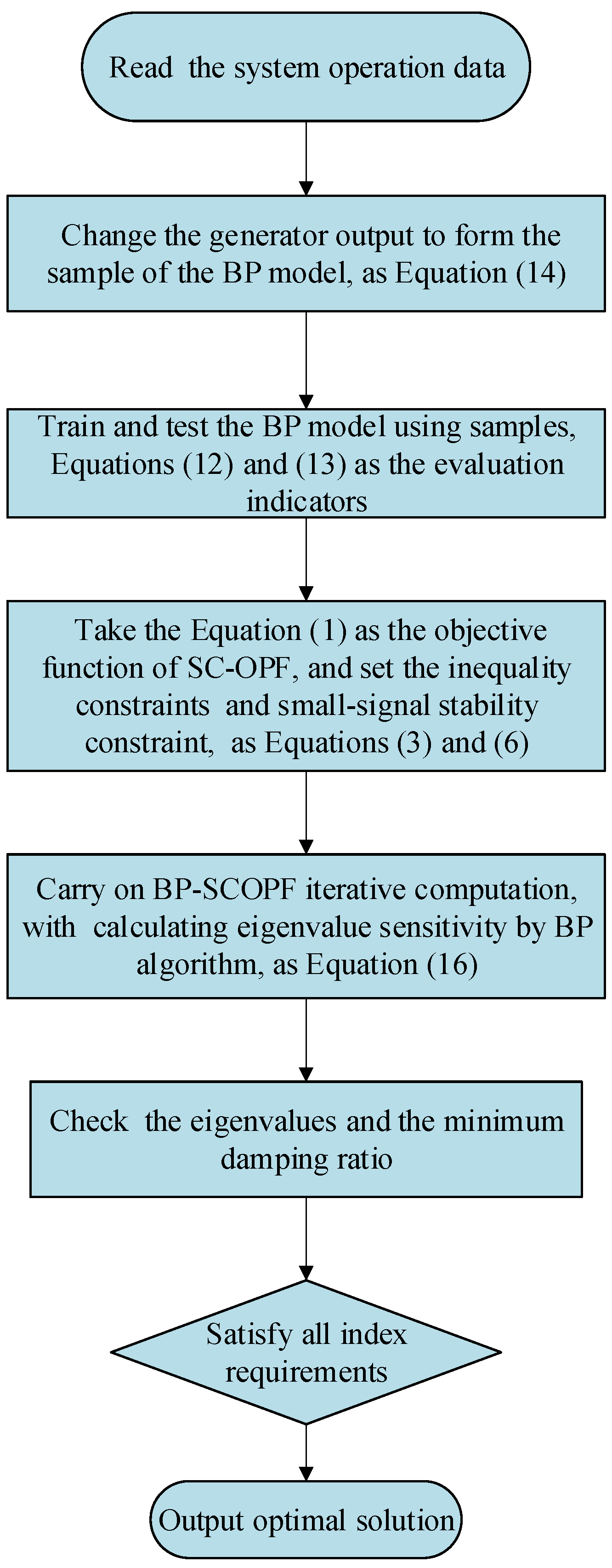
This article uses the BP neural network to optimize calculation of eigenvalue sensitivity in the SC-OPF. The specific realization steps are as follows:
  • Read the system operation data from text files;
  • Change the generator output under the principle of system power balance to obtain the input and output of the BP model, as Equation (14);
  • Train and test the BP model using samples, judging the fitting performance according to the curve, further, Equations (12) and (13) are error analysis evaluation indicators;
  • Take the Equation (1) as the objective function of SC-OPF and set the inequality constraints and small-signal stability constraint, as Equations (3) and (6);
  • Carry on the BP-SCOPF iterative computation, with calculating eigenvalue sensitivity by BP algorithm, as show in Equation (16). Predict direction and magnitude of operating parameters by the approximate sensitivity, and then optimize variables during the iterative process;
  • Check the eigenvalues and the minimum damping ratio. If all prespecified constraints are satisfied, stop the run and output the optimal solution; otherwise, return to step 3.
The model framework is shown in Figure 2.

4. Case Study

In this section, the 9-bus system is used to test the proposed model, and the 39-bus system is utilized to verify it. In both bus systems, all generators apply sixth-order models and base capacity of 100 MVA, taking into account the excitation system. The loads are modeled with constant impedance without considering the variation of system parameters. The minimum damping ratio reliability is set to ζ T = 0.03 .

4.1. The BP-SCOPF Model of WSCC-9 Bus System

Figure 3 shows the WSCC-9 bus system. The system data, voltage constraints and power constraints can be found in [9]. There are 3000 sets of samples collected, of which the ratio of training set to test set is 9:1. The generator power varies randomly and the load power fluctuates between 70% and 130%, considering the conditions of the system power balance and power limitation.
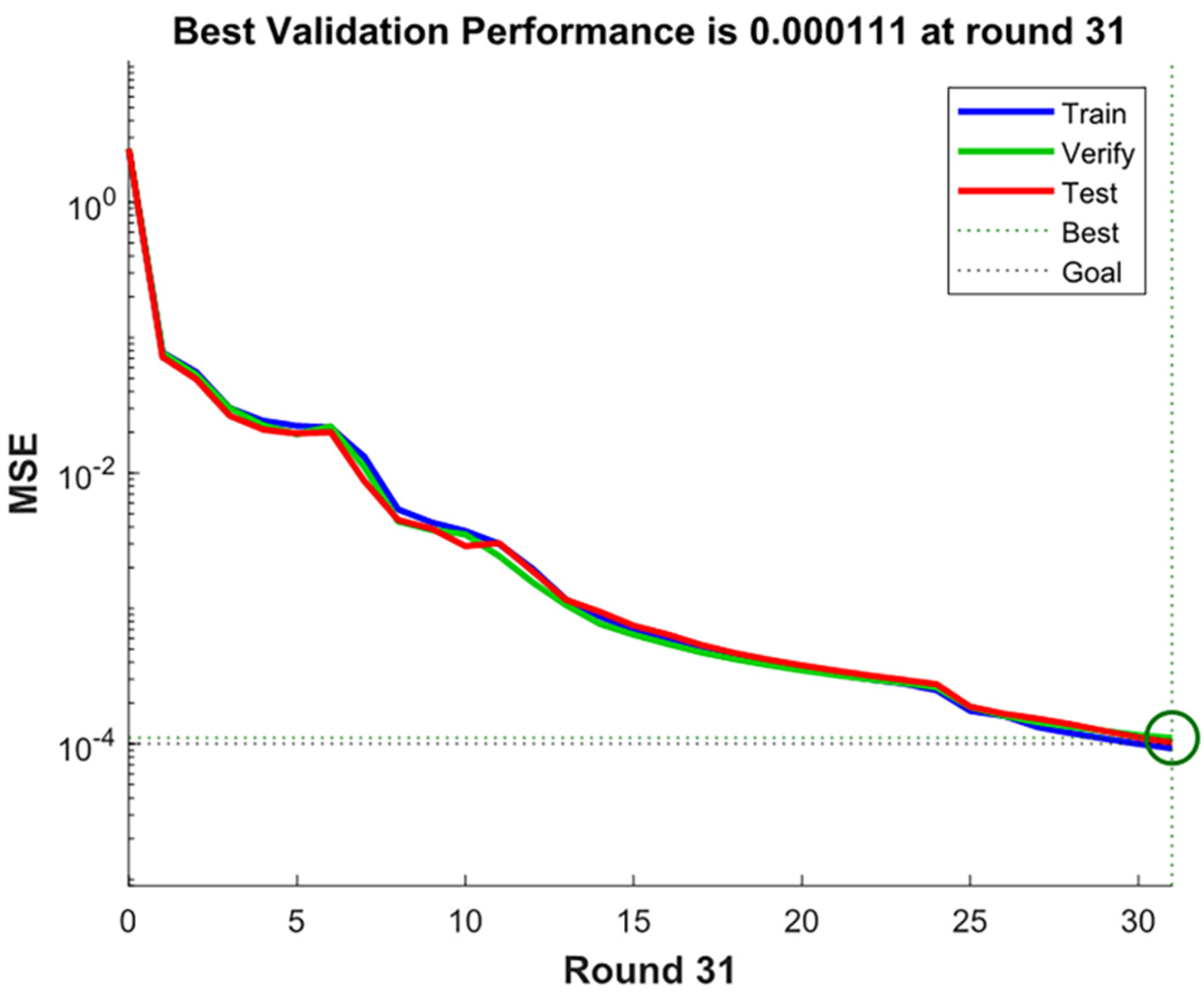
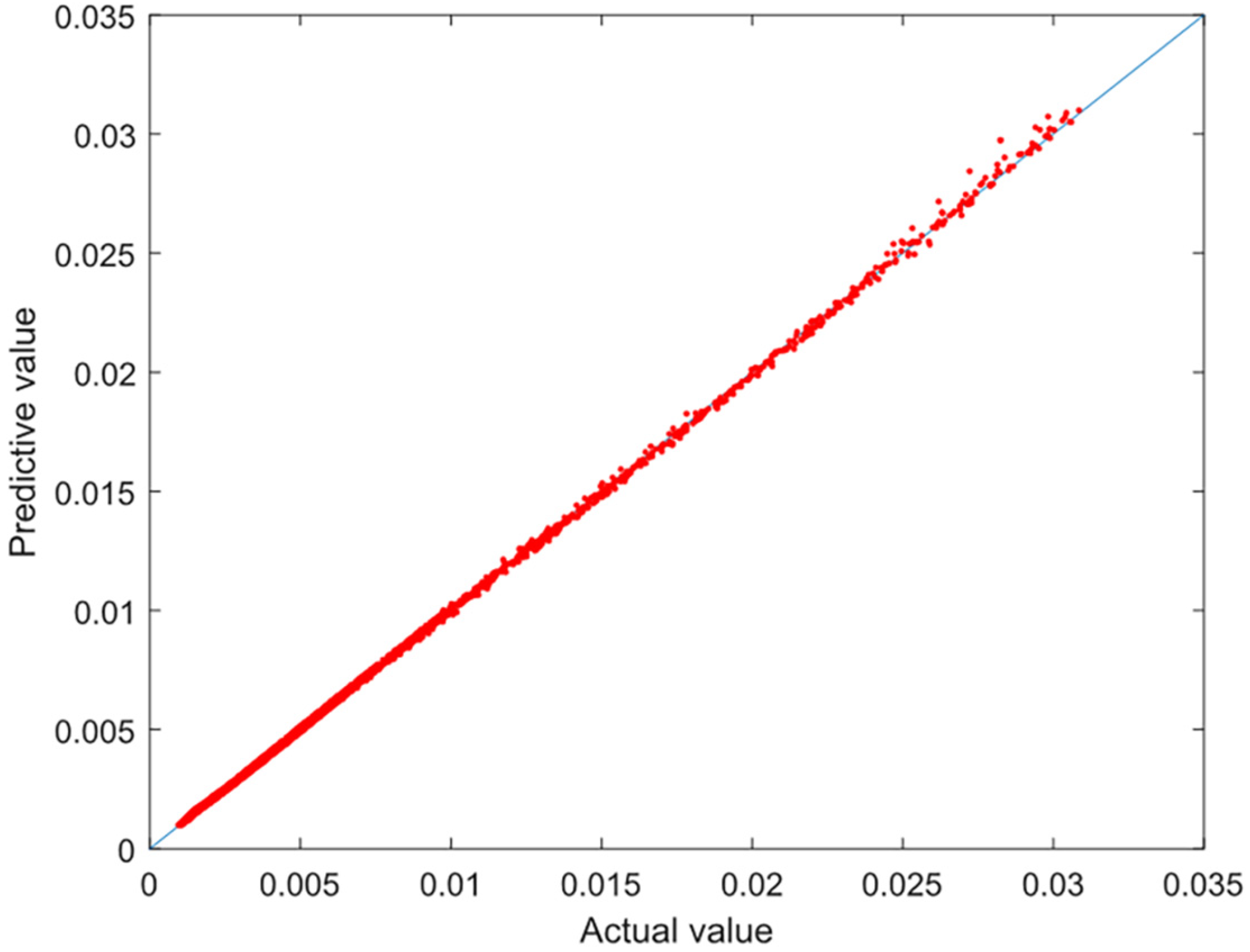
The main parameter of BP is shown in Table 1. Moreover, the network training curve is shown in Figure 4. The best validation performance is round 31. According to the error analysis, the RMSE is 4.52 × 10⁻⁵ and the MAPE is 1.56%. As seen in Figure 5, the predicted values are close to the actual values, verifying that the BP neural network has excellent mapping ability.
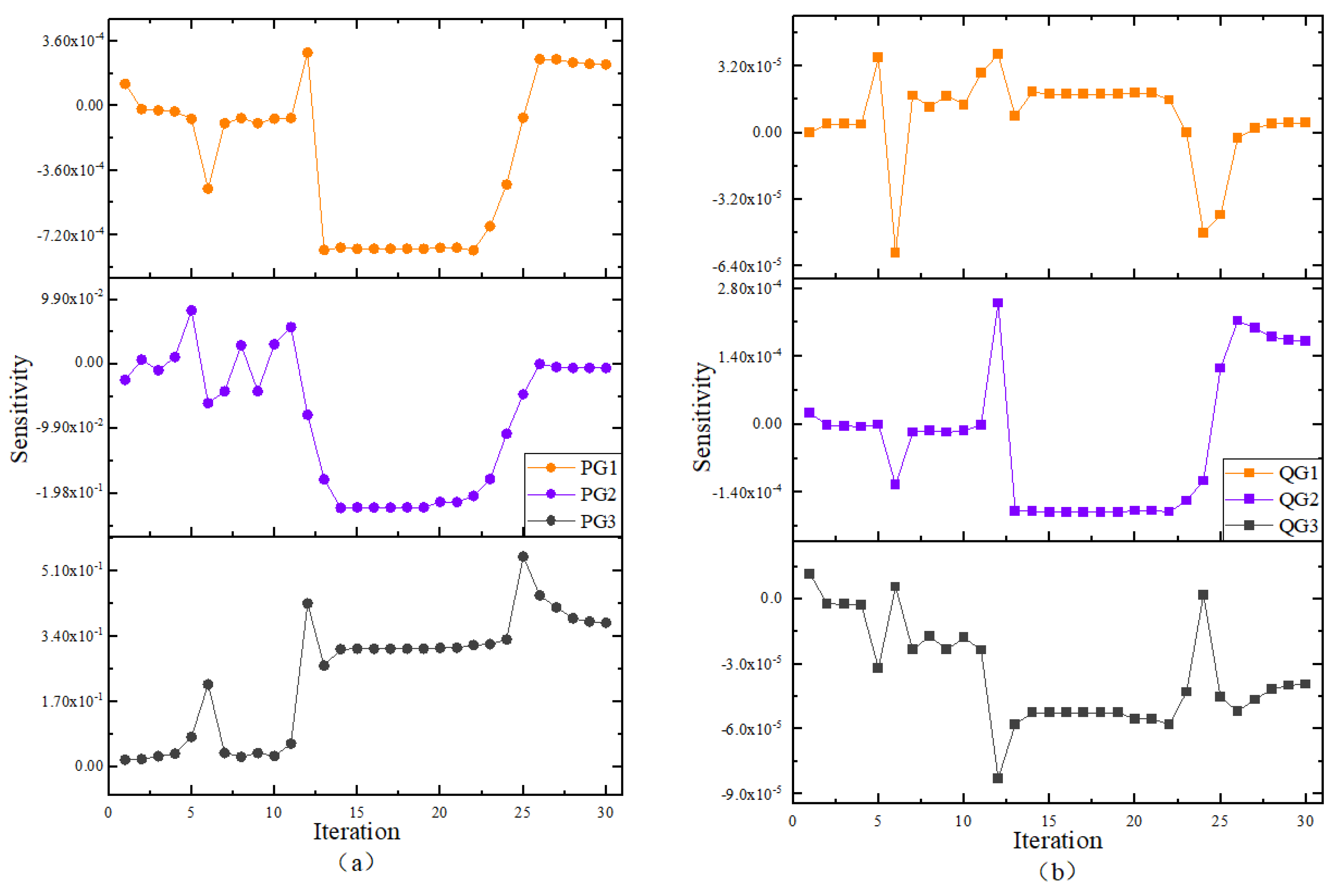
Table 2 shows the comparison results in the standard load. PF is the power flow calculation that only considers the power balance. The minimum damping ratio of PF is 0.0057, which fails to satisfy the safety requirement of 0.03. OPF is the conventional optimal power flow, and the total active power decreases 2 MW, but the minimum damping ratio is also reduced to 0.0034, which is detrimental to long-term stable operation. In the solution of BP-SCOPF, the total active power is between the results of the above methods and the critical minimum damping ratio is improved to 0.0302. The approximate sensitivity to generator over 30 iterations is shown in Figure 6. The sensitivity fluctuates widely and there is no definite pattern. The direction and magnitude of the generator changes are determined by the value of sensitivity. The sensitivity to PG2 is counted as negative 21 times, so the PG2 drops to the lower bound in the result. The sensitivity to PG3 is all larger than 0 and the sensitivity to PG1 fluctuates above and below 0, thus PG3 increases more notably than PG1. The optimal solution verifies the feasibility of BP-SCOPF method.
To further demonstrate the good performance of BP-SCOPF model, we compare five cases of different loads in the WSCC-9 bus system. Table 3 specifies the different loads, and Table 4 shows the comparison of the BP-SCOPF and conventional methods. From the results, the critical damping ratio of the BP-SCOPF model all exceeds 0.03, with a total power increase of less than 2 MW over the OPF. This explains that BP-SCOPF can ensure the small-signal stability of the system after load changes, and has good economics without the need for a large increase in generator output.

4.2. A Linear Programming Correction Model Compared with BP-SCOPF Model

To prove the superiority of the BP-SCOPF model, we envisage using a linear programming correction model common in economic scheduling to adjust the damping ratio based on the OPF results. The new model is briefly written as LPC model and is described as below:
m i n P G i P G i = P L i + P L o s s C i P G i = ζ ζ m i n + ζ ζ T P G i m i n P G i + P G i P G i m a x
where P G i is the active power change, P L o s s is the total active output loss, C i is the corresponding sensitivity of the minimum damping ratio, ζ is the adjustment amount of the minimum damping ratio.
The system parameters of the following five cases are the same as the Section 4.1. Table 5 and Table 6 show the optimal solution of LPC and BP-SCOPF model. In the Case0, the minimum damping ratio is adjusted to 0.0302 in the LPC model, but the actual value is 0.0104 after calibration. This is because the sensitivity is highly nonlinear and varies distinctly with the control variables. It is difficult to obtain the actual optimum solution using constant sensitivity of a state. In the Case2, both of the two models can contain the small-signal stability constraint, despite this, the total power of BP-SCOPF is 2.02 MW less than that of LPC, so BP-SCOPF has outstanding advantages. Case3 illustrates that the LPC model may adjust the minimum damping ratio to less than 0 causing the system to lose the small-signal stability. The analysis from Case4 shows that the minimum damping ratio rises to 0.0519 in LPC model, but the total power of LPC is 4.7 MW larger than that of BP-SCOPF, sacrificing massive economies. Compared with the LPC model, the BP-SCOPF model can go beyond the local extreme value, find the global optimum and calculate the exact optimal solution.

4.3. The BP-SCOPF Model of IEEE-39 Bus System

The BP-SCOPF method is confirmed in the 39-bus system. The upper and lower limits of bus voltages are 1.1 Pu. and 0.9 Pu., respectively. The generator set operating boundary is shown in Table 7. A total of 3000 sets of samples are collected in the model, and the power fluctuation of generators and loads is set in the same way as the WSCC-9 bus system. Table 8 shows the results of three power flow calculations. The minimum damping ratios of PF and OPF, respectively, are 0.0214 and 0.0209, neither of which could reach 0.03. After using the BP-SCOPF method, the critical damping ratio is improved to 0.0301 which ensures the power system stability and safety.
To further validate the effectiveness and accuracy of the BP-SCOPF model in the IEEE-39 bus system with different load levels, the following simulations are performed, where the load factor μ is defined as:
P L i = μ P L 0 Q L i = μ Q L 0
where P L 0 and Q L 0 , respectively, represent the active and reactive output of the standard load.
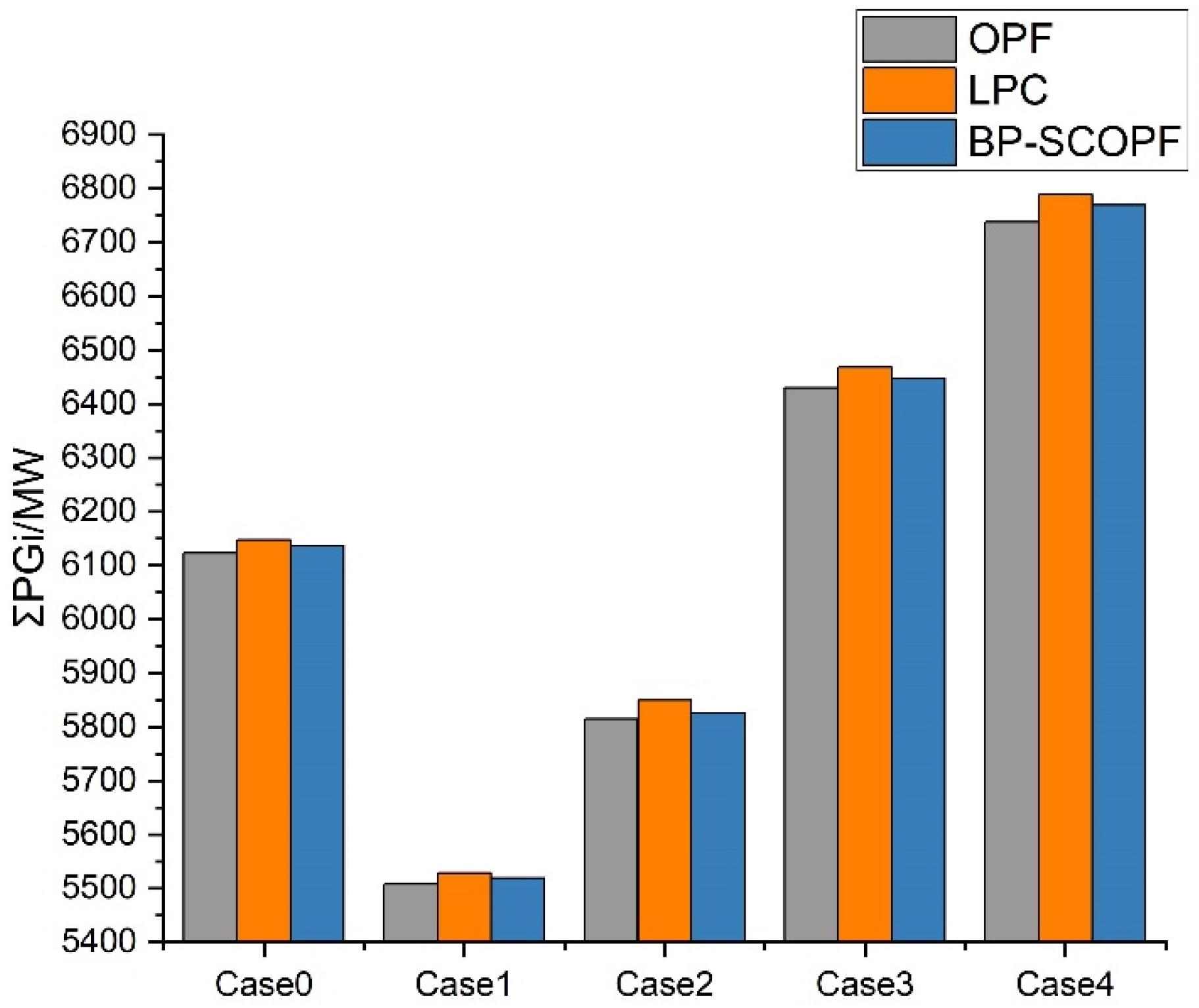
Table 9 shows the minimum damping ratios calculated in the five different load levels. Moreover, Figure 7 displays the total generator power of these five cases. The minimum damping ratios of OPF are all less than 0.03. After using the LPC model, the minimum damping ratios are increased except Case2, but only the minimum damping ratio of Case0 reaches 0.03. The minimum damping ratios of BP-SCOPF are adjusted to around 0.03 in all cases, as discussed in the 9-bus system. In all examples, the total generator power of BP-SCOPF is smaller than that of LPC and slightly larger than that of OPF, which reflects that some economy is sacrificed after considering the small-signal stability, but the total power of the BP-SCOPF method is satisfactory compared with the economically scheduled LPC method.
Table 10 provides the computational time of the 9-bus and 39-bus systems in the standard load conditions. For a deterministic system, only one training of the BP is required, as the load and generator variations are already considered in the samples, as described in Section 4.1, which reduces the memory launching the BP algorithm. The total BP-SCOPF time of 39-bus system is 19.14 s, compared with 157.38 s for the conventional method in the literature [30], which proves that the calculation speed of the proposed method is faster.

5. Conclusions

This article proposes the BP-SCOPF model considering the economics and stability of the power system. The BP neural network is firstly applied to the SC-OPF optimization step, which fills the algorithm of solving eigenvalue sensitivity problem in the OPF field. Given the complex sensitivity expression formula in the traditional interior point method, the BP neural network is introduced to optimize the calculation of sensitivity, and it makes the small-signal stability index and sensitivity more concise and flexible. The experimental results on the 9-bus and 39-bus systems show that the BP-SCOPF model can improve the critical minimum damping ratio to 0.03 and calculate the optimal solution to meet the small-signal stability. The BP algorithm accurately fits the mapping relationship between the generator power and the minimum damping ratio of the system and rapidly calculates the approximate sensitivity of the critical damping ratio in the correction equation during the BP-SCOPF iteration, which shows that the BP algorithm has the features of good nonlinear fitting, fast-fitting speed and high precision. Compared with LPC method, the BP-SCOPF method has a superior capability to break out of the partial extreme value and conduct a global search. Our future study will aim to larger power systems, consider renewable energy sources on the BP-SCOPF model, and strive to optimize BP-SCOPF to give full play to its maximum value.

Author Contributions

Conceptualization, Y.Y. and Y.L.; methodology, Y.L.; software, Y.L.; validation, Y.Y., Y.L. and L.Y.; formal analysis, Y.L.; investigation, Y.L.; resources, Y.Y.; data curation, Y.Y.; writing—original draft preparation, Y.L.; writing—review and editing, Y.L.; visualization, Y.L.; supervision, Y.Y.; project administration, L.Y.; funding acquisition, Y.Y. All authors have read and agreed to the published version of the manuscript.

Funding

This work was supported in part by Guangxi Special Fund for Innovation-Driven Development under Grant AA19254034 and in part by Guangxi Key Laboratory of Power System Optimization and Energy Technology Research Grant.

Institutional Review Board Statement

Not applicable.

Informed Consent Statement

Not applicable.

Data Availability Statement

Not applicable.

Conflicts of Interest

The authors declare no conflict of interest.

References

  1. Liao, S.; Xu, J.; Sun, Y.; Bao, Y.; Tang, B. Control of energy-intensive load for power smoothing in wind power plants. IEEE Trans. Power Syst. 2018, 33, 6142–6154. [Google Scholar] [CrossRef]
  2. Ali, M.A.; Kamel, S.; Hassan, M.H.; Ahmed, E.M.; Alanazi, M. Optimal Power Flow Solution of Power Systems with Renewable Energy Sources Using White Sharks Algorithm. Sustainability 2022, 14, 6049. [Google Scholar] [CrossRef]
  3. Shafiullah, M.; Rana, M.J.; Shahriar, M.S.; Zahir, M.H. Low-frequency oscillation damping in the electric network through the optimal design of UPFC coordinated PSS employing MGGP. Measurement 2019, 138, 118–131. [Google Scholar] [CrossRef]
  4. Yang, D.; Wang, W. On-line active power modulation based on multi-variable damping ratio sensitivity. Power Syst. Technol. 2017, 41, 3612–3619. [Google Scholar] [CrossRef]
  5. Li, H.; Liu, S.; Ji, H.; Yang, D.; Yang, C.; Chen, H.; Chen, Z. Damping control strategies of inter-area low-frequency oscillation for DFIG-based wind farms integrated into a power system. Int. J. Electr. Power Energy Syst. 2014, 61, 279–287. [Google Scholar] [CrossRef]
  6. Chabane, Y.; Ladjici, A.A.; Hellal, A.; Dookhitram, K. Cooperative coevolutionary algorithms for optimal PSS tuning based on Monte-Carlo probabilistic small-signal stability assessment. Int. Trans. Electr. Energy Syst. 2020, 30, e12618. [Google Scholar] [CrossRef]
  7. Zecevic, A.; Miljkovic, D. The effects of generation redispatch on hopf bifurcations in electric power systems. IEEE Trans. Circuits Syst. I Fundam. Theory Appl. 2002, 49, 1180–1186. [Google Scholar] [CrossRef]
  8. Li, S.; Chiang, H. Continuation power flow with multiple load variation and generation re-dispatch patterns. In Proceedings of the 2006 IEEE Power Engineering Society General Meeting, Montreal, QC, Canada, 18–22 June 2006. [Google Scholar]
  9. Condren, J.; Gedra, T. Expected-security-cost optimal power flow with small-signal stability constraints. IEEE Trans. Power Syst. 2006, 21, 1736–1743. [Google Scholar] [CrossRef]
  10. Saric, A.; Stankovic, A. Rapid small-signal stability assessment and enhancement following changes in topology. IEEE Trans. Power Syst. 2015, 30, 1155–1163. [Google Scholar] [CrossRef]
  11. Li, P.; Wei, H.; Bai, X. Small-signal stability constrained optimal power flow based on NLSDP. Proc. Csee. 2013, 33, 69–76. [Google Scholar] [CrossRef]
  12. Li, P.; Qi, J.; Wang, J.; Wei, H.; Bai, X.; Qiu, F. An SQP method combined with gradient sampling for small-signal stability constrained OPF. IEEE Trans. Power Syst. 2016, 32, 2372–2381. [Google Scholar] [CrossRef] [Green Version]
  13. Li, Y.; Geng, G.; Jiang, Q.; Li, W.; Shi, X. A sequential approach for small signal stability enhancement with optimizing generation cost. IEEE Trans. Power Syst. 2019, 34, 4828–4836. [Google Scholar] [CrossRef]
  14. Deepak, P.; Ramtin, M.; Tuncay, A.; Ali, D. Small-Signal Stability-Constrained Optimal Power Flow for Inverter Dominant Autonomous Microgrids. IEEE Trans. Ind. Electron. 2021, 69, 7318–7328. [Google Scholar] [CrossRef]
  15. Duong, T.L.; Nguyen, N.A.; Nguyen, T.T. A Newly Hybrid Method Based on Cuckoo Search and Sunflower Optimization for Optimal Power Flow Problem. Sustainability 2020, 12, 5283. [Google Scholar] [CrossRef]
  16. Zhou, Y.; Zhang, B.; Xu, C.; Lan, T.; Diao, R.; Shi, D.; Lee, W.J. A data-driven method for fast ac optimal power flow solutions via deep reinforcement learning. J. Mod. Power Syst. Clean Energy 2020, 8, 1128–1139. [Google Scholar] [CrossRef]
  17. Jia, Y.; Bai, X. A CNN approach for optimal power flow problem for distribution network. In Proceedings of the 2021 Power System and Green Energy Conference (PSGEC), Shanghai, China, 20–22 August 2021; pp. 35–39. [Google Scholar]
  18. Pan, X. Deepopf: Deep neural network for dc optimal power flow. In Proceedings of the 8th ACM International Conference on Systems for Energy-Efficient Buildings, Cities, and Transportation, Wuhan, China, 17 November 2021; pp. 250–251. [Google Scholar]
  19. Li, S.; Goel, L.; Wang, P. An ensemble approach for short-term load forecasting by extreme learning machine. Appl. Energy 2016, 170, 22–29. [Google Scholar] [CrossRef]
  20. Zhao, J.; Nguyen, H.; Nguyen-Thoi, T.; Asteris, P.; Zhou, J. Improved levenberg–marquardt backpropagation neural network by particle swarm and whale optimization algorithms to predict the deflection of rc beams. Eng. Comput. 2021, 1–23. [Google Scholar] [CrossRef]
  21. Rumelhart, D.; Hinton, G.; Williams, R. Learning representations by back-propagating errors. Nature 1986, 323, 533–536. [Google Scholar] [CrossRef]
  22. Vankayala, V.; Rao, N. Artificial neural networks and their applications to power systems—A bibliographical survey. Electr. Power Syst. Res. 1993, 28, 67–79. [Google Scholar] [CrossRef]
  23. Huang, S.; Wu, Q.; Liao, W.; Wu, G.; Li, X.; Wei, J. Adaptive Droop-Based Hierarchical Optimal Voltage Control Scheme for VSC-HVDC Connected Offshore Wind Farm. IEEE Trans. Ind. Inf. 2021, 17, 8165–8176. [Google Scholar] [CrossRef]
  24. Huang, S.; Zhang, J.; He, Y.; Fu, X.; Fan, L.; Yao, G.; Wen, Y. Short-Term Load Forecasting Based on the CEEMDAN-Sample Entropy-BPNN-Transformer. Energies 2022, 15, 3659. [Google Scholar] [CrossRef]
  25. Feilat, E. Neural network based assessment of small-signal stability. Int. J. Model. Simul. 2007, 27, 151–157. [Google Scholar] [CrossRef]
  26. Yang, Y.; Zhang, X.; Yang, L. Data-driven power system small-signal stability assessment and correction control model based on XGBoost. Energy Rep. 2022, 8, 710–717. [Google Scholar] [CrossRef]
  27. Xiao, Z.; Ye, S.; Zhong, B.; Sun, C. BP neural network with rough set for short term load forecasting. Expert Syst. Appl. 2009, 36, 273–279. [Google Scholar] [CrossRef]
  28. Xu, X.; Peng, L.; Ji, Z.; Zheng, S.; Tian, Z.; Geng, S. Research on Substation Project Cost Prediction Based on Sparrow Search Algorithm Optimized BP Neural Network. Sustainability 2021, 13, 13746. [Google Scholar] [CrossRef]
  29. Chung, C.Y.; Wang, L.; Howell, F.; Kundur, P. Generation rescheduling methods to improve power transfer capability constrained by small-signal stability. IEEE Trans. Power Syst. 2004, 19, 524–530. [Google Scholar] [CrossRef]
  30. Zarate, R.; Milano, F.; Conejo, A. An OPF methodology to ensure small-signal stability. IEEE Trans. Power Syst. 2010, 26, 1050–1061. [Google Scholar] [CrossRef]
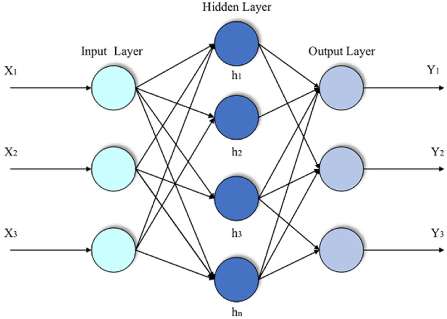
Figure 1. The architecture of the BP algorithm.
Sustainability 14 13386 g001
Figure 2. The flow chart of BP-SCOPF Model.
Sustainability 14 13386 g002
Figure 3. Topology diagram of the WSCC-9 bus power system.
Sustainability 14 13386 g003
Figure 4. BP network training performance.
Sustainability 14 13386 g004
Figure 5. Actual values and predicted values of BP.
Sustainability 14 13386 g005
Figure 6. (a) Sensitivity of the minimum damping ratio to generator active power. (b) Sensitivity of the minimum damping ratio to generator reactive power.
Sustainability 14 13386 g006
Figure 7. The total generator power of five cases.
Sustainability 14 13386 g007
Table 1. The main parameter of BP neural network in BP-SCOPF.
ParameterSet Value
Maximum iterations100
Learning rate0.01
Goal accuracy0.001
Input layer neurons 30
Hidden layer neurons9
Output layer neurons1
Table 2. Comparison results of three power flow calculation in the standard load.
ζΣPGi
/MW
PG1
/MW
PG2
/MW
PG3
/MW
QG1
/Mvar
QG2
/Mvar
QG3
/Mvar
PF0.0057319.6471.641638527.106.59−10.92
OPF0.0034317.64156.2388.5772.8415.203.82−10.42
BP-SCOPF0.0302319.19123.2025170.9927.452.62−2.39
Table 3. Five cases of different loads in the WSCC-9 bus system.
PL1/MWPL2/MWPL3/MW
Case012590100
Case1110110110
Case2130100120
Case3150110130
Case4160115125
Table 4. Comparison of three power flow calculation with different loads.
PFOPFBP-SCOPF
ζPFΣPGi/MWζOPFΣPGi/MWζBPΣPGi/MW
Case00.0057319.640.0034317.640.0302319.19
Case10.0065334.490.0054332.920.0306334.23
Case20.0071354. 410.0056353.170.0303354. 31
Case30.0083395.660.0067393.980.0305394.98
Case40.0105406.060.0074404.310.0308405.29
Table 5. The optimal solution of LPC model.
ζLPCζCheckΣPG/MWPG1/MWPG2/MWPG3/MW
Case00.03020.0104320.3412590100
Case10.03050.0218335.94110110110
Case20.03010.0306356.43130100120
Case30.0306−1398.09150110130
Case40.03110.0519410.76160115125
Table 6. The optimal solution of BP-SCOPF model under the same system conditions.
ζBP-SCOPFζCheckΣPGi
/MW
PG1
/MW
PG2
/MW
PG3
/MW
QG1
/Mvar
QG2
/Mvar
QG3
/Mvar
Case00.03010.0302319.19123.2025170.9927.452.62−2.39
Case10.03010.0306334.23129.7732.67171.7927.492.15−1.30
Case20.02990.0303354.41136.6747.03170.7129.693.44−0.91
Case30.03070.0305394.98173.0552.75169.1836.856.11.34
Case40.03040.0308405.29183.2253.86168.2140.156.631.6
Table 7. The generator set operating boundary.
Gen1Gen2Gen3Gen4Gen5Gen6Gen7Gen8Gen9Gen10
P Gi min /MW175355.6455355.6442.4355.6392378581700
P Gi max /MW402.5747.5920862.5862.5862.5862.580510351380
Q Gi min /Mvar−249.4−463.2−570.1−534.5−463.2−534.5−534.5−498.8−641.4−855.2
Q Gi max /Mvar249.4463.2570.1534.5463.2534.5534.5498.8641.4855.2
Table 8. Comparison results of different power flow calculation.
PFOPFBP-SCOPF
PGi/MWQGi/MvarPGi/MWQGi/MvarPGi/MWQGi/Mvar
Gen1250203.97402.5−42.29402.5181.84
Gen2522.28238.40747.5398.90355.60208.73
Gen3650251.59614.42193.14455218.51
Gen4632152.53442.4572.78767.56181.04
Gen5508185.53462.15120.30499.17194.50
Gen6650266.36770.57191.15455281.60
Gen7560131.7039232.10862.5250.2
Gen854045.01421.505.88378−57.26
Gen9830140.99582.03−53.5958199.73
Gen101000239.821287.208.391380216.01
ΣPGi/MW6142.286122.326136.33
ζ0.02140.02090.0301
Table 9. The minimum damping ratios with five load levels.
Case0Case1Case2Case3Case4
μ 10. 90.951.051.10
ζOPF0.02090.01860.01940.02200.0235
ζLPC after check0.03080.02460.01760.02850.0261
ζBP-SCOPF after check0.03010.02940.03050.02960.0302
Table 10. The computational time of the procedure iterations.
BP Training/s Iteration Round Average
Iteration/s
Total
BP-SCOPF/s
9-bus system1.36300.175.12
39-bus system2.01580. 3319.14
Publisher’s Note: MDPI stays neutral with regard to jurisdictional claims in published maps and institutional affiliations.