Abstract
The present work describes a multi-area (two and three) renewable-energy-source-integrated thermal-hydro-wind power generation structure along with fleets of plug-in electrical vehicles (PEVs) in each control area. The generation–load balance is the prime objective, so automatic generation control (AGC) is adopted in the system. In the paper, a cascaded combination of proportional derivative with filter PDN and fractional-order proportional integral (FOPI) is proposed and tuned using the hybrid chemical reaction optimization with pattern search (hCRO-PS) algorithm. The hCRO-PS algorithm is designed successfully, and its effectiveness is checked through its application to various benchmark functions. Further, Eigen value analysis is carried out for the test system to verify the system stability. The impacts of diverse step load perturbation (i.e., case I, II, III, and IV) and time-varying load perturbation are also included in the study. Moreover, the impact of renewable sources, PEVs in different areas, and varied state of charge (SOC) levels on the system dynamics are reflected in the work. From the analysis, it can be inferred that the proposed controller provides comparable results with other fractional-order and conventional controllers under varying loading conditions.
1. Introduction
The electrical power sector is highly complex in nature due to the presence of generators, transmission lines, distribution systems, protective equipment, and a large variety of connecting loads with its associated interconnections. Even in small-scale frequency variation due to changing loads, the power system is always prone to producing huge undesirable variation in the output, and the quality of power is also distorted. So, the deviation of frequency must be abated for the optimum and efficient operation of a power system. Generally, any disproportion in the generation–demand balance initiates frequency variation, which is absolutely unacceptable [1]. Thus, automatic generation control becomes essential for the power system to maintain the system within the stability constraints of generation–demand. It also regulates the active and reactive power which is produced from varied controllable sources. The disturbances in one area of the network are sometimes spared to healthier areas, rapidly causing the instability of the system and sometimes leading to the cascading outage/blackout of part or all of the system [2]. Hence, it is recommended to incorporate AGC in the system. The stability is crosschecked by observing and limiting the frequency and tie line exchange power within minimal predefined specifications [3]. AGC can certainly make sure that a system does not work under the impact of prolonged frequency variation after a load disturbance takes place and the response reaches a to stable state at the earliest time.
To analyze the effect of AGC on isolated systems as well as inter-related systems, various research articles are available. Elgerd et al. [4] first proposed the concept of AGC in the thermal model. Later, Nanda et al. [5] extended this study to a two-area hydro thermal system with the generation rate constraint (GRC) as non-linearity in the system. The same author also performed the analysis of AGC in a three-unequal-area system, incorporating GRC and a non-reheat turbine of a thermal plant [6]. Adding another non-linearity called Governor Dead Band (GDB), Gozde et al. [7] studied it in a two-area hydro model. However, Sahu et al. [8] used several non-linearity aspects such as boiler dynamics (BD), GDB, and GRC to draw a conclusion from a two-area, complex and realistic power system model. Bhatt et al. [9] attempted to analyze the system response with diversified sources such as hydro-thermal-diesel. Saikia et al. [10] further studied it in an interconnected single reheat system and then applied it to a five-area system. However, due to the drawbacks of carbon discharges, it urgently needed to be replaced by integrating renewable energy sources to the existing system to generate adequate demand power. Sopian et al. [11] discussed a hybrid wind–solar model with its design and possibility for household application. For the grid integration of solar power, Kadri et al. [12] discussed the variety of possibilities and methodologies with maximum power point tracking. A case study of the islands of Samso and Orkney was considered to establish the enhancements achieved through the application of Demand-Side Management actions to the available renewable energy sources and curtailment events [13]. On the other hand, plug-in electric vehicles (PEVs) represent one of the distributed energy sources, gaining popularity as they do not rely on fossil fuel, thus contributing to a clean environment by reducing the greenhouse gas emissions. Debaramma et al. [14] used PEVs in a deregulated environment and analyzed their response with fractional-order controller configuration. Padhy et al. [15] attempted to assess the performance of PEVs in a two-area model with a cascade controller. Saha et al. [16] further extended the study by including renewable sources and time delay. A method for day-ahead optimal dispatch estimation considering wind turbines, photovoltaic panels, battery energy storage systems, and electric vehicles (EVs) in a smart grid scenario was studied [17]. The application of V2G (Vehicle to Grid) technology improves the grid-side peak-to-valley ratio, significantly and simultaneously benefiting the users and the power system [18].
The amplified complications of power structures necessitate an effective controller in governor systems of AGC to efficiently achieve objectives. Different generalized controllers such as integral (I), proportional integral (PI), and proportional integral derivative with filter (PIDN) suggested in the discussed literature were considered in previous works. Elgerd et al. [4] used a basic I controller in their study, while Nanda et al. [5] used I and PI as a secondary controller. Apart from this type of controller, higher-degree-of-freedom (DOF) integer-order (IO) controllers, fractional-order (FO) controllers, and cascade controllers are gaining popularity in AGC studies for the smooth maintenance of frequency [15,16]. Morsali et al. [19] reported the use of an FOPID controller in a two-area AGC model with the presence of a saturation limit. The presence of the same controller can be found in [20], where the author used a non-reheat thermal model in an AGC system. Recently, Saha et al. [16] used a combination of two different controllers (PIDN- FOPD) in a deregulated AGC network. However, a cascading proportional derivative with filter (PDN) with a fractional-order PI controller can be used in a system in a secondary control loop, whose characteristics performance is studied in neither classical AGC models nor in deregulated environments. Thus, we were motivated to investigate this cascaded controller in the proposed test model.
The recent literature reveals that most of papers considered a single controller as opposed to a secondary controller. However, much fewer papers explored the effectiveness of cascaded controllers in the field of AGC under conventional generators. Moreover, most studies show the effect of GRC and GDB, while only few of the studies related to AGC seem to have boiler dynamics as a non-liberality and the effect of PEVs. Thus, in the present work, a combination of a cascaded controller (i.e., PDN-FOPI) is considered with the presence of non-linearity ( i.e., GDB, GRC, and BD) along with a renewable unit (wind turbine generator) and PEVs.
The effectiveness of a controller is decided using its optimal values of gains and tuning parameters. The optimal value of the controller is gained by applying diverse meta-heuristic optimization techniques. In the past literature, a genetic algorithm was used by Bhatt et al. [9], a bacteria foraging algorithm by Saikia et al. [10], a hybrid optimization algorithm by Kumar et al. [21], flower pollination techniques by Debarama et al. [14], Modified Grey Wolf Optimization by Padhy et al. [15], a whale optimization algorithm by Saha et al. [16], and improved particle swam optimization by Chang et al. [22] to tune the controller parameter for optimum gain. Thus, it seems from the research articles that the design of a controller along with the tuning technique preferred for the generation of an array of optimal controller constraints essentially affects the operation of the system.
Motivation
It is observed from the literature survey of AGC that most of the work tuned the respective controller gains and other parameters under nominal conditions i.e., a disturbance (step load perturbation (SLP)) of 1% in the control area. However, some other uncharacteristic conditions may have an effect on system dynamics and hence the controller parameters. To check the robustness/sensitivity of the proposed controller, a large SLP (up to 10%) and other conditions such as dynamic loading, the effect of PEVs on the system response, and the outcome of state of charge (SOC) at 0.75, 0.85, and 1 was considered in the test system. Moreover, Eigen value analysis was included in the proposed study with regard to the system stability, which was not reported in previous studies.
Traditional and classical optimization algorithms have disadvantages, e.g., the solution is confined in local optima, in addition to a slow convergence rate. This problem is overridden by using a modified cascade optimization algorithm. The proposed hybrid CRO-PS performs the exploration and exploitation of the optimal solution separately using two different sets of equations. Thus, it shows reduced chances of getting trapped in local optima and has high convergence when applied to a multi-source system. The high complexity and contradictory performance parameters in the system make it difficult for the optimization technique to converge and reach an optimal solution. Thus, the application of the hCRO-PS technique to a multi-source system needs to be verified. The contributions of the present work can be presented as follows:
- 1.
- A multi-source test system is designed considering non-linearity and PEV, with extension to a three-area system.
- 2.
- An efficient optimization technique is developed for application to the designed system, and it is verifed through unconstrained and constrained benchmark functions.
- 3.
- An efficient controller structure is designed for the regulation of the two-area/three-area system.
- 4.
- Stability analysis of the system with PEVs, different SOCs, and time varying loads is performed.
- 5.
- Efficient minimization of variation in frequency post system perturbations.
In Section 2, the two-area power system with renewable units and PEVs is considered by mathematically formulating the transfer function for each unit. Here, various constraints and their limits are also discussed. The steps in the formulation of the objective function (J) are discussed in Section 3. An improved optimization technique named the hCRO-PS algorithm is shown in Section 4, and its effectiveness is verified against various constrained and non-constrained benchmark functions. The design approach of a modified cascaded controller through mathematical derivation is presented in Section 5. The system stability and performance evaluation of a two-area system is presented in Section 6 with the help of mathematical indices and figures. Then, the study is further extended to a three-area system reflected in Section 7. The performance and stability analysis of the three-area system is presented in Section 8 by considering varied testing conditions, and the results are equated to similar work conducted by other researchers. The concluding remarks of the work are briefly discussed in Section 9. Finally, all the parameters considered in the test systems depicted in Section 2 and Section 8 are presented in Appendix A.
2. System Investigation
The model considered in the analysis covers conventional power plants such as thermal- and hydro- as well as renewable-based power plants (wind turbine generator), along with fleets of PEVs, as shown in Figure 1. The thermal and hydo power plant are considered base load power plants and produce 70 to 80% of total energy demand in developing countries such as India [23]. The thermal and hydro plant considered in the study is non-linear in nature as it contains several non-linearities such as Governor Dead Band (GDB), boiler dynamics (BD) and generation rate constraint (GRC) [24]. GDB is defined as the minimum time required for the start of the operation of mechanical devices. As in the rack and pinion arrangement, mechanical devices are involved, which organize the rotatory motion to open/close the valve, which causes GDB. Thus, it affects the operation of the control valves, and unusual variations in speed may occur even before any change in valve position. In the thermal and hydro plant, 0.05% and 0.02% of GDB is used, respectively. To sense the pressure and flow of steam in any unintentional circumstances, boiler dynamics (BD) is integrated in a thermal system so that supervisory action is commenced in the turbine and boiler control taps. The generation rate for either raising the generation or lowering the generation is usually predefined for a generating unit and known as GRC. So, a GRC of 3% per min for a thermal plant and 270% per minute for rising generation along with 360% per minute for lowering generation is reflected in the hydro model [8].
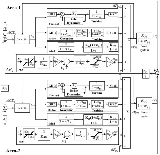
Figure 1.
Block diagram model with transfer function for multi-source 2-area system.
The power derived from a renewable based power plant such as a wind turbine generator is purely dependent upon nature, as the input is wind speed. So, the efficiency of this type of plant is low and inconsistent, because wind speed is not predictable. However, cheap energy can be harvested from this type of plant by implementing various control techniques. The productivity of a wind plant can be enhanced by integrating power set point control and a hydraulic actuator, which also improves the efficiency [25]. The overall transfer function of a wind system model with a hydraulic pitch actuator is depicted in Equation (1).
PEVs represent one distributed energy storage technology that is expected to play a vital role in grid power management and in emergency dependability facilities due to the advancement of vehicle-to-grid (V2G) technology. At same time, the popularity and dependability of EVs are increasing as the decline in the necessity for petrol and greenhouse emissions contributes to a healthy and safe atmosphere [16]. By implementing PEVs for primary frequency regulation, the following benefits can be realized in contrast with traditional AGC units:
- 1.
- The control amplitude signal response and its polarity is restricted in AGC plants, while in PEVs, this restriction can be eliminated by using advanced power electronic equipment.
- 2.
- Any major modification in thermal power plants may lead to increments in cost and reduced life spans, but in the case of PEVs, the time constant is very small, so the response stabilizes rapidly. Thus, it can decrease the requirement of thermal generators in terms of the energy capacity limit.
- 3.
- When PEVs participate in ancillary services, the variation in the charging of batteries is pretty nominal, whereas in the case of energy market management, the charging state of the battery varies significantly. Thus, the adverse effect on battery life can be reduced and the efficiency is maximized if it is connected to the grid only for the provision of ancillary services. Along with increased battery life and efficiency, economic advantages are also associated with the energy transaction. Thus, PEV owners are encouraged to register their vehicles for assistance in energy trading.
The EV model is composed of a battery charger, primary frequency control (PFC), and load frequency control (LFC). The battery charger helps the relative power flow between the grid and battery storage. To restrict the undesired frequency response during the sudden disconnection, an upper limit () and lower limit () of mHz is considered in the system. However, the value of the aggregate droop characteristics () is the same as that of conventional units (i.e., 2.4 Hz/p.u.). and refer to the EV gain and time constant, respectively, and purely depend upon the EVs’ state of charge (SOC). The value of SOC is generally varied from and is taken as 1 with respect to SOC. The incremental change in the power generation of EV fleets for area is represented by . The maximum and minimum derived power from EV fleets are referred to as and , otherwise known as upward and downward reserves, respectively. The same is calculated by the following Equations (2) and (3):
In Equations (2) and (3), the number of electric vehicles is noted as . For the proposed study, 2000 EVs are considered in each area. Figure 1 describes the complete transfer function of the EV model. For investigation purposes, the charging and discharging limit is considered as kW. However, the range can go beyond 50 kW or higher in the case of a rapid start [14].
3. Objective Function Formulation
For the better selection of an optimal controller, the selection of an appropriate objective function is a necessary and essential process. A conventional controller design is reflected in traditional cost functions such as the Integral of Time multiplied by Absolute Error (ITAE), the Integral of Absolute Error (IAE), the Integral of Time Multiplied by Square Error (ITSE), and the Integral of Square Error (ISE) [26]. However, with the advancement of complex and cascade controllers, the cost is not provided in the desired system response post disturbances. An objective function, namely Integral Square Time Multiplied by Square Error (ISTSE), having characteristics of both ITAE and ITSE, is considered. The ITAE criterion effectively controls the settling time as it is more sensitive than other criteria such as IAE and ISE, whereas ISTSE provides excellent step response [27]. Hence, ISTSE becomes an obvious choice as it produces the response with the least oscillation and overshoot.
Furthermore, to enhance the system response dynamics, a multi-objective cost function is formed by combining three individual cost functions. The deciding factor on which multi-objective function formed is the maximum deviation in frequency and time taken to settle in all the respective areas and the incremental flow of power within the area through the tie line. Moreover, the shortcomings of the single-objective function can be minimized by cascading numbers of single-objective functions to form a better-performing multi-objective function. Hence, this paper refers to the newly formed multi-objective function for tuning of the controller parameter.
The first objective function () is formulated by considering the effect of the peak overshoot of deviation in frequency in area-1 and 2 (, ), as well as deviation of the relative flow of power in the tie line (), which is depicted in Equation (4). The primary concern when choosing overshoot for is that the damping ratio regulation is portioned to the control of overshot; hence, in post disturbance, the system remains stable. Similarly, for , the settling time of the frequency deviation of area-1 and 2 (, ) along with the deviation of the relative flow of power in the tie line () is considered, as shown in Equation (5). basically keeps an additional check over the time consumed to maintain balance between generation and demand in both the area as well as the exchange power in between areas after being subjected to disturbances. In the proposal, the ISTSE cost function depicted in Equation (6) leads to better tuning by the optimization algorithm. ISTSE involves deviation in the frequency of area-1 (), area-2 () and deviation in the tie-line exchange power () to find the error function value. is the simulation time of , and in Equation (6). The third objective function is the ISTSE function, which is found to generate the controller parameter with improved system performance.
By combining the three Equations (4)–(6), a multi-objective function is formed, which has the characteristics of all the three cost functions and is mathematically depicted in Equation (7).
In which , , and are the associated gains of the respective cost function, which signifies the effectiveness of the individual functions and their contribution to the multi-objective function and must satisfy Equation (8).
Determination of Weight through Analytic Hierarchy Process (AHP)
The AHP [28] is an analytic technique that aids the user in the process of decision making through settlement using priorities. Estimating the geometric mean produces the values of associated weights. The initial step in the AHP is to produce a pairwise comparison matrix , where n is the number of parameters considered. are the elements of An n representing the relative significance of ith with respect to the jth parameter. If , the ith parameter is more significant; similarly, if , then the ith parameter is less significant as compared to other parameters. The relative normalized weights can be computed as in Equation (9).
4. Optimization Technique
4.1. Chemical Reaction Optimization (CRO)
A new type of optimization algorithm based on behavioral aspects of molecules and their interaction to reach a stable state with the lowest possible potential energy () was proposed by Albert Y.S. Lam in 2010 and called the chemical reaction optimization (CRO) [29]. The pathway that the molecules follow to reach the stable state can be utilized in the design of optimization processes. By dissipating or accepting a packet of energy, the molecules reach the stable state, which is the primary objective. The approach proclaimed that it is more effective to solve a complex problem in a stimulated time period with a large number of datasets. In CRO, molecules denote an atom group’s (variables to be optimized) energy state () (summation of potential and kinetic energy) for each molecule, characterized by its fitness value. The same can be represented by a function f with molecular structure (W), as shown below:
The potential energy surface (PES) of CRO is large, so it is difficult to find the lowest . To overcome this difficulty, it has to be directed by following two stages of operation. The first stage is intensification, where lower for each molecule are finalized in which the on-wall ineffective collision and inter-molecular collision steps are involved, and if it fails to perform, then the diversification step is executed, and a new distant search space is chosen instantly. Decomposition and synthesis help the molecules to diversify further until the lowest PE state is attained.
In the process of CRO, a molecular structure may be varied, which can effect on-wall or inter-molecular ineffective collision, decomposition, and synthesis reactions. In the variation process, the structure of molecules may vary from w to w* and is acceptable if it satisfies the condition of . By following the simplified steps, the optimal molecular structure () with the lowest energy state () is realized.
4.1.1. Initialization
This phase follows the initialization of all the algorithmic parameters, such as the no. of variables (number of sub-molecular particles (), the size of the population (i.e., number of molecules ()), the boundary condition for each variable ( and ), and the no. of iterations (itermax), and the energy state of each molecule () is calculated.
4.1.2. Collision Check
After the evaluation process, all the structures will undergo on-wall or inter-molecular collision checks.
On-wall ineffective collision: As the molecular structures are randomly initialized, in subsequent operation, structural changes over may happen. At that moment, it is important to check the boundary condition (i.e., collision with the wall). If it violates the boundary condition, the molecule may bounce back with an unusual change in its structure in which the newly formed energy state is completely different from the original energy state. Hence, variation in the molecular arrangement accepted if it satisfies Equation (12).
Inter-molecular ineffective collision: In some cases, the optimum energy state cannot be attained after modification and may not show the desired effectiveness. Hence, molecules that have same energy band encounter inter-molecular collision. Let us assume two molecular structures, and , with the same energy states change over to a new structure, and , and a collision is acceptable provided that Equation (13) is satisfied. If this type of issue is not raised, then a decomposition or synthesis reaction is verified for the existing circumstances.
Decomposition reaction: In this stage, the molecules () are decomposed into two distinct molecules, and , during the dynamic alternation and are accepted if they satisfy Equation (14). If not, then the of , , and must be similar yet larger compared to other neighboring molecules.
Synthesis reaction: This stage involves a synthesis period in which one or more molecules ( and ) combine to form a new molecule ω* with significantly different by following Equation (15).
After following the above complex steps, the structural modification is completed and verified for the minimum energy state. If it fulfils the termination criteria or reaches a stable state, then it can be said that it reaches a global minimum solution. For further observation of the CRO technique, the same flowchart may be referred to, which is presented in Figure 2a.
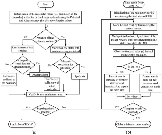
Figure 2.
Flow chart for the hybrid CRO-PS technique, (a) flow chart for CRO, (b) flow chart for PS.
4.2. Pattern Search (PS) Technique
To further advance the system response and the improvised global search, an additional derivative free heuristic method called pattern search is implemented in the proposed search [30]. Moreover, not only is PS flexible for fine tuning the local minima, but also, it has characteristics of coordinated control with other optimization techniques. It starts its operation with the initial assumption of pattern vectors (i.e., [0, 1], [0, −1], [1, 0], n[−1, 0]) and forms a set of mesh points around the initial points by adding the initial vector , as presented in Figure 3. It evaluates the objective function value () for each mesh point of mesh size 1 to determine the presence of any point with a less than that of . If can be obtained, then it is referred to as the initial point for the next iteration, and the mesh size should be twice the current mesh size. Otherwise, the same process has to be repeated by modifying the mesh size to half of the current size, and the initial point remains unaltered for the subsequent iteration. Again, the same process is repeated until the termination criteria is satisfied.
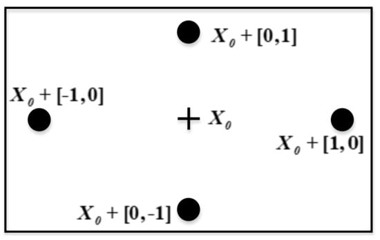
Figure 3.
Formulation of mesh points in PS considering .
4.3. Motivation for Hybridization
As discussed in the previous section, although kinetic energy is the prime factor for the molecular structure to escape the local minima, the same is subtracted and added in the energy buffer so as to decrease the gradually. So, this will finally converge to a global solution. However, during the process, there may be a chance that the solution becomes trapped in local minima. Hence, we introduced PS in the proposed scheme where the final state of CRO is regarded as the initial parameter for PS. Here, PS methods try to find new possible solution with a yet better value around the initial point. PS focuses on set of pattern vectors to obtain the mesh point, as discussed. However, it is not guaranteed to generate a better solution. Hence, searching around the mesh size makes sure that every new possible solution point yields a better solution for each iteration. Thus, the performance of the CRO technique can be further improved with the inclusion of a PS technique in it, as presented in Figure 2. Table 1 presents the characteristics of the considered methods in terms of execution time and memory requirement. The hybrid optimization algorithm needs more time and memory to execute the operation. Table 2 represents the performance of hybrid CRO and PS (hCRO-PS) with various extensive benchmark functions (i.e., constrained and unconstrained functions). The convergence graph of hCRO-PS is shown in Figure 4 and is obtained for a multi-source system subjected to load variation. It can be inferred from Table 2 that hCRO-PS has authority over other optimization algorithms such as CRO and PS.

Table 1.
Technical characteristics of the developed method.
Table 2.
Performance testing of proposed hCRO-PS with constrained and unconstrained benchmark functions.
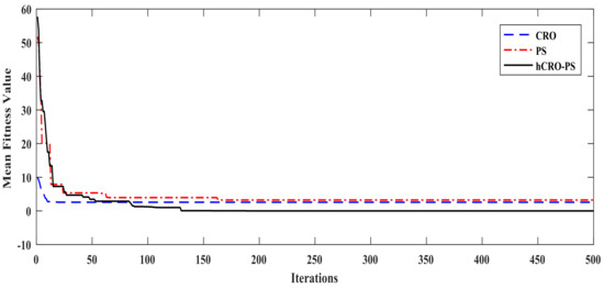
Figure 4.
Convergence graph of the power system tuned by different optimization techniques.
As per the free lunch theorem, it is difficult to claim that certain algorithms perform well for all sets of problems in various fields. In this work, upon the application of the CRO/PS algorithm individually for 500 iterations to tune the parameters of the multi-source system, they are not able reach zero. This may be due to the high complexity of the system and contradictory performance parameters. While we try to reduce the overshoot, the rise time is bound to increase, but to obtain faster settling of the system post disturbance, the rise time should be as small as possible. So, in this process of tuning, both overshoot and settling time are contradictory performance parameters and should be maintained at optimum values rather than minimum values. Thus, the CRO and PS algorithms are combined to formulate hCRO-PS, which successfully handles the complexity of the system while maintaining good convergence characteristics.
5. Controller Formation (PDN-FOPI)
As the complication of the system dynamics grows, an effective controller is needed which has the capability to maintain a stable operating condition and is able to counter any disturbance in a proactive way [15]. The suggested controller is a combination of a PDN controller with a fractional-order PI controller in cascade modes. The expression of the transfer function of the PDN controller is shown in (16).
The structure of the proposed controller is presented in Figure 5. The PD controller generally offers faster set point tracking than the other conventional controllers such as PID controllers. Apart from this design, if an integral mode is added, then the closed-loop response somehow slows down. The controller basically adds zero in the system, which adds a positive angle to the system (moves the root-locus to the left), or in the frequency-domain, it introduces phase-lead to the system (increases the phase margin) so that the system remains in a stable zone. It may be noted that a PD controller might suffer from serious impulsive spikes in its control output due to a step change in the set point, as well as being vulnerable to measurement noise and not realizable for real-time implementation [16]. Hence, to overcome this situation, a first-order lag filter (n) is often augmented with PD controllers, which attenuates high-frequency measurement noise. To further improve the system dynamics, the proposed controller is cascaded with a fractional-order PI controller.
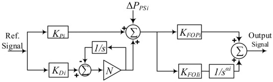
Figure 5.
Block diagram for the proposed controller structure.
With use of fractional calculus, conventional integration and differentiation can be extended to any random real number [14]. One way of representing ordinary calculus is fractional calculus. There are various way to describe fractional calculus such as Grünwald–Letnikov, Riemann–Liouville (RL), and Caputo definitions. Using the R-L criteria, a fractional derivative can be defined by following (17), and lies between n and n − 1. Euler’s gamma function is denoted by ), in which n is the integer. Similarly, the fractional integer can also be expressed as shown in (18), which represents the fractional operator.
If we take the Laplace transform of (17), then (19) is derived.
in which represents the Laplace transform with . Therefore, deduced expression is described in the fractional derivative by differential equations, which can be represented as the fractional order of s if the zero initial condition is presumed. The problem with this type of transfer function is that it contains an infinite number of poles and zeros. Hence, some approximations have to made on which both the fractional-order derivative and integrator lie on a predefined frequency range. There are several approximation techniques available such as Commande Robuste d’Ordre Non-Entier (CRONE), Carlson, Matsuda, high-frequency continued fraction approximation etc. This paper uses the CRONE approximation technique to approximate the equation, and it is depicted in (20).
K denotes the gain term and should be adjustable in such a way that when , the gain is 0 dB for 1 rad/s. Moreover, the number of poles (N) and zero (Z) are already pre-decided. Smaller values of N result in simple approximation but cause ripples in both phase and gain behavior. Although a high value of N decreases the ripple from the system behavior, it makes the approximation too complex. For evaluating the frequency of the pole and zero, Equations (21) to (25) are used.
If the value of v is negative, then the behavior of the poles and zero will interchanged i.e., and so on. From Equations (21) to (25), it can be observed that there is an equal no. of poles and zeros present, and its logarithmic frequencies are equidistant in the range of [, ]. The simple way of representinf a fractional-order PI controller is , and the transfer function is defined as:
Motivation for Cascaded Controller
With the expansion of the test system and integration of non-conventional sources (i.e., wind power plants and PEVs), the objective of maintaining system stability is an essential task. Hence, to fulfil the above objective, a cascaded controller is proposed with optimum numbers of PDN and FOPI controllers. The cascaded controller is designed carefully by keeping the optimum features of PDN and FOPI controllers, as shown in Figure 6.
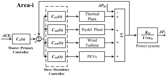
Figure 6.
Block diagram model for arrangement of controller in the multi-source system.
Here, is the slave/secondary controller and is termed as , , , and for thermal, hydro, wind and PEVs, respectively, whereas master/primary controller monitors the total area, and the complete configuration of the controller is projected in Figure 6 for better understanding of the derived Equations (27) and (28). The synchronized action of master and secondary controllers sets up the cascaded PDN-FOPI controller. takes signal as input and produces a corresponding control action. The secondary controllers intakes the resultant signal of the inner process output and signal from . Here, the disturbance signal is for which the stability of the system is to be analyzed.
In a traditional controller structure, two individual controllers are required to control each plant in the system for stable operation. However, this results higher number of controllers (i.e., eight units for each area). This in turn would raise the number of controller parameters and thus the computation time. In addition, the system complexity would increase drastically for the multi-source test system. To overcome these issues, a cascaded controller is considered. Here, four slave loops are considered for four distinct power plants in each area, and a master loop is formed which acts as a supervisor of the whole area. In the slave control loop, an FOPI controller is employed, whereas in the master loop, a PDN controller is engaged. The master loop particularly focuses on improving the system response in the transient state, and the slave loop is dedicated to controlling the challenges raised in the steady state. Thus, the total number of the controllers is reduced to five for each area in the test system, hence decreasing the complexity of the controller implementation and concurrently improving the stability.
6. Result Analysis for Two-Area System
The system in the work considers traditional power sources, renewable power sources, and the PEVs operating simultaneously to maintain the load–demand balance to retain the system stability. The simultaneous operation of sources requires an efficient controller to regulate the system. The process of regulation requires the controller parameters to be tuned adequately. Hence, a hybrid algorithm (hCRO-PS) with improved performance is employed. The tuned values of the controller parameters are limited within the range defined as:
The controller is tested under various operating conditions presented by various cases. The applied % SLP for each area in each test case for the two-area multi-source system is presented in Figure 7.
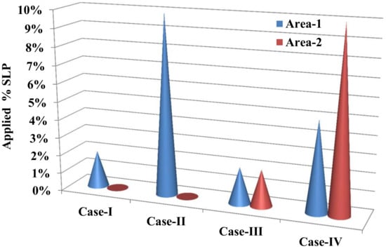
Figure 7.
Test cases for 2-area, multi-source system.
- Case-I: A 2% step load variation occurring only in area-1 and area-2 having no disturbance.
- Case-II: A 10% load variation occurring only in area-1 and area-2 having no disturbance.
- Case-III: A 2% step load variation occurring in both area-1 and 2 simultaneously.
- Case-IV: A 5% and 10% load variation occurring simultaneously in area-1 and area-2.
In Table 3, the Eigen value analysis of the two-area, multi-source system is presented, and it is observed that the damping ratio of the system considering the proposed controller is pretty close to unity, and the system oscillation is negligible. Now, the proposed optimization technique is implemented to obtain the controller parameters for various controllers, as projected in Table 4.
Table 3.
Eigen values (real imag i), corresponding damping ratio, and natural frequency.
Table 4.
Optimized inner loop and outer loop controller parameter.
In Figure 8, the considered load variation is 2% in area-1 only. This shows that although disturbance is induced in area-1, variation in frequency is observed for . In the PID controller, obtaining a optimal balance between integral action and derivative action sometimes leads to an undesirable response. The cascaded controller divides the action into two parts: the master controller (PDN) performs derivative action, and the secondary controller performs integral action. In PIDN, the performance is improved as compared to PID, and further improvement is obtained by applying FOPI. Finally, a better response is obtained with PDN-FOPI as compared to PID, PIDN, and FOPI. It can be observed that the PID and PIDN controllers can achieve good results but provide a low damping factor, resulting in a response which has trivial oscillation (PID) or severe oscillation (PIDN), whereas the FOPI controller successfully suppresses oscillation due to low damping in previous controllers. So, in the work to further improve the system performance, a cascaded controller PDN-FOPI is designed and applied. In Figure 9, Figure 10 and Figure 11, the variation in frequency for a load change described in Case II, III, and IV, respectively, is shown. Similar to the observation of Case I the proposed cascaded controller scheme displays better system performance as compared to the other considered controllers. The operational success of the proposed cascaded controller is clear from the mathematical analysis in Table 5 and the comparison made with the PI-PD controller tuned by Modified Grey Wolf Optimization (MGWO) proposed by [15].
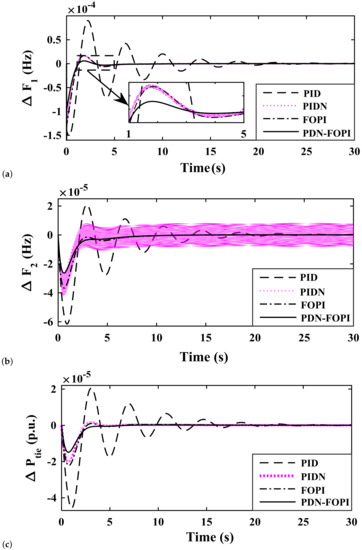
Figure 8.
Study of system response parameters by application of various controllers with a load variation as in Case I (a) Deviation in Frequency of area-1; (b) Deviation in Frequency of area-2; (c) Deviation in Tie-line power.
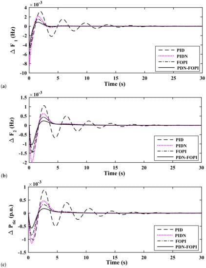
Figure 9.
Study of system response parameters by application of various controllers with a load variation as in Case II (a) Deviation in Frequency of area-1; (b) Deviation in Frequency of area-2; (c) Deviation in Tie-line power.
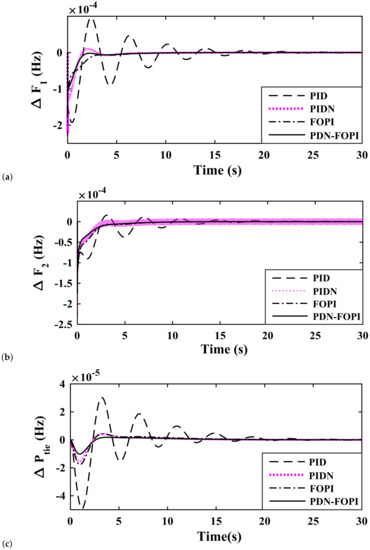
Figure 10.
Study of system response parameters by application of various controllers with a load variation as in Case III (a) Deviation in Frequency of area-1; (b) Deviation in Frequency of area-2; (c) Deviation in Tie-line power.
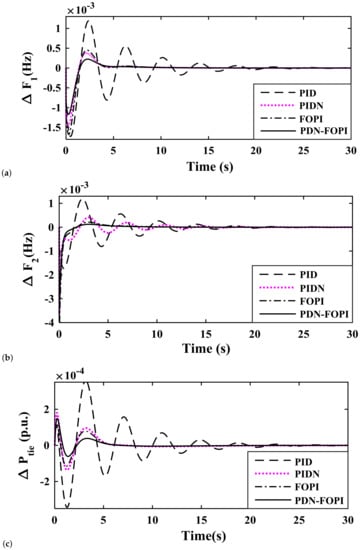
Figure 11.
Study of system response parameters by application of various controllers with a load variation as in Case IV (a) Deviation in Frequency of area-1; (b) Deviation in Frequency of area-2; (c) Deviation in Tie-line power.
Table 5.
Various performance parameter values for the 2-area system analysis under various operating conditions presented by different cases.
Further, the effect of PEVs in different areas is studied to make an efficient placement of PEV along with the proposed controller structure. In Figure 12, the system responses without PEV, PEV in area-1 only, PEV in area-2 only, and PEV in both the areas are shown. Here, it can be observed that the system is most stable when PEVs are placed in both the areas.
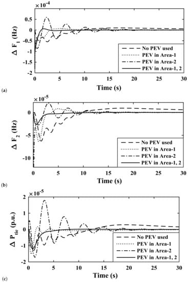
Figure 12.
Studying the effects of implementation of PEV module on various system response parameters (a) Deviation in Frequency of area-1; (b) Deviation in Frequency of area-2; (c) Deviation in Tie-line power.
7. Extension to Three-Area Renewable System
The proposed controller is also verified with use of PEV fleets and several non-linearities (GDB, GRC and BD) in the three-area system. The network configuration of the three-area system is shown in Figure 13, and parameters are provided in Appendix A. Figure 13a shows the block configuration of the three-area system with tie lines, Figure 13b shows the detailed interconnection between these areas, and Figure 13c shows the internal transfer function model of the ith area. Here, PEVs are used extensively for the analysis of a realistic three-area system. The performance is verified based on the deviations in area frequency and power exchange under diverse load perturbation in all of the areas. The effectiveness of the system with the proposed arrangement is paralleled to an analogous work as in [16] with the suggested configuration and some frequently referred controllers, such as PIDF, 2DOFPID, and FOPID, for better understanding of the effectiveness of the large power system to deal with load perturbations.
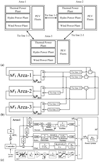
Figure 13.
(a) Block diagram model for multi-source, three-area system with PEVs. (b) Structure of interconnected three-area system. (c) Detailed transfer function model for each area.
8. Result and Analysis for the Three-Area Renewable System
The three-area system discussed in Figure 11 is tested for stability through Eigen value analysis. A total of 53 Eigen values are obtained for the system, of which some significant values are , , , , and . The analysis performed suggests the following regarding the system stability:
- 1.
- The maximum and minimum damping ratios are 1 and 0.9615, respectively. Thus, a very high damping ratio is observed. So, the system would drive back to stability at a faster rate after being subjected to any load perturbation.
- 2.
- The natural frequency variation in the system is observed to be pretty low (i.e., a maximum of 0.012 and a minimum of 0). The oscillation at the transient state would be limited, leading the system to remain in the stable operating zone when subjected to any load perturbation.
The extended work further tests the applicability of the proposed cascaded controller tuned by the hCRO-PS. The system size increases as the scheme becomes more economical as compared to the traditional controller schemes. The controller parameters are in the same range as those of the two-area system. A wide range of load perturbations are applied to test the system performance, which is shown in Figure 14. The applied % SLP for each area in each test case for the three-area, multi-source system is presented in Figure 14.
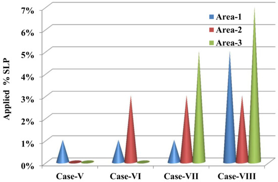
Figure 14.
Test cases for three-area multi-source system.
- Case V: A 1% load variation in area-1, with the other two areas having steady loads.
- Case VI: A 1% and 3% load variation in area-1 and area-2 only.
- Case VII: A 1% and 3% load variation in area-1 and area-2, with area-3 having 5% load perturbations.
- Case VIII: A 5% load variation in area-1 and a 3% load variation in area-2, with area-3 having 7% load perturbations.
- Case IX: Case IX: A dynamic load variation of −5% at 0 s, +5% at 35 s, +5% at 50 s, −8% at 60 s, n+5% at 100 s is applied to the system.
The application of the hCROPS algorithm yields the controller parameter values as in Table 6 for controllers such as PID, PIDN, FOPID, and PDN-FOPI, and are tested on the system. The frequency deviation (i.e., , , n) in each area and tie-line power , , following the application of load deviation described in Case V is projected in Figure 15. Among the considered controllers, the proposed PDN-FOPI controller damps down the oscillation at the earliest time. The unusual response of the other controllers is majorly due to the complexity of the system and applied disturbance. In Figure 16, system responses for the four above-mentioned cases (i.e., Case V, Case VI, Case VII, and Case VIII) are presented. In Table 7 the performance of the proposed controller is compared to that of [16] to present the improvements made in the proposed work. It is observed from Table 7 and Figure 16 that for all four test cases, the proposed controller scheme produces a stable response and is able to damp down the oscillation produced due to load perturbation. The effect of PEVs’ placement in different areas is tested, and the system responses for the various combinations are presented in Figure 17. The simultaneous placement of PEVs in all areas produces a more stable response, as observed from Figure 17. The dynamic load change applied to test the system response is presented in Figure 18. In Figure 19, the system response for the three-area, multi-source system considering the dynamic load change in Case IX is presented. The stability of the system improves significantly when the PEVs are considered. Finally, the effects of variation in SOC are discussed and presented in Figure 20. From Figure 20, it can be observed that variation in SOC can be effectively handled by the designed system in the presence of the proposed controller.
Table 6.
Controller parameter values for the three-area system tuned by hCRO-PS.
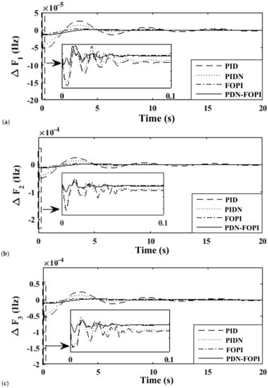
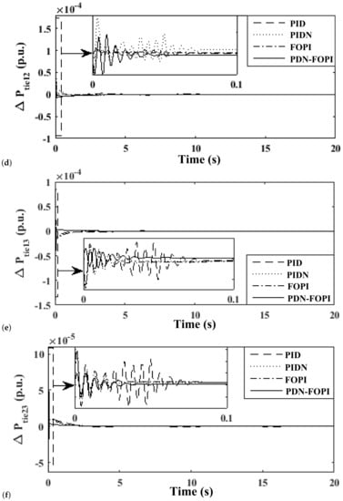
Figure 15.
Study of system response parameters for various controllers with a load variation as in Case V Deviation in Frequency of (a) area-1; (b) area-2; (c) area-3; Deviation in Tie-line power (d) area-1,2; (e) area-1,3; (f) area-2,3.
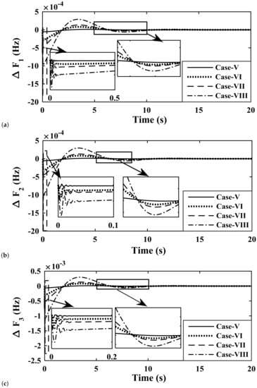
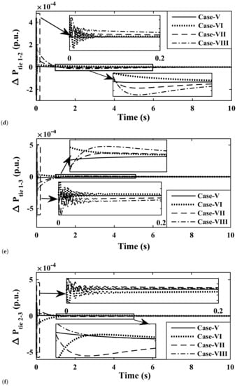
Figure 16.
Study of system response parameters for various controllers with a load variation as in Case V, VI, VII, and VIII Deviation in Frequency of (a) area-1; (b) area-2; (c) area-3; Deviation in Tie-line power (d) area-1,2; (e) area-1,3; (f) area-2,3.
Table 7.
Various performance parameter values for the three-area system analysis under various operating conditions.
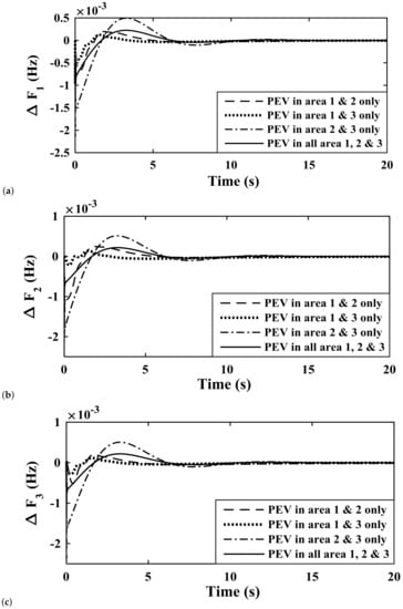
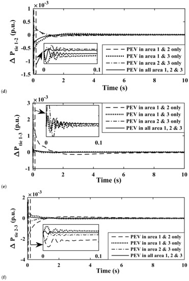
Figure 17.
Studying the effects of implementation of PEV module in different areas on various system response parameters Deviation in Frequency of (a) area-1; (b) area-2; (c) area-3; Deviation in Tie-line power (d) area-1,2; (e) area-1,3; (f) area-2,3.
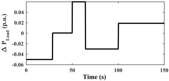
Figure 18.
Dynamic load variation discussed in Case IX applied to multi-source, three-area system.
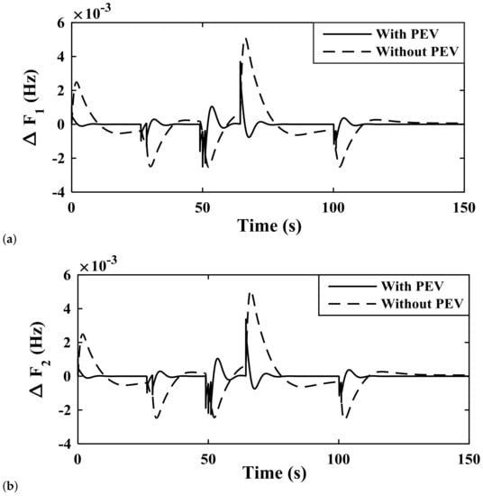
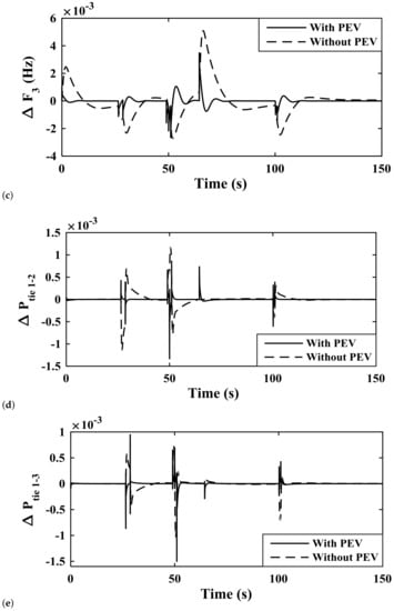
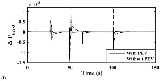
Figure 19.
Study of system response parameters with and without PEV module in the three-area system with a load variation as in Case IX Deviation in Frequency of (a) area-1; (b) area-2; (c) area-3; Deviation in Tie-line power (d) area-1,2; (e) area-1,3; (f) area-2,3.
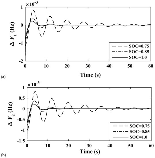
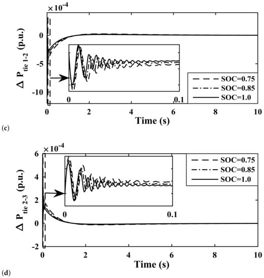
Figure 20.
Studying the effects of variation of state of charge (SOC) of PEV module on various system response parameters Deviation in Frequency of (a) area-1; (b) area-2; Deviation in Tie-line power (c) area-1,2; (d) area-2,3.
9. Conclusions
The testing of a renewable-energy-based AGC system with fleets of PEVs regulated by the proposed cascaded PDN-FOPI controller is proven to be stable in both two- and three-area, multi-source systems. The damping ratio lies in the stable range, i.e., [0 −1] during Eigen value analysis, and the frequency of oscillation is also low.
- 1.
- 2.
- The proposed cascaded PDN-FOPI controller is effective in eliminating any deviation in frequency and tie-line power caused by generation–demand imbalance and under varying SOC states, as seen in Table 5 and Table 6 and Figure 8, Figure 9, Figure 10, Figure 11, Figure 12, Figure 15, Figure 16, Figure 17, Figure 18, Figure 19 and Figure 20.
- 3.
- The effects on the system dynamics due to the placement of PEVs shows that if all areas have similar loading, then maximum stability can be achieved.
- 4.
- The variation in SOC does affect the system performance, but the proposed cascaded PDN-FOPI controller is able to maintain the stability of the system.
Renewable power sources and PEVs come with environmental constraints and their own limitations, such as PV power curtailment, and wind power de-loading. Vehicle-to-grid (V2G) and grid-to-vehicle (G2V) need further attention with the proposed control approach. Furthermore, The use of big data and other technologies in low-inertia grids to assess frequency stability is an important aspect that should be investigated in future research.
Author Contributions
A.B. & S.S.P.: Conceptualization, Methodology, Software, Writing—original draft, Writing— review & editing, Validation. S.G., U.S. & T.K.P.: Conceptualization, Methodology, Writing—review & editing, Supervision, Visualization. M.H.A. & S.M.: Writing—review & editing, Visualization. All authors have read and agreed to the published version of the manuscript.
Funding
This research received no external funding.
Institutional Review Board Statement
Not applicable.
Informed Consent Statement
Not applicable.
Data Availability Statement
Not applicable.
Conflicts of Interest
The authors declare no conflict of interest.
Abbreviations
The following abbreviations are used in this manuscript:
| PEV | Plug-in electrical Vehicle |
| FO | Fractional Order |
| AGC | Automatic Generation Control |
| FOPID | Fractional-Order Proportional Integral Derivative |
| PDN | Proportional Derivative With Filter |
| SLP | Step Load Perturbation |
| FOPI | Fractional-Order Proportional Integral |
| PFC | Primary Frequency Control |
| hCRO-PS | Hybrid Chemical Reaction Optimization with Pattern Search |
| LFC | Load Frequency Control |
| SOC | State Of Charge |
| ITAE | Integral Of Time Multiplied by Absolute Error |
| GRC | Generation Rate Constraint |
| IAE | Integral of Absolute Error |
| GDB | Governor Dead Band |
| ITSE | Integral of Time Multiplied by Square Error |
| BD | Boiler Dynamics |
| ISE | Integral of Square Error |
| EVs | Electric Vehicles |
| ISTSE | Integral Square Time Multiplied by Square Error |
| V2G | Vehicle to Grid |
| AHP | Analytic Hierarchy Process |
| I | Integral |
| CRO | Chemical Reaction Optimization |
| PI | Proportional Integral |
| PS | Pattern search |
| PIDN | Proportional Integral Derivative With Filter |
| RL | Riemann–Liouville |
| DOF | Degree of Freedom |
| MGWO | Modified Grey Wolf Optimization |
| IO | Integer Order |
| Variable/Parameter | |
| Transfer function of wind | |
| Time constant | |
| Feed Forward Gain | |
| Upper Limit | |
| Lower Limit | |
| Aggregate Droop Characteristics | |
| EVs gain | |
| EVs time constant | |
| Maximum derived power | |
| Minimum derived power | |
| Number of electric vehicles | |
| Peak Over Shoot of deviation in frequency in area-1 and 2 | |
| Peak Over Shoot of deviation in power in tie line | |
| Settling time of frequency deviation of area-1 and 2 | |
| Settling time of deviation in power in tie line | |
| Frequency of area-1 | |
| Frequency of area-2 | |
| Associated gains of respective cost function | |
| Represents the relative significance of ith with respect to jth parameter | |
| Energy State | |
| Transfer function of PDN controller | |
| Proportional gain | |
| Derivative gain | |
| N | First-order lag filter |
Appendix A
| Variable | Value | Variable | Value | Variable | Value |
| F | 60 Hz | s | |||
| p.u. | s | ||||
| 120 | s | ||||
| 20 s | 10 s | Hz/p.u. | |||
| p.u. | 1 s | ||||
| 1 | |||||
| s | 2000 |
References
- Elgerd, O.I. Electric Energy Systems Theory an Introduction; McGraw-Hill Book Company: New York, NY, USA, 2000. [Google Scholar]
- Haes Alhelou, H.; Hamedani-Golshan, M.E.; Njenda, T.C.; Siano, P. A survey on power system blackout and cascading events: Research motivations and challenges. Energies 2019, 12, 682. [Google Scholar] [CrossRef]
- Bevrani, H. Robust Power System Frequency Control; Springer: New York, NY, USA, 2009; p. 85. [Google Scholar]
- Elgerd, O.I.; Fosha, C.E. Optimum megawatt-frequency control of multiarea electric energy systems. IEEE Trans. Power Appar. Syst. 1970, 4, 556–563. [Google Scholar] [CrossRef]
- Nanda, J.; Mangla, A.; Suri, S. Some new findings on automatic generation control of an interconnected hydrothermal system with conventional controllers. IEEE Trans. Energy Convers. 2006, 21, 187–194. [Google Scholar] [CrossRef]
- Nanda, J.; Mishra, S.; Saikia, L. Maiden application of bacterial foraging-based optimization technique in multiarea automatic generation control. IEEE Trans. Power Syst. 2009, 24, 602–609. [Google Scholar] [CrossRef]
- Gozde, H.; Taplamacioglu, M.C. Automatic generation control application with craziness based particle swarm optimization in a thermal power system. Int. J. Electr. Power Energy Syst. 2011, 33, 8–16. [Google Scholar] [CrossRef]
- Sahu, R.K.; Panda, S.; Padhan, S. A hybrid firefly algorithm and pattern search technique for automatic generation control of multi area power systems. Int. J. Electr. Power Energy Syst. 2015, 64, 9–23. [Google Scholar] [CrossRef]
- Bhatt, P.; Roy, R.; Ghoshal, S.P. GA/particle swarm intelligence based optimization of two specific varieties of controller devices applied to two-area multi-units automatic generation control. Int. J. Electr. Power Energy Syst. 2010, 32, 299–310. [Google Scholar] [CrossRef]
- Saikia, L.C.; Nanda, J.; Mishra, S. Performance comparison of several classical controllers in AGC for multi-area interconnected thermal system. Int. J. Electr. Power Energy Syst. 2011, 33, 394–401. [Google Scholar] [CrossRef]
- Sopian, K.; Fudholi, A.; Ruslan, M.H.; Sulaiman, M.Y.; Alghoul, M.A.; Yahya, M.; Amin, N.; Haw, L.C.; Zaharim, A. Optimization of a stand-alone wind/PV hybrid system to provide electricity for a household in Malaysia. In Proceedings of the 4th IASME/WSEAS International Conference on Energy & Environment, Algarve, Portugal, 11–13 June 2009; pp. 435–438. [Google Scholar]
- Kadri, R.; Gaubert, J.-P.; Champenois, G. An improved maximum power point tracking for photovoltaic grid-connected inverter based on voltage-oriented control. IEEE Trans. Ind. Electron. 2011, 58, 66–75. [Google Scholar] [CrossRef]
- Kartalidis, A.; Atsonios, K.; Nikolopoulos, N. Enhancing the self-resilience of high-renewable energy sources, interconnected islanding areas through innovative energy production, storage, and management technologies: Grid simulations and energy assessment. Int. J. Energy Res. 2021, 45, 13591–13615. [Google Scholar] [CrossRef]
- Debbarma, S.; Dutta, A. Utilizing electric vehicles for LFC in restructured power systems using fractional order controller. IEEE Trans. Smart Grid 2017, 8, 2554–2564. [Google Scholar] [CrossRef]
- Padhy, S.; Panda, S.; Mahapatra, S. A modified GWO technique based cascade PI-PD controller for AGC of power systems in presence of Plug in Electric Vehicles. Eng. Sci. Technol. Int. J. 2017, 20, 427–442. [Google Scholar] [CrossRef]
- Saha, A.; Saikia, L.C. Renewable energy source-based multiarea AGC system with integration of EV utilizing cascade controller considering time delay. Int. Trans. Electr. Energy Syst. 2019, 29, e2646. [Google Scholar] [CrossRef]
- Fotopoulou, M.; Rakopoulos, D.; Blanas, O. Day Ahead Optimal Dispatch Schedule in a Smart Grid Containing Distributed Energy Resources and Electric Vehicles. Sensors 2021, 21, 7295. [Google Scholar] [CrossRef]
- Li, T.; Tao, S.; He, K.; Lu, M.; Xie, B.; Yang, B.; Sun, Y. V2G multi-objective dispatching optimization strategy based on user behavior model. Front. Energy Res. 2021, 494. [Google Scholar] [CrossRef]
- Morsali, J.; Zare, K.; Hagh, M.T. Applying fractional order PID to design TCSC-based damping controller in coordination with automatic generation control of interconnected multi-source power system. Eng. Sci. Technol. Int. J. 2017, 20, 1–17. [Google Scholar] [CrossRef]
- Ismayil, C.; Sreerama, K.R.; Sindhu, T.K. Automatic Generation Control of Single Area Thermal Power System with Fractional Order PID (PIλDμ) Controllers. IFAC Proc. Vol. 2014, 47, 552–557. [Google Scholar] [CrossRef]
- Kumar, M.R.; Ghosh, S.; Das, S. A hybrid optimization-based approach for parameter estimation and investigation of fractional dynamics in ultracapacitors. Circuits Syst. Signal Process. 2016, 35, 1949–1971. [Google Scholar] [CrossRef]
- Chang, W.-D.; Chen, C.-Y. PID controller design for MIMO processes using improved particle swarm optimization. Circuits Syst. Signal Process. 2014, 33, 1473–1490. [Google Scholar] [CrossRef]
- Sundararaju, N.; Vinayagam, A.; Veerasamy, V.; Subramaniam, G. A Chaotic Search-Based Hybrid Optimization Technique for Automatic Load Frequency Control of a Renewable Energy Integrated Power System. Sustainability 2022, 14, 5668. [Google Scholar] [CrossRef]
- Alam, M.S.; Al-Ismail, F.S.; Abido, M.A. PV/Wind-Integrated Low-Inertia System Frequency Control: PSO-Optimized Fractional-Order PI-Based SMES Approach. Sustainability 2021, 13, 7622. [Google Scholar] [CrossRef]
- Das, D.; Aditya, S.K.; Kothari, D.P. Dynamics of diesel and wind turbine generators on an isolated power system. Int. J. Electr. Power Energy Syst. 1999, 21, 183–189. [Google Scholar] [CrossRef]
- Khudhair, M.; Ragab, M.; AboRas, K.M.; Abbasy, N.H. Robust Control of Frequency Variations for a Multi-Area Power System in Smart Grid Using a Newly Wild Horse Optimized Combination of PIDD2 and PD Controllers. Sustainability 2022, 14, 8223. [Google Scholar] [CrossRef]
- Shinners, S.M. Modern Control System Theory and Design; John Wiley & Sons, Inc.: New York, NY, USA, 1998; ISBN 0471249068. [Google Scholar]
- Ghatak, S.; Rup, S.; Majhi, B.; Swamy, M.N.S. HSAJAYA: An improved optimization scheme for consumer surveillance video synopsis generation. IEEE Trans. Consum. Electron. 2020, 66, 144–152. [Google Scholar] [CrossRef]
- Lam, A.Y.S.; Li, V.O.K. Chemical-reaction-inspired metaheuristic for optimization. IEEE Trans. Evol. Comput. 2010, 14, 381–399. [Google Scholar] [CrossRef]
- Dolan, E.D.; Lewis, R.M.; Torczon, V. On the local convergence of pattern search. SIAM J. Optim. 2003, 14, 567–583. [Google Scholar] [CrossRef]
Publisher’s Note: MDPI stays neutral with regard to jurisdictional claims in published maps and institutional affiliations. |
© 2022 by the authors. Licensee MDPI, Basel, Switzerland. This article is an open access article distributed under the terms and conditions of the Creative Commons Attribution (CC BY) license (https://creativecommons.org/licenses/by/4.0/).