Automatic Selection of Temperature Variables for Short-Term Load Forecasting

Abstract

Due to the infeasibility of large-scale electrical energy storage, electricity is generated and consumed simultaneously. Therefore, electricity entities need consumption forecasting systems to plan operations and manage supplies. In addition, accurate predictions allow renewable energies on electrical grids to be managed, thereby reducing greenhouse gas emissions. Temperature affects electricity consumption through air conditioning and heating equipment, although it is the consumer’s behavior that determines specifically to what extent. This work proposes an automatic method of processing and selecting variables, with a two-fold objective: improving both the accuracy and the interpretability of the overall forecasting system. The procedure has been tested by the predictive system of the Spanish electricity operator (Red Eléctrica de España) with regard to peninsular demand. During the test period, the forecasting error was consistently reduced for the forecasting horizon, with an improvement of 0.16% in MAPE and 59.71 MWh in RMSE. The new way of working with temperatures is interpretable, since they separate the effect of temperature according to location and time. It has been observed that heat has a greater influence than the cold. In addition, on hot days, the temperature of the second previous day has a greater influence than the previous one, while the opposite occurs on cold days.

1. Introduction

On a national scale, it is not feasible to store energy on electrical grids before transmitting it to consumers. Therefore, electrical operators maintain a real-time balance between produced and consumed energy. To maintain this balance, it is necessary to forecast the future electric load. Forecasting is necessary in the very short-term for the control of generators, and in the short and medium term for resource supply and operations planning. In addition, long-term forecasting is required for the construction and maintenance of facilities. This paper focuses on short-term load forecasting (STLF), ranging from hours to several days in advance, being necessary for energy and the economic management in electrical companies, such as marketers, demand aggregators, generators, etc.

Predicting demand accurately is crucial to reliably operating power generation, transmission and distribution. Making decisions based on inaccurate predictions can lead to additional costs, breakdowns and even blackouts. Furthermore, accurate forecasts allow better management of renewable energies, so load forecasting can help reduce greenhouse gas emissions indirectly.

The electrical load depends on many variables, such as time of the day, temperature, day of the week or industrial activity, and it even has a random component, so there is always some error. In addition, these variables show interaction among them. For example, temperature has a greater effect during the afternoon than during early morning, since air conditioning units are generally less used while people sleep. This paper deals specifically with temperature variables and how they can be automatically selected and processed to properly capture their effect on load and, therefore, forecast electrical load more accurately.

1.1. Literature Review

Over the last decades, many works have been published developing predictive models, and so a wide variety of models have been built. Some of them are based on statistical models, such as ARIMA and the Hidden Markov Model [1], the autoregressive [2,3], exponential smoothing grey model [4], the exponential smoothing model [5], or a single ARIMA [6]. Other models are based on machine learning, such as the radial basis function neural network [7], fuzzy interaction regression [8] or convolutional neural network with long short-term memory [9]. There are also hybrid forecasting systems that combine artificial intelligence with statistical techniques like ARIMA and support vector machine [10], state-space models combined with a neural network [11] or multivariable regression with a long short-term memory network [12].

In recent years, machine learning techniques have received more attention than statisticals. For example, ref. [13] designs a deep-learning model to forecast wind speed and, consequently, electric energy generation; a long short-term memory neural network and a convolutional neural network are combined as a core of the forecasting system. A long short-term memory model is used with a hyperparameter adjustment in [14]. Another work [15] employs a neural network to forecast the load of individual families. Convolutional neural networks can extract non-linear features to feed support vector machines as forecasting systems [16]. An artificial neural network is integrated with an evolutionary algorithm to avoid local optima and obtain convergence [17].

The number of forecasting hybrid techniques has also increased recently. As an example, a fuzzy c-means clustering is employed in [18] using a random forest model and a deep neural network. In [19], an exponential smoothing state-space model and an artificial neural network are combined. The system from [20] combines a SARIMAX with a long-short term memory network to obtain a better forecasting performance.

During the last years, smart grids received more attention due to increased access to data through smart meters. For example, ref. [21] employed a multivariable linear regression to forecast trend and a long short-term memory neural network to model nonlinear behavior of an electric load. In [22], k-means clustering is employed to divide data into sets, they are divided into training and test sets, and a convolutional neural network is finally trained and employed to forecast the load. Another example is [23], which evaluates different machine-learning models for smart grids. In [24], a list of methods for low voltage forecasting are also compared, which mainly consist of kernel density estimation, simple seasonal linear regression, and autoregressive and exponential smoothing.

When it comes to predicting demand, selecting and processing exogenous variables may be more important than the mathematical model used. Other previous works have focused on processing temperature data to accurately forecast load. An example to this is the regressive algorithm of [25], which uses the climate data from five previous days in a model. It is updated with similar previous days employing the shortest Euclidean distance. Fuzzification has also been applied to the temperature before using it in a multi-layered LSTM [26]. This allows the model to adapt to temperature changes and improve its performance. The heat island effect has been taken into account by means of satellite images to correct the temperature before using it in an Elman Neural Network [27], also using the temperature of previous days; however, real predictive systems do not usually have satellite data. A predictive system was developed in Nepal [28] with a feed-forward neural network that uses temperature, working days, holidays, time of the day, month, and previous data. Previously, they analyzed the demand/temperature sensitivity and obtained different values for the cold and hot degree days, then the difference between room heating and cooling systems is obtained.

Mentioned works [25,26,27,28] offer a treatment of climatic variables in order to improve accuracy, but leave interpretability on the background or do not mention it. In contrast, other research has focused on the analysis of the relationship between temperature and demand, such as the use of a linear regression model to extract the correlation in Vietnam [29], where it was observed how the relationship varies throughout the year. In Beijing [30], the relationship was analyzed with linear regression using two demand/temperature lines. One of them is used above a temperature threshold value while the other one is used below. This provides two demand-temperature equations depending on whether it is cold or hot. For this, a threshold temperature is established to separate both behaviors; however, the possibility of an intermediate range of temperatures is not contemplated. In the United Kingdom, the effect that cold temperatures have on demand due to the use of heat pumps was studied [31]. This allowed the calculations of demand forecasts for heat pumps according to temperature.

In Spain, a predictive system that uses differentiated temperature and the effects of daylight at each hour of the day was developed in [32]. The model, called “smooth transition regression model with double threshold”, allows for the distinguishing of the demand/temperature sensitivity for periods of economic activity and rest. Therefore, the predictive model also allows analytical conclusions to be drawn, this being its focus. In this paper we work with an interpretable approach to use temperature by linearizing it with three demand-temperature lines. On the contrary, in [32], temperature was preprocessed by means of a third degree polynomial function against logarithmic demand. In addition, our system works with a model for each hour of execution and forecast, which also considers the cycles of economic activity; this data together with the month implicitly considers daylight; there are also 54 variables that define type of day, reinforcing the information about economic activity as well as allowing the types of day to be distinguished.

In the literature there are also works about the automation of STLF. In 1997, a predictive regressive system was programmed for the Irish Electricity Supply Board [33]. The forecasting calculation and the periodic updating of the model are automated, and the STLF system uses backward elimination to discard temperature variables that are not useful and an algorithm to rule out outliers. More presently, an automatic predictive system that updates and uses a specific model, such as the Stochastic Hour Ahead Proportion Analysis Trained by Multivariable Regression, is presented in [34], which includes a graphical user interface.

Currently, automation can go a step further through open-source libraries that automate the process of generating predictive models, which allows building prediction systems without a need for experts. For example, Auto-Sklearn and Python’s TPOT generate machine learning models. They were used to build models that predicted the consumption levels of appliances in a household and of an industrial office building [35].

There is also the possibility of working at an intermediate point of automation using a library of already defined models. This was the case of the creation of an automatic model selection system using a semi-Markov process and a modified hidden Markov chain [36].

1.2. Paper Contributions

According to [37], there is already a large number of STLF models, each one being the best according to the circumstances. Therefore, a new model is not offered in this paper. Instead, a model-independent temperature data preprocessing technique is developed. In the same way, the model used is also not dependent on the temperature preprocessing. All this allows the proposed technique to by applied to any other forecasting engine using temperature information

By applying this processing technique, this paper seeks to improve the STLF system implemented in the Spanish Transmission System Operator, Red Eléctrica de España (REE) (Municipality of Alcobendas, Spain) and developed by the Miguel Hernández University [38]. The system has been operating for more than five years, and during this time REE and the university have been working on improvements [39,40]. The forecasting system is considered as an adequate benchmark for load forecasting in Spain due to its continuous use and enhancement by the Spanish Transmission System Operator (TSO).

To predict the demand of the Spanish peninsula, the previous REE system had temperature data available from 28 meteorological stations, of which five were used. Stations were chosen by expert advice, following subjective criteria of demography and climatological regions of Spain. This implies that the previous system was not built in an automatic and repeatable way, nor did it have an interpretable way of processing temperatures. As a consequence, many coefficients of the autoregressive models had opposite signs to what was expected, compensating for other effects. In addition, there were 30 variables to represent the temperatures of the forecast day and the two previous ones, which, as shown in this paper, is an unnecessary amount.

Three improvements are offered regarding temperature management:

• Final prediction accuracy.
• Variable selection automation.
• Interpretability of variables.

The new approach consists of working with the following new temperature variables:

• Average temperature from chosen stations.
• Temperature averages from previous days.
• Individual temperatures from chosen stations.
• Individual temperatures from previous days.

The new predictive system starts from the same database, however it is capable of automatically determining how many stations to use, which ones to use, and how many previous days should be considered.

This new way of constructing the temperature variables has replaced the one previously used by the predictive system. To test it, it has been trained with the years from 2012 to 2018, after which 2019 was predicted. An execution of the predictive system has been simulated with the same data availability as under normal conditions. In the simulation, the current day and the following nine days were predicted, executing the system in each of the 24 h of the day. Different ways of processing temperatures have been tested, and the best one obtained higher and more consistent accuracy than the old system.

The new way of working with temperatures is more interpretable since it separates the effects of temperature, according to location and time. Based on the zones, lags and training coefficients, the regions that affect demand can be deduced along with their temperature, how many previous days of temperature affect demand, and by how much.

The new predictive system is also intended to be the test subject for future studies of the temperature-demand relationship.

This paper is organized as follows: Section 2 explains the prediction system used to test the processing of temperature data, Section 3 exposes an updated version of the tested system, Section 4 explains the rest of preprocessing methods tested, Section 5 presents the execution of the simulations to test the preprocessing methods, Section 6 shows the simulation results, and Section 7 presents the conclusions. Section Nomenclature shows variable meanings.

2. Previous Forecasting System

This section explains important aspects to bear in mind from the previous REE system. Design details are shown in the previous work [38].

2.1. Data Employed

Temperature data is taken from the State Meteorological Agency, which consists of measurements and forecasts up to nine days in advance of daily temperatures.

The previous predictive system and the proposed modifications use the same variables except for temperature: holiday information and historical electrical load of the Spanish national network. Holiday information was acquired from the official state gazette (BOE), whilst historical load was provided by REE.

Data are classified into three sets according to purpose: training, validation and testing. Training data are used to calculate internal coefficients of predictive models. Some input data are not applied directly to models, but they are pre-processed using coefficients called hyperparameters. Validation data is used to test and correct these hyperparameters after training models. Test data are used to test trained models. The test data set must be independent and not have any matches with other datasets to ensure generalizability.

2.2. Forecasting Models

The REE forecasting system [38] uses two different model types: an exogenous autoregressive model and a group of exogenous autoregressive networks. Both models employ identical inputs to forecast the peninsular load. They use the following inputs in the same way:

• Temperature predictions for current and the next nine days.
• Peninsular load from the previous hour to calculate the forecast.
• Average load of 52 previous weeks.
• Calendar information, which distinguishes different national and regional holidays including Christmas, weekdays, previous and following days after the time change, month of the year and August week.

The output is the forecasted load for an hour of one of the following nine days or the current one. To obtain multiple forecasted hours, multiple models are then trained with their available inputs and expected output.

Both types of models are employed to calculate forecasts. Their individual results are then combined into a weighted average to obtain final predictions for the operator, so two coefficients from zero to one are applied to each forecast. Both coefficients are calculated to minimize the Mean Absolute Percentage Error (MAPE) of the last 30 days. The forecast horizon spans from the current day up to the next ninth day.

Each neural model is made up of ten feed-forward neural networks with feedback. Every neural network generates its own forecast. The highest and lowest values are then discarded and, finally, the average is calculated to obtain the final neural prediction.

Equation (1) represents the autoregressive model.

$$\ln \left(y_t\right)={\displaystyle \sum }_{i=1}^d{c}_{t-i}{\beta }_i+{\displaystyle \sum }_{k=1}^n{X}_{kt}{\Psi }_k+{\epsilon }_t$$

(1)

where y is the time series of forecast load for an hour of the day, t is the day whose demand is forecast, c is the time series of errors made by the model itself (difference between real value and prediction), β is the series of coefficients associated with the errors, d is the number of previous days that are taken into account, X is the exogenous input vector to predict a day t composed of a number k of variables, Ψ are their respective coefficients and ε is a Gaussian random variation with zero mean.

To operate with the natural logarithm instead of the directly forecast load, it is expressed according to (2).

$$y_t=e^{{\epsilon }_t}{e}^{{{\displaystyle \sum }}_{i=1}^d{c}_{t-i} {\beta }_i}{{\displaystyle \prod }}_{k=1}^n{e}^{X_{k t} {\Psi }_k}$$

(2)

In (2) the entire expression is made up of a series of multiplications of e raised to two multiplied elements, so the effect of an exogenous variable can be isolated according to (3). Therefore, each input variable can be interpreted as a load variation proportional to the Euler number (e) raised to the variable by its coefficient.

$$y_t=y_t^{\prime }{e}^{A{\Psi }_a}$$

(3)

Being A any exogenous variable desired to analyze, Ψ_a its respective coefficient and y_t′ the demand without taking said variable into account. That is, variable y_t′ is calculated as shown in (1) or (2) discarding the variable A and its respective coefficient Ψ_a.

The autoregressive model predicts the natural logarithm of the demand in (1) for interpretability reasons. In this way, the demand can be expressed as a series of multiplications in (2) and isolate the influence of the variable to be analyzed in (3), that is, as a multiplication factor for the demand. For example, given a variable A and its respective coefficient Ψ_a, if the result of e^{A Ψa} is 1.05, the variable A increases demand by 5%.

2.3. Use of Temperature

For measurements and forecasts, there exist daily maximum and minimum values. The daily temperature is then represented by the mean of both values.

The old predictive system does not use this average temperature directly, but preprocesses it with a linearization. To do this, two thresholds are first calculated, and they separate temperature into three intervals: cold, hot and warm. Equations (4) and (5) are then applied, resulting in two new variables that indicate the degree of cold and heat.

$$C{D}_z=\left\{\begin{array}{c}0, T_z\ge Th{c}_z\\ Th{c}_z-T_z, T_z<Th{c}_z\end{array}\right.$$

(4)

$$H{D}_z=\left\{\begin{array}{c}0, T_z\le Th{h}_z\\ T_z-Th{h}_z,T_z>Th{h}_z\end{array}\right.$$

(5)

where CD is the cold degree, T is the temperature, Thc_z is the cold threshold for zone z, HD is the heat degree and Thh_z is the heat threshold for zone z. There is then only a pair of thresholds for each zone.

These two thresholds are the hyperparameters used to process temperature. All variables have subscript z because they are specific for each zone.

To calculate thresholds Thc_z and Thh_z for each weather station, the method from the same paper where the forecasting system is explained [38] has been used. The method consists of creating a demand-temperature curve divided into three straight lines (cold, warm and hot), so that the three lines are delimited by the thresholds. Thresholds and line coefficients are then calculated by minimizing the Root Mean Square Error (RMSE) of the triple curve with respect to the real demand. After applying minimization, the thresholds obtained are the results.

The heat degree and cold degree of each region are used as inputs to the prediction system, the selected regions being Zaragoza, Madrid, Biscay, Seville, and Barcelona. In addition, these variables are also used for the temperature data of the previous day and the previous one. There are then a total of 30 variables: five regions for two degree variables for 3 days.

3. Updated Forecasting System

As an alternative benchmark, a modified version of the old REE system has been tested which is called the Updated Forecasting System. It still works with variables CD and HD from (4) and (5), but the difference lies in using a pair of thresholds Thc_z and Thh_z for each hour of each zone z. This method then forecasts load in a similar way to the original system, following the next steps:

Step 1, calculate Thc_z and Thh_z for each hour of each zone, with historical data.

Step 2, calculate CD and HD with temperatures from the training dataset.

Step 3, train models with CD, HD and the rest of inputs, which are not temperature data.

Step 4, calculate CD and HD with temperatures from the test dataset.

Step 5, forecast with CD, HD and the rest of inputs, which are not temperature data.

Although temperatures are daily values, a pair of thresholds is used for each hour of the day. Pairs of thresholds are updated with data from 2011 to 2018; no special days or holidays are considered to minimize the effect of other factors on load. For each hour of the day, a couple of thresholds have been obtained using the demand for that same hour.

When discarding days of the data, they become discontinuous, but this is not an inconvenience, since the procedure to obtain thresholds does not use the autoregressive model, as explained in the previous section.

4. Alternative Processing Methods

This section explains the different alternative methods of temperature processing. All procedures use variables presented from (6) to (14).

$$T{M}_t=\frac{1}{nz}{\displaystyle \sum }_{z=1}^{nz}{T}_{zt}$$

(6)

$$H{N}_t=\left\{\begin{array}{c}0, T{M}_t\le Th{h}_n\\ T{M}_t-Th{h}_n, T{M}_t>Th{h}_n\end{array}\right.$$

(7)

$$C{N}_t=\left\{\begin{array}{c}0, T{M}_t\ge Th{h}_n\\ Th{h}_n-T{M}_t, T{M}_t<Th{h}_n\end{array}\right.$$

(8)

where TM is the time series for the mean national temperature, t is the forecasted day, and T_z is the time series for temperature from zone z. As an example, T_{2 3} represents the temperature during the third day in the second zone. The number of zones is nz, CN is the cold degree time series for the national mean, Thc_n is the cold national threshold, HN is the heat degree time series for the national mean, and Thh_n is the heat national threshold. As in the updated version, there are a few different thresholds depending on the time of the day.

$$P{C}_{nl t}=C{N}_{t-nl}-C{N}_t$$

(9)

$$P{H}_{nl t}=H{N}_{t-nl}-H{N}_t$$

(10)

where PC_l is the previous cold degree time series for nl previous days and PH_l is the previous heat degree time series.

$$I{C}_{z t }=C{D}_{z t }-C{N}_t$$

(11)

$$I{H}_{zt}=H{D}_{zt}-H{N}_t$$

(12)

where IC_z is the individual cold degree difference of zone z and IH_z is the individual heat degree difference of zone z. For example, IC_{2 3} represents the cold degree difference during the third day in the second zone.

$$PI{C}_{z zl t }=C{D}_{z t-zl }-C{N}_{t-zl}$$

(13)

$$PI{H}_{zzlt}=H{D}_{zt-zl}-H{N}_{t-zl}$$

(14)

4.1. Combinatorial Brute Force

This method looks for the best zone and lag combination so that all possible combinations are tested.

4.1.1. Steps

Step 1, individual thresholds. Individual thresholds (Thc_z and Thh_z) are obtained for all available zones.

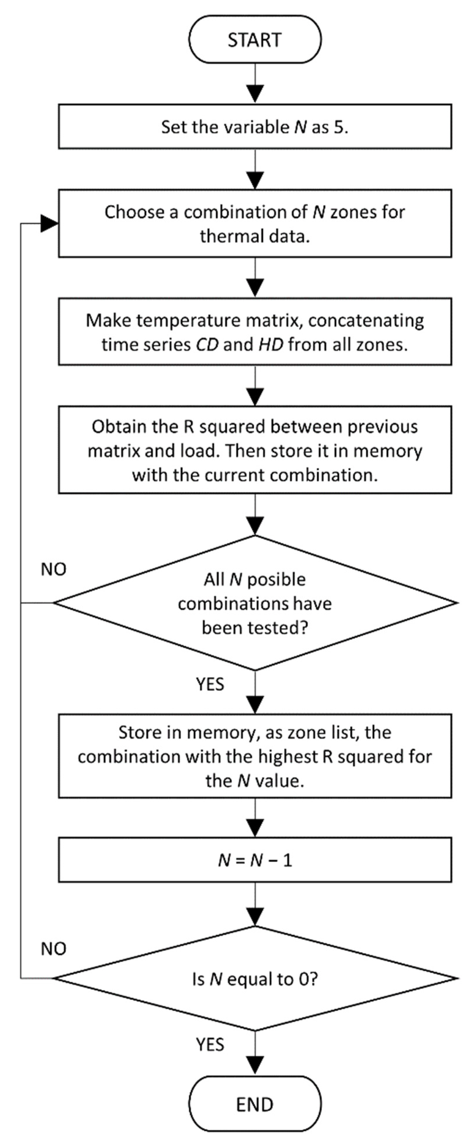
Step 2, number and zone selection. All possible choices that include five zones are tried. For each combination of zones, the R squared for a linear model is calculated between temperature matrix and peninsular demand, this matrix is made up of time series CD_z and HD_z. Next, the combination of zones with the highest R squared is chosen. The whole process is repeated for one, two, three and four zones, so that five zone lists are obtained. This step is summarized in Figure 1.

Step 3, peninsular thresholds. For each zone list, Thc_n and Thh_n are calculated.

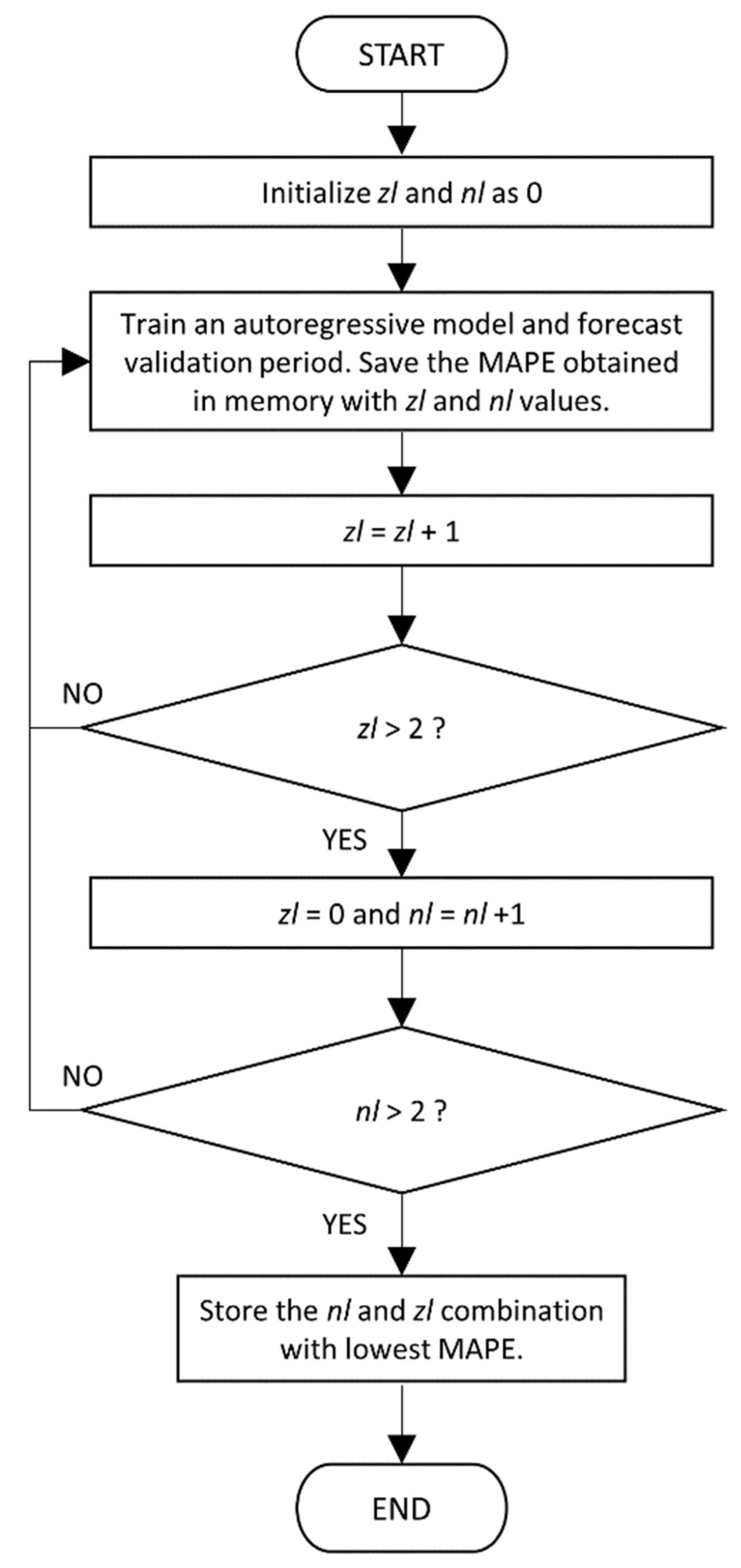
Step 4, peninsular and individual lags. For each list, all possible combinations of individual lags zl for each zone and national nl are tested, which can be 0, 1 or 2. During each iteration, an autoregressive model is trained with all the exogenous variables simulating real training (for the fourth day before, executing at 10:00 a.m. and predicting at 6:00 p.m.). The combination with the lowest MAPE in the validation period is chosen as the result. This step is summarized in Figure 2.

4.1.2. Datasets

For steps 1, 2 and 3, only days that are not holidays or special weekdays are considered, in order to minimize the effect of other factors on demand. Data from 2011 to 2018 have been used.

For step 4, every day from 2011 to 2017 has been used as a training period and data from 2018 have been taken as the validation to calculate error and compare combinations.

4.2. Sequential Brute Force

This algorithm follows the same steps as the combinational one, but it searches for the best thermal zones one by one instead of all possible combinations. To do this, step 2 is changed to the following:

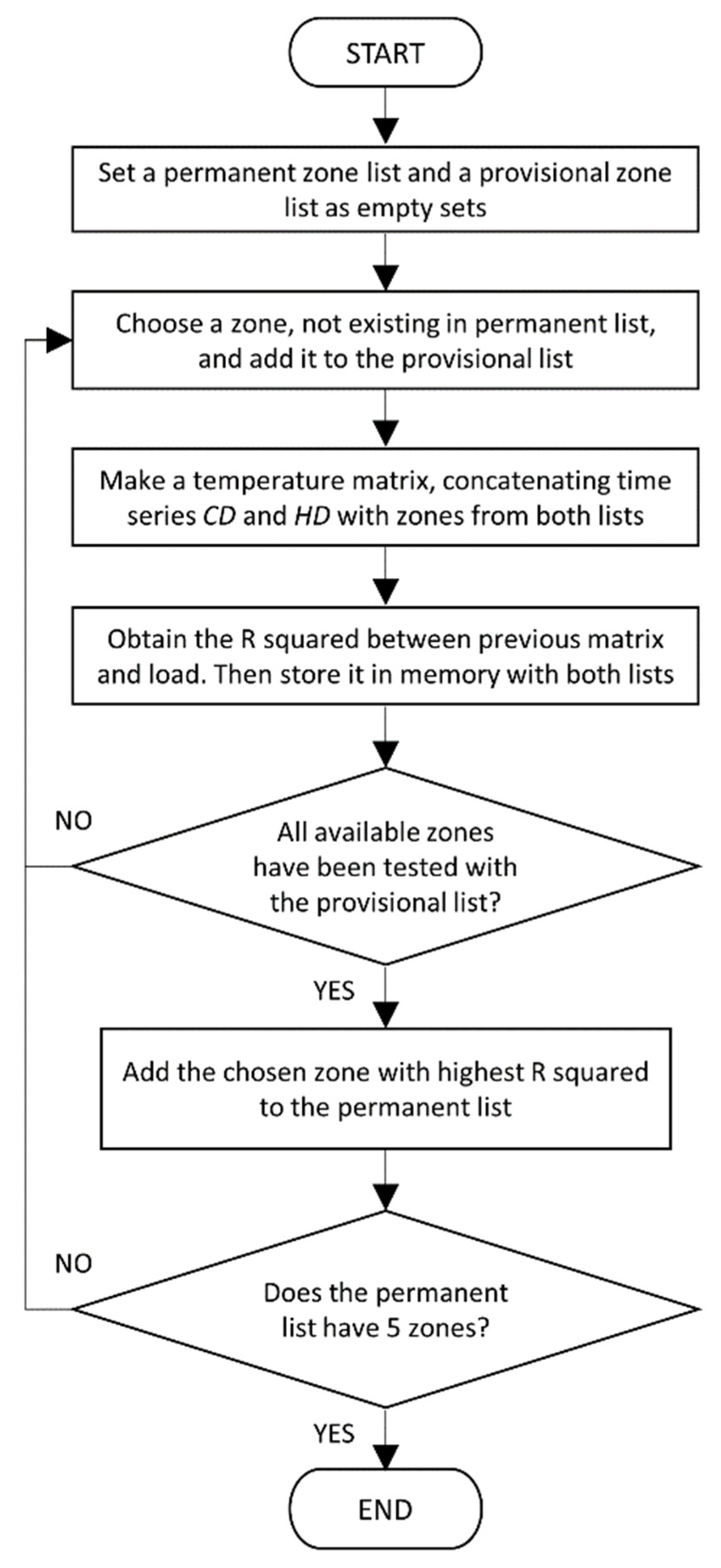
For each zone, the matrix composed with time series CD_z and HD_z is created, obtaining a matrix composed by two time-series. Then, R squared is calculated with respect to load, employing a linear model and the matrix itself; this process is repeated for all the rest of the zones. The first registered zone is the one with the highest squared. After that, the second zone is searched. Then, the R squared is calculated by concatenating the matrix of the first registered zone with each matrix of the other zones. The second registered zone will be the one that offers the best correlation between the load and the concatenated matrices. This loop is repeated up to five times, adding the registered zones one by one to the previous matrices, thus obtaining a list of the five best zones. Since zones were added in correlation order, the list can be shortened to use less zones by removing the last elements. This step is summarized in Figure 3.

4.3. Combinatorial Completeness

This technique follows the same steps and datasets as the Combinatorial Brute Force, but it uses all possible variables to take advantage of all the information. To do this, step 2 only obtains the list of five zones, and step 4 automatically chooses two previous individual days, zl and nl, since it is the maximum possible value.

4.4. Sequential Completeness

This method is also analog to the Sequential Brute Force, with the difference that this method takes advantage of all the information. Therefore, it results as follows:

Step 1, individual thresholds. Individual thresholds (Thc_z and Thh_z) are obtained for all available zones.

Step 2, number and zone selection. For each zone, the matrix composed of time series CD_z and HD_z is created. Then, R squared is calculated with respect to load with a linear model. This process is then repeated for the rest of the zones and, finally, the one that achieves the highest R squared is selected and the first zone is registered. Subsequently, the second zone is searched. The R squared is calculated by concatenating the matrix of the first zone with each one of the others. The second registered zone will be the one that offers the best combination. This process is repeated up to five times, adding the registered zones one by one, thus obtaining a list of the best five zones. This step is also summarized in Figure 3, since it is identical to Sequential Brute Force, but it is explained again to show a general view.

Step 3, peninsular thresholds. Thc_n and Thh_n are calculated for the list of zones obtained.

Step 4, peninsular and individual lags. Two previous individual days, zl and peninsular nl, are chosen since it is the maximum value.

5. Forecasting Simulation

The REE models have been trained and used to forecast 2019 in a simulation with each preprocessing option. The only difference between models is the input temperature variables set, which has been explained in previous sections.

5.1. Training

All models have been trained with data from 2012 to 2018. Seven years of training have been used to ensure that all possible special days are included, offering better accuracy in the process [39].

When training the models, there are two options regarding temperature data. One option is to use only real measurements. The second option uses forecasted values along with measurements, respecting the data availability of real time.

An example of the second option is the case of a model that forecasts the current day and uses the real temperature from the previous day. It would use the temperature forecast as data for the current day and real measurements from the previous day.

If the first training option is used, some weight will be assigned to the temperature variables to deal with precise temperature data. If the second option is used, the temperature data will be based on forecasts, so there will be some error. Consequently, they will have less correlation with the real demand and lower weights will be assigned to them. If a predictive model is trained with measurements only, although it will actually work with predictions, the error induced in the temperature forecasts will affect the accuracy of the load forecast. Therefore, training is executed with the second option for this work. In addition, coefficients of autoregressive models will reflect the temperature-demand correlation.

5.2. Forecasting

The tests of this work have been carried out with Matlab R2020a with Windows 10 Home as operating system on a computer with an Intel Core i7-8700 as CPU and 16 GB RAM.

The year 2019 has been used as the test dataset, so it has been predicted to calculate the errors of all systems. To calculate forecasts, a predictive system execution has been simulated throughout the year, so the current and the following nine days have been forecasted during every hour of the year. Therefore, the 24 hours of the day have been predicted for the whole year every hour since nine days before the forecasted day.

Data availability has been considered. Therefore, during the simulation, data that would be available at each moment has been used. For example, to forecast an hour of the following day, temperature measurements are not used. Instead, temperature forecasts from one day in advance are used. The data employed on this work have been provided by REE and the Spanish State Meteorology Agency (AEMET).

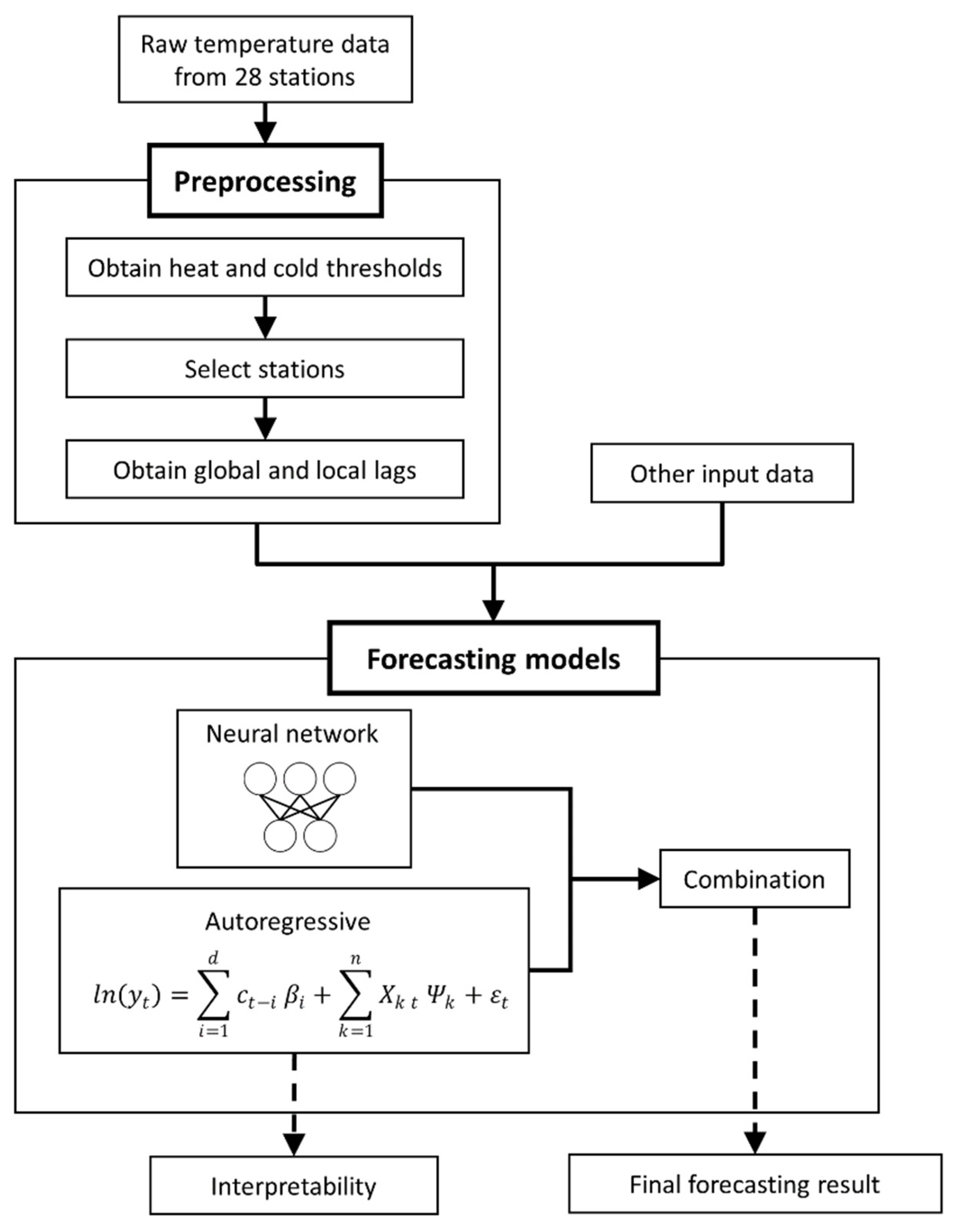
Figure 4 is a summary of the process carried out in this paper to obtain forecasts and analyses.

6. Results

Regardless of temperature processing, a predictive system is made up of autoregressive and neural models, so final forecasts are obtained from the combination of both results. The performance of results (combinatorial) is analyzed to evaluate the usefulness of the system from the point of view of an electrical operator. On the other hand, the performance of the autoregressive approach is analyzed to validate it as an analytical model to study the temperature-demand relationship in the future.

MAPE is used as an accuracy indicator since it represents the average of relative error and it is easy to interpret from an analytical perspective. RMSE is also used as a global accuracy indicator, because it employs the quadratic error and it reports higher error in case of higher variability; therefore, it represents more precisely the real costs suffered by the operator.

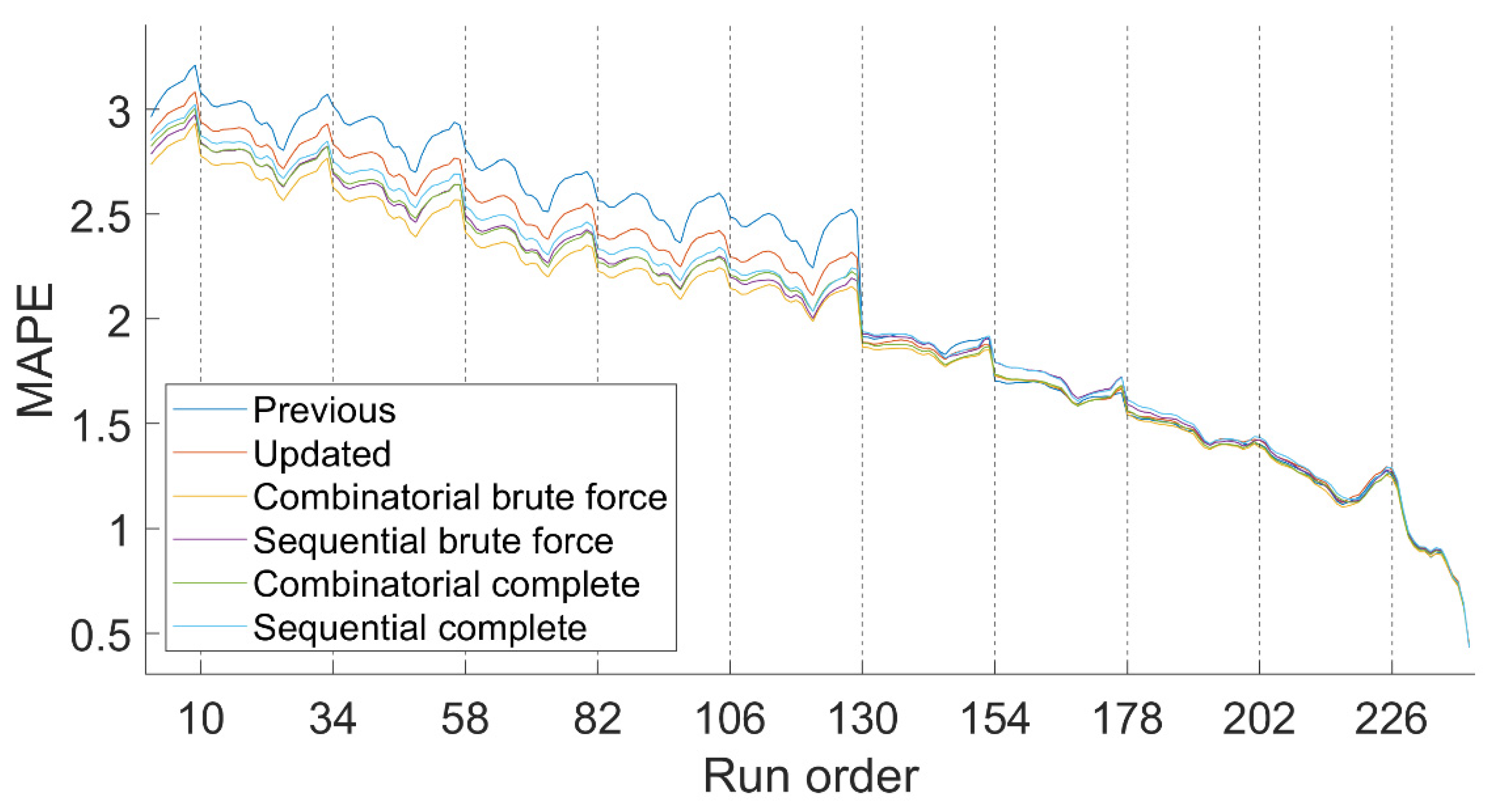
6.1. Autoregressive Model Accuracy

Figure 5 shows the MAPE for all of the hours of the year from every autoregressive system; in other words, from the autoregressive models with each preprocessing method, including the original standard system, which is named as Previous. Each MAPE value is displayed according to how long in advance the load has been predicted, from one hour to nine days before. The abscissa axis represents the order of execution in chronological order, so that the first execution is the one carried out at 12:00 a.m. on the previous ninth day. Temperature data arrive at 9:00 a.m. each day, and these moments are reflected in the graph with vertical dotted lines.

Table 1. Error Average of Autoregressive Models.

Name	MAPE (%)	RMSE (MWh)
Previous	2.149	863.33
Updated Forecasting System	2.069	831.48
Combinatorial Brute Force	1.964	789.86
Sequential Brute Force	2.010	802.82
Combinatorial Completeness	2.002	804.94
Sequential Completeness	2.039	815.67

shows the average error for each forecasting system from all forecast horizons, including RMSE.

All processing methods outperform Previous with 4 or more days in advance. During that interval, the Combinatorial Brute Force is consistently the best, considering MAPE and RMSE. The accuracy for the remaining days is very similar for all methods.

6.2. Autoregressive Error Difference vs. Time Ahead of the Forecast

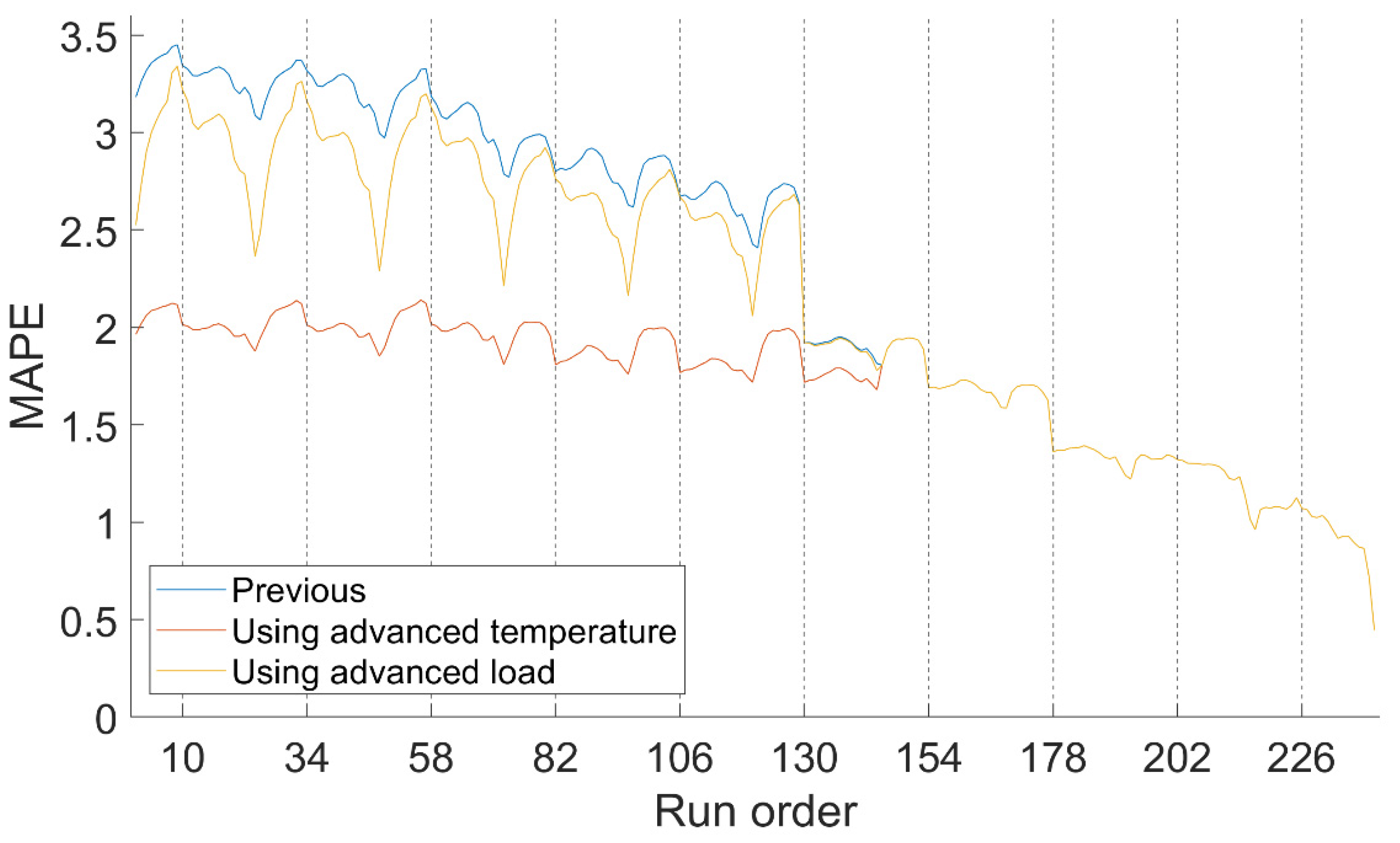
On the sixth day of execution, at 9:00 a.m. (execution 130) there is a very pronounced error jump on the previous version. At the time of the jump there are only two factors that vary: temperatures and last recorded load. To check which of these factors causes the jump, two versions of the old REE system have been trained: one acts as if temperature at the jump time was known in earlier forecasts; on the other hand, the second acts as if it was the load at jump time that was known. The respective simulation is shown in Figure 6.

Figure 6 allows us to conclude that it is temperature that lowers the accuracy during the first execution days, because the model using temperature from later days shows a very similar pattern until the seventh day.

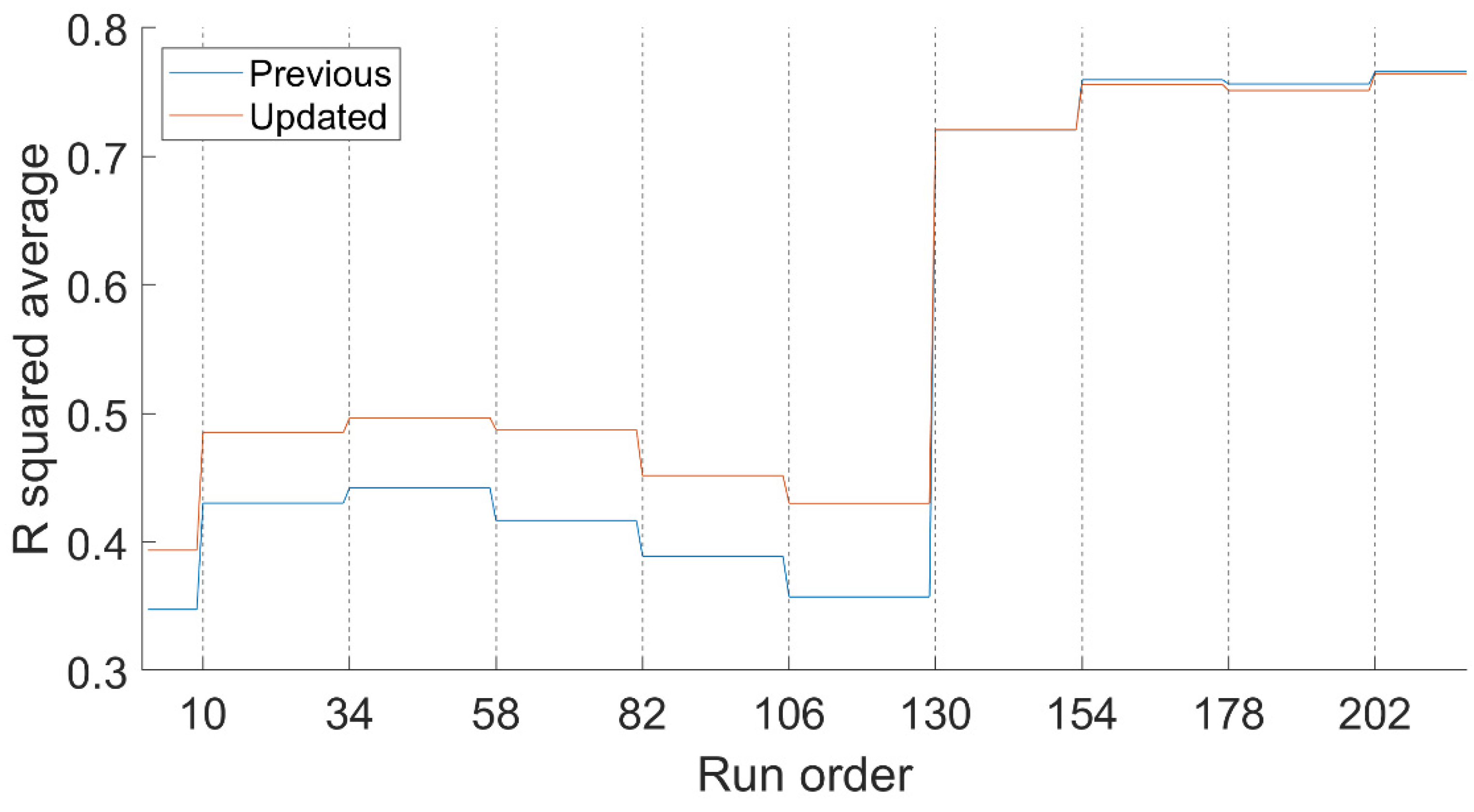
Once the temperature is located as a factor that causes this difference in precision, the correlation between temperature and demand was analyzed. For this, the time series of training temperature has been isolated; that is, variables CD, HD and their lagged versions. Subsequently, R squared values of these time series have been calculated. Finally, the R squared average for each anticipation has been drawn in Figure 7. The process is performed for the previous and updated system. Vertical lines indicate the moments when temperature data arrives. It has only been used on weekdays and working days to avoid the influence of other variables.

Correlation is constant between data collection moments, since during these intervals temperature time series do not change. Correlations behave similarly to precision. At 9:00 a.m. on the sixth day there is a jump. Previous to this jump, the updated system offers a better performance, while later there is no appreciable difference between systems. Therefore, a simple change to using hourly thresholds considerably improves the relationship between temperature and demand.

In conclusion, between available temperature variables and load, there is a correlation jump on the sixth day. This correlation variation causes the abrupt accuracy improvement, since accuracy depends on the accuracy of available temperature data.

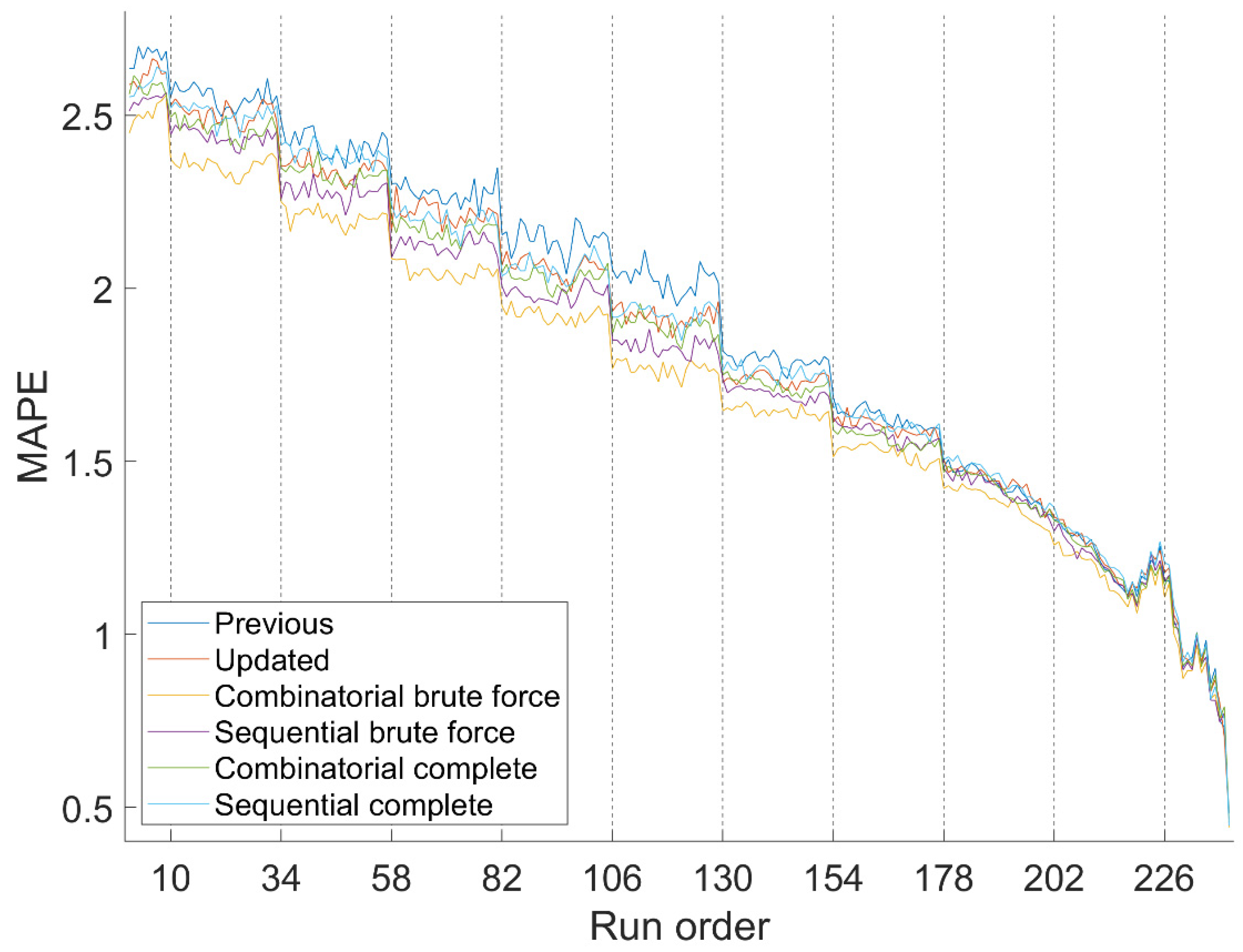
6.3. Hybrid Systems Accuracy

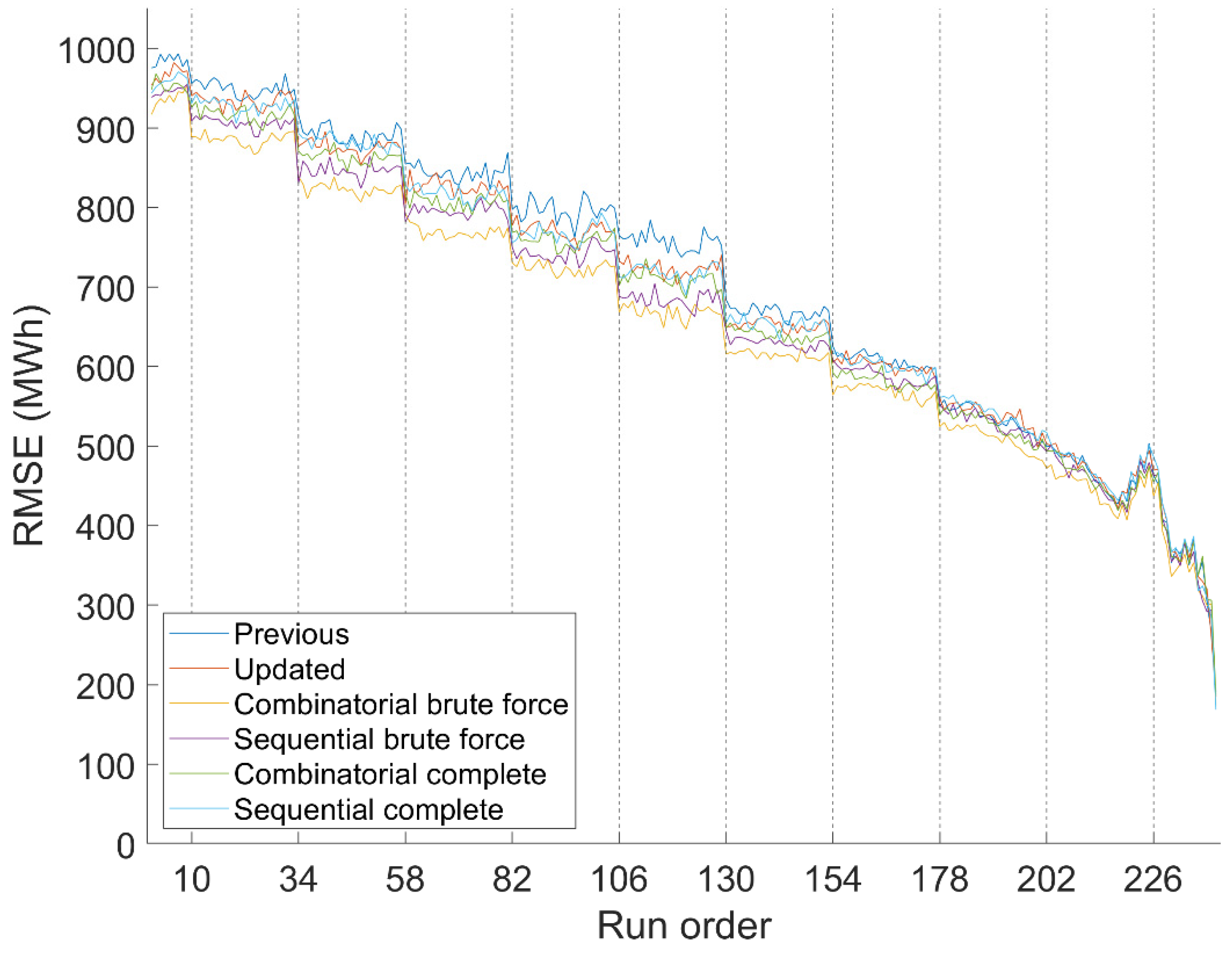
Figure 8 shows the MAPE of hybrid systems, since these produce the final forecasts for the operator, while Figure 9 shows the RMSE. To summarize data from Figure 8 and Figure 9,

Table 2. Error Average of Hybrid Systems.

Name	MAPE (%)	RMSE (MWh)
Previous	1.953	767.98
Updated Forecasting System	1.906	767.92
Combinatorial Brute Force	1.793	708.27
Sequential Brute Force	1.850	727.11
Combinatorial Completeness	1.878	737.28
Sequential Completeness	1.914	750.41

shows the error average of hybrid systems from all advances, also known as run orders.

Regarding both metrics, the Combinatorial Brute Force version is more accurate than the rest overall. It also offers better accuracy with almost all forecast horizons, so it consistently performs better. Combinatorial Brute Force is thus considered as the best preprocessing method for the REE forecasting system.

6.4. Autoregressive Interpretability

Once an autoregressive model has been obtained, it can be used to read its coefficients and draw conclusions from the training period.

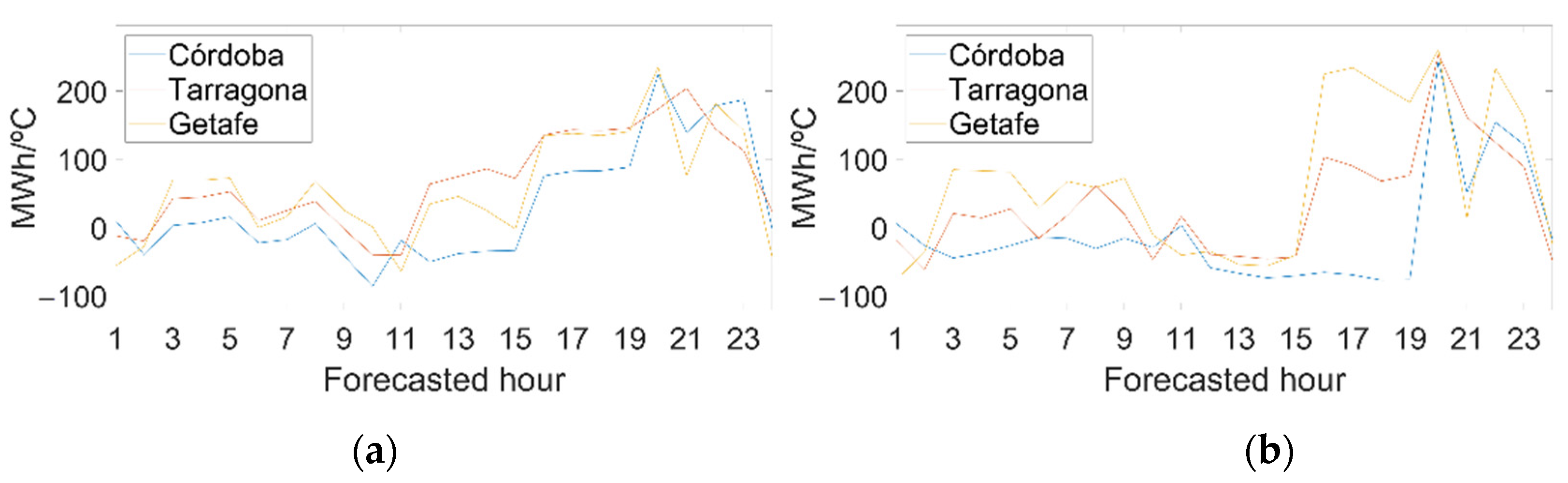
The winner procedure for the autoregressive model (Combinatorial Brute Force) has obtained three zones:Córdoba, Tarragona and Getafe. It has also obtained two previous days of temperature used at a peninsular level (nl), while at the local level it has obtained zero previous days in each of the zones (zl).

To quantify the change that one variable undergoes when another varies, sensitivity is calculated. Applying it to the autoregressive model of (3) through (15).

$$S_A=\frac{\partial y_t}{\partial A}=y_t^{\prime }{e}^{A{\Psi }_a}{\Psi }_a=y_t{\Psi }_a$$

(15)

where S_A is the sensitivity of any exogenous variable A. Since sensitivity depends on forecasted load, for each demand value there is a different sensitivity, instead of a fixed value, as would result from a linear model that predicts the demand directly, as shown in (16) and (17), which is not the case.

$$y_t={\displaystyle \sum }_{i=1}^d{c}_{t-i}{\beta }_i+{\displaystyle \sum }_{k=1}^n{X}_{kt}{\Psi }_k+{\epsilon }_t$$

(16)

$$S_A=\frac{\partial y_t}{\partial A}={\Psi }_a$$

(17)

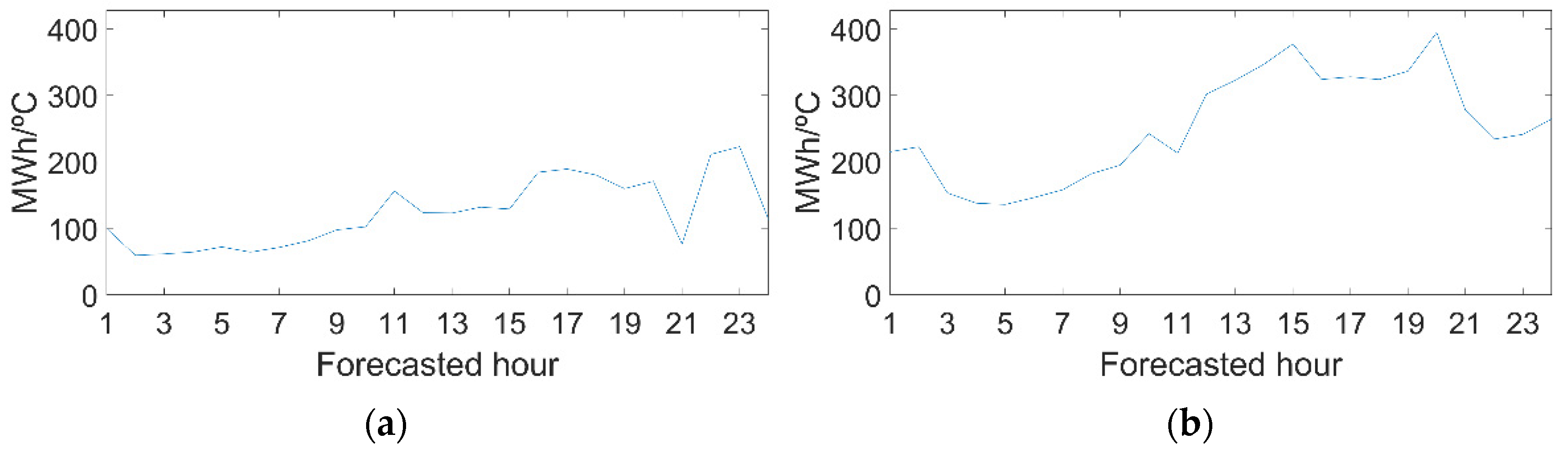
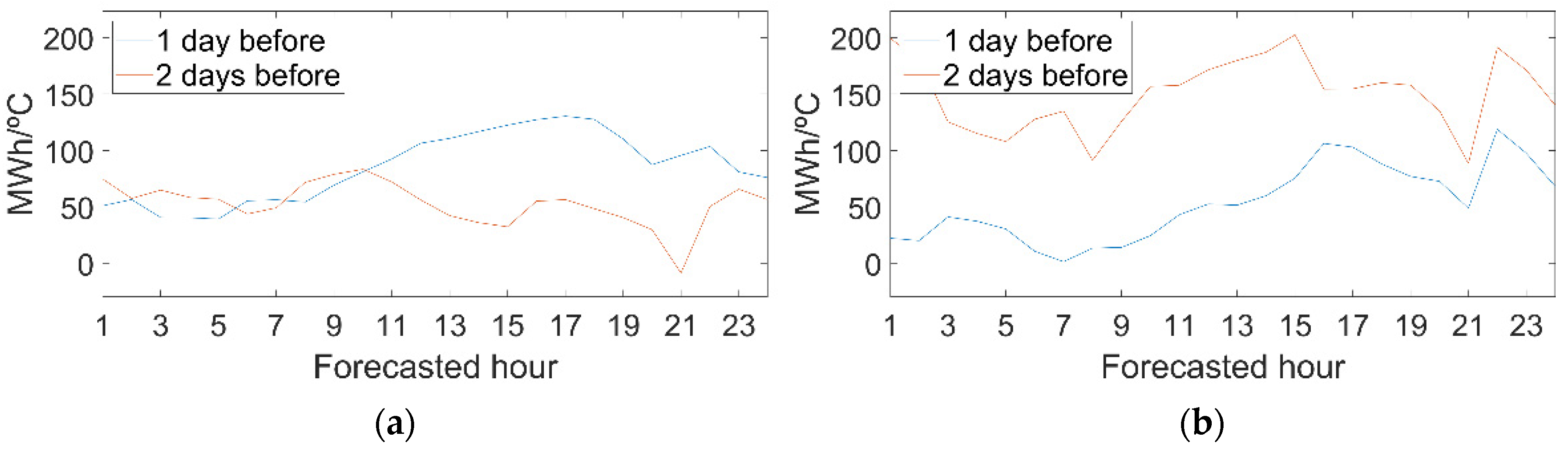
Once the autoregressive models have been trained with Sequential Brute Force, all hours of 2019 have been predicted, simulating the calculations that were made 9 days before at 5:00 p.m. The resulting demands have been multiplied by coefficients of their respective models, and then the sensitivities of 2019 have been obtained. Finally, sensitivity averages have been calculated, and they have been drawn on Figure 10, Figure 11 and Figure 12.

Since there are no previous individual days, sensitivities of their respective variables PIC_{z l} and PIH_{z l} do not exist. According to the algorithm used, individual previous days are not obtained because they do not improve forecasting accuracy. Therefore, they do not provide relevant information.

The sensitivities of peninsular heat are greater than cold (Figure 10); therefore, the heat effect is more influential than cold. In addition, both peninsular variables have lower values during the early morning hours, so temperature has less influence on rest periods.

On Figure 11 there are positive values. Therefore, on a peninsular scale, if it has been colder or hotter on previous days, the load will increase. In addition, in hot seasons the temperature of the second previous day has a greater influence than the previous one, while the opposite occurs for cold seasons.

Figure 12 represents the effect of one area being colder or hotter than the rest.

7. Conclusions

In this paper, a method has been developed to preprocess temperature data which improves the accuracy of forecasting electricity demand on a national scale. To do that, the peninsular demand of Spain for 2019 has been predicted. Preprocessing has been tested with the STLF system of the Spanish electrical operator REE. Forecasts have been made simulating the execution of the system with the same data availability that would be available under normal operating conditions. Simulations have been carried out for all horizons with the REE predictive system; therefore, its performance can be evaluated as the forecasted moment approaches.

Different data processing methods for temperature have been tested. The most accurate method selects five combinations of zones with the highest R squared with respect to the peninsular demand. Then, for each zone combination, all the combinations of the number of previous days of individual temperatures and their average are tested. Finally, we get the one that offers the best precision to predict the prior year to the one we wish to forecast.

The method of processing temperatures is automatic, so it selects the zones and variables with the greatest estimated influence on demand. Consequently, the implementation on a national scale does not require additional studies and the interpretability of the chosen zones is straightforward.

Incorporating temperature data preprocessing globally improves MAPE by 0.16% and RMSE by 59.71 MWh, as can be seen in Table 2. In addition, said improvement is consistent with respect to how early the forecasts are made, as shown in Figure 8 and Figure 9.

The new variables that are incorporated into the system are interpretable. The significance is expressed in Section Nomenclature, which allows for analysis with statistical models such as the REE autoregressive ones. These models also show an improvement in accuracy. The impact of the variables on the demand is obtained as the sensitivity expressed in (15). In addition, the sensitivity is expressed with an interpretable unit (MWh/°C). In the Spanish peninsula, the variable sensitivities show that hot temperatures influence load more than cold ones, but both have a lower influence on rest periods. According to the results, load is affected by the temperature of previous days, so heat from the second previous day has a notorious influence in the same way that cold from the previous day does.

It has been observed that the availability of temperature forecasts notably affects the accuracy of electricity demand, since there is a close relationship between how early a thermal forecast is made and the load forecasts. In conclusion, the most recent thermal forecasts for the forecasted moment should be used.

This paper is focused on predictive and non-analytic applications. In terms of future work, we propose to incorporate this new approach for processing temperatures into statistical models, and to use them as a tool to analyze relationships between temperature and electrical demand on both a national and regional scale, including smart grids. Another proposed future work is the implementation of the proposed methodology in other large-scale predictive system, in order to improve their accuracy and compare the employed preprocessing methods with different systems.

The sustainability of the energy systems is linked to the management of renewable resources, which, in turn, have a stochastic component that make them unreliable. The ability to forecast not only electric demand but also electric generation is key to ensuring an effective way to harness renewable energies. The preprocessing techniques described can also be applied to these fields where multiple climatological temperatures are used as input; for example, wind forecasting and, consequently, energy generation forecasting for wind generators and, therefore, can get us closer to a sustainable energy system.