Article

Estimating the Role of Climate Internal Variability and Sources of Uncertainties in Hydrological Climate-Impact Projections

1
College of Water Resources Science and Engineering, Taiyuan University of Technology, Taiyuan 030024, China
2
State Key Laboratory of Simulation and Regulation of Water Cycle in River Basin, China Institute of Water Resources and Hydropower Research, Beijing 100038, China
3
School of Water Resources, North China University of Water Resources and Electric Power, Zhengzhou 450045, China
*
Author to whom correspondence should be addressed.
Sustainability 2022, 14(19), 12201; https://doi.org/10.3390/su141912201
Submission received: 8 August 2022 / Revised: 15 September 2022 / Accepted: 15 September 2022 / Published: 26 September 2022

Abstract

:
Hydrological climate-impact projections in the future are limited by large uncertainties from various sources. Therefore, this study aimed to explore and estimate the sources of uncertainties involved in climate change-impacted assessment, in a representative watershed of Northeastern China. Moreover, recent studies have indicated that the climate internal variability (CIV) plays an important role in various hydrological climate-impact projections. Six downscaled global climate models (GCMs) under two emission scenarios, and a calibrated Soil and Water Assessment Tool (SWAT) model were used to obtain hydrological projections in future periods. The CIV and signal-to-noise ratio (SNR) are investigated to analyze the role of internal variability in hydrological projections. The results shows that the internal variability shows a considerable influence on hydrological projections, which need to be particularly partitioned and quantified. Moreover, it is worth noting the CIV can propagate from precipitation and ET to runoff projections through the hydrological simulation process. In order to partition the CIV and the sources of uncertainties, the uncertainty decomposed frameworks based on analysis of variance (ANOVA) are established. The results demonstrate that the CIV and GCMs are the dominant contributors of runoff in the rainy season. In contrast, the CIV and SWAT model parameter sets provided obvious uncertainty to the runoff in January to May, and October to December. The findings of this study advised that the uncertainty is complex in the hydrological simulation process; hence, it is meaningful and necessary to estimate the uncertainty in the climate simulation process. The uncertainty analysis results can effectively provide efforts for reducing uncertainty, and then give some positive suggestions to stakeholders for adaption countermeasures under climate change.

1. Introduction

Climate change is expected to impact on precipitation and temperature by the end of the 21st century; the changes in precipitation and temperature may substantially affect the regional and global hydrological cycle. Quantifying the response of runoff from climate change is directly associated with water resources management [1,2,3,4,5]. Global climate models (GCMs) are primary tools for providing future climate variables in a changing environment, which can be used to simulate the general circulation of the earth’s atmosphere, and which can provide credible information from past to future meteorological data [1]. Multi-model ensembles consisting of GCMs were used to drive the hydrological models (HMs) to obtain streamflow and other hydrological projections. It has become a useful method for estimating the hydrological process response to climate change in various regions of the world [6]. However, many uncertainties exist in the simulation process for future hydrological climate-impact projections. The different aspects of uncertainty in the model chain can be categorized as: (I) the internal variability of the hydrological climate-impact projections simulation; (II) scenarios uncertainty; and (III) model uncertainty [7,8,9,10,11,12,13].
Scenarios uncertainty is caused by the highly uncertain trajectory of the future socioeconomic development of human societies, and the lack of knowledge of future anthropogenic emissions of greenhouse gases (GHG) [14]. The scenario uncertainty is always shown, such as the different representative concentration pathway (RCP) emission scenarios for future periods.
Model uncertainty is due to a lack of ability to describe the real geophysical process, and is embodied in GCM and HM uncertainties. The GCM uncertainty mainly comes from the choice of the GCMs. Different GCMs are always simulated from different climate projections under the same emission scenarios. HM uncertainty is due to the model structure and model parameters. The mathematical formulas of the hydrological model can portray the rainfall and physical runoff process of the basin. Because of the lack of ability to describe the real world process, hydrological models are established using incomplete representations of reality [15], since this may result in model structure uncertainty. The contribution of parameter uncertainties significantly impacts on the model output; the different parameters may be due to the runoff changing in opposite directions [16]. In addition, parameter uncertainty is relatively easy to control via some conceptual or empirical parameters, and using an appropriate calibration method [17]. The inappropriate estimation of the main parameters may result in non-negligible uncertainty; for this reason, parameters uncertainty has received the most attention from previous studies [18].
Climate internal variability (CIV) is the natural variability of the climate system, and it includes the processes intrinsic to the atmosphere, the ocean, and the coupled ocean–atmosphere system, which are expected to present the natural viability of the regional climate on a multi-decadal time scale in the simulation chains [19,20]. Due to the chaotic variability of the climate system, the precipitation and temperature simulated using GCMs are influenced by the CIV [21]. The precipitation and temperature are important inputs of the hydrological simulation process; hence, the CIV in the climate system cascades to the hydrological processes [14]. Uncertainties due to the CIV are important uncertainty sources in hydrological projections [22]. Partitioning and quantifying CIV in a multi-replicate multi-model ensemble of hydro-meteorological projections, and estimating CIV under different emission scenarios are necessary for provide reliable forecasts and useful decision-making [23]. The internal variability of climate projections has been analyzed through many studies to estimate the uncertainty range of a chosen forced response, and to obtain a robust detection of climate change effects [24,25,26].
Generally, the attribute of hydrological climate-impact projections to CIV is a comparative concept of climate external variability effect via anthropogenic or natural changes in external forcing [27]. However, most of the studies focused on estimating the role of climate internal uncertainty in climate system projections, such as temperature and percipitation projections [28,29,30]. Upon consideration that internal variability may propagate in the hydrological simulation process and then affect the runoff uncertainty, quantifying the internal variabilities of precipitation, temperature, and ET can provide some useful information for runoff uncertainty analysis. Hence, the role of climate internal variability, GCM models, emission scenarios, hydrological model parameters and interaction effects in runoff projections is estimated and quantified in this study.
Clearly, partitioning CIV and external forcing are necessary for hydrological climate-impact projection uncertainties. Although some sources of uncertainty in hydrological climate-impact projections have been estimated in many studies, the CIV, scenarios, and model uncertainties need be equally investigated in the future literature. The role of the CIV in hydrological climate-impact projections is also rarely investigated.
To segregate the sources of uncertainties in hydrological climate-impact projections, Bosshard et al. [31] quantified the uncertainty contributions of an ensemble of hydrological climate impact projections by using the analysis of variance (ANOVA) method. In recently hydrological applications, the assessment framework based on ANOVA has been used to investigate the individual and interaction uncertainties from different sources [32,33,34,35,36]. However, the different kinds of uncertainty sources have not been estimated equally in previous research. They mainly aim for GCM decomposition, emission scenarios, the downscaling method, hydrological model structure, and parameters for the simulation process [34,35,37]. Moreover, investigating the role of internal variability in the overall climate change uncertainty can provide more useful information for the uncertainty estimation of the simulation process, and establish a more comprehensive framework of uncertainty analysis [24,25,26,38,39,40]. Therefore, comprehensive and systematic investigations for hydrological climate change impact, and an estimation of different sources of uncertainty is worthy and necessary.
The purpose of this manuscript is to estimate the contribution of sources of uncertainty, and to investigate the role of internal variability in hydrological climate-impact projections in a representative watershed of Northeastern China. This study has four purposes as follows: (1) to analyze the seasonal change in precipitation, temperature, ET, and runoff projections under climate change; (2) to partition and to quantify the source of uncertainty in hydrological climate-impact projections; (3) to investigate the role of internal variability in the hydrological climate-impact projections; and (4) to confirm the main impact sources of uncertainty in the hydrological simulation process. The findings of this research work may provide some meaningful suggestions regarding hydrological climate change impacts, and they present a methodology for partitioning uncertainty sources of runoff projections in a representative watershed in Northeast China.

2. Study Area and Data

2.1. Study Area

The Biliu River basin is located in Northeast China, spanning 39.54° to 40.35° N in latitude and 122.29° to 122.93° E in longitude, with an approximate area of 2085 km2 (Figure 1). The Biliu River Reservoir was built in 1975, and its storage capacity is 9.34 × 10⁸ m3. The mainly utility of this reservoir is water supply for nearby big cities and cropland irrigation. Another reservoir, called Yushi Reservoir, which was built in 2001 and is located upstream of Biliu River, with a storage capacity of 0.89 × 10⁸ m3 and a drainage area of 313 km2. Because the reservoir supplies water to the outside of the basin, the impact of Yushi Reservoir should thus be considered in the hydrological model. This study area has characterized the temperate monsoon marine climate, and the rainy season from June to September. The mean annual precipitation is 746 mm, the average annual temperature is 8.40 °C to 10.3 °C, and the maximum and minimum temperatures are 35.8 °C and −23.5 °C, respectively.

2.2. Data and Climate Change Scenarios

The historical observed daily meteorological datasets were available over the period of 1978–2004, and the monthly runoff datasets were available over the period of 1958–2011. These were obtained from the Biliu River Reservoir administration and Hydrology Bureau of Liaoning Province. The DEM (90 × 90 m), land-use map (1:100,000), and soil type map (1:1,000,000) are obtained from the Data Center for Resources and Environmental Science, Chinese Academy of Sciences.
The climate data were output from six GCMs in CMIP5 under the RCP4.5 and RCP8.5 emission scenarios: ACCESS1-0, BCC-CSM1.1(m), CESM1-BGC, CESM1-CAM5, CMCC-CM, and MPI-ESM-MR (Table 1). The climate data were extracted for the 1980–2004 period, 2041–2065 period, and 2066–2090 period, which were defined as a reference period, and two future periods, the 2050s and 2080s.

3. Methodology

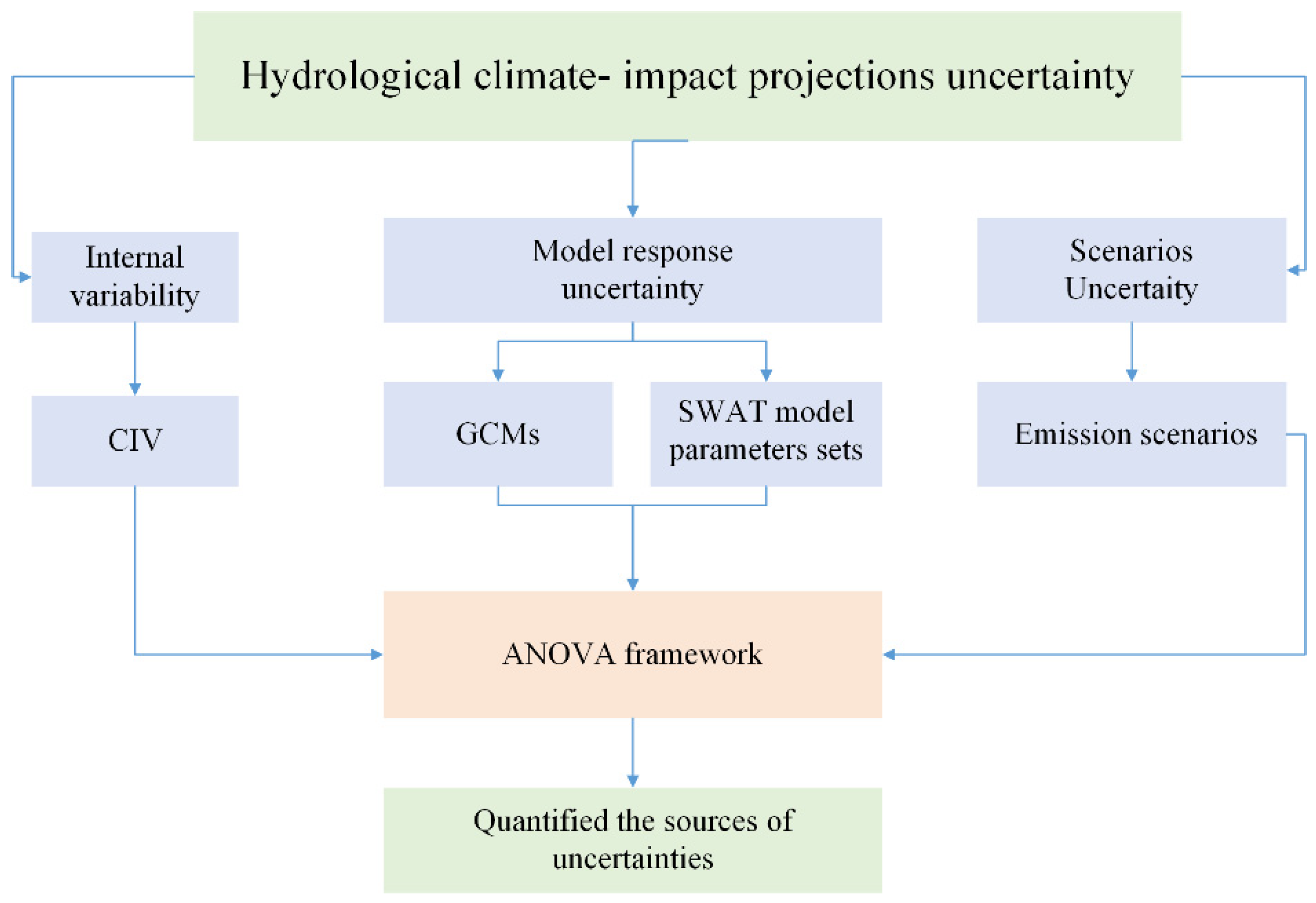
This manuscript combined six GCMs models under two representative concentration pathways (RCPs), which were based on the fifth phase of the Coupled Model Intercomparison Project (CMIP5). These climate change scenarios were downscaled using the morphing method, which uses an operation of shift or stretch to downscale the hydrological variability [41]. A widely used hydrological model, SWAT, was used for runoff simulation, and the SUFI-2 uncertainty approach for capturing the relatively uncertainty of the SWAT model parameters [42,43]. In order to obtain a robust detection of climate change effects, and to give some useful suggestions for practical decision making, the hydrological climate-impact projections in this manuscript contained precipitation, temperature, ET and runoff projections under climate change. The uncertainty decomposition framework of this study is shown in Figure 2.

3.1. Hydrological Modeling and Parameter Uncertainty Assessment

The SWAT 2012 was used to simulate runoff in this study. The SWAT is a physically based water-scale model that is widely used in investigating hydrological processes around the world [36]. The model divides the watershed into hydrologic response units (HRUs); each of these HRUs are based on a unique combination of soil, land use, and slope characteristics [44]. Recently, the model was developed to estimate the climate change impact on hydrological regimes under the prediction conditions over long periods of future. The SWAT-CUP software was utilized for calibration and the uncertainty assessment of parameters [42], the uncertainties in the output variables are exhibited in a 95% probability distribution (95PPU). The SUFI2 algorithm was chosen to calibrate and validate the parameters in the SWAT-CUP [43]. In order to account for the parameter uncertainty of the model, this manuscript used Latin hypercube sampling (LHS) to generate hydrological model parameter sets. The Nash–Sutcliffe efficiency (ENS), the average relative error (Re), and the coefficient of determination (R2) were used as the objective functions, measuring the distance between the observations and the simulations. Through sensitivity analysis of the calibration process, 11 hydrological parameters were generated. The initial iteration of LHS derived 1000 simulations for all initial parameter sets; the best 100 parameter sets were selected using the condition of ENS above 0.9, R2 above 0.9, and | R e | below 10.
The SWAT model was constructed based on the historical daily meteorological data and spatial geographic data of the study basin. The historical daily scale meteorological datasets were used to drive the SWAT model for both warm up, calibration and validation periods. Because the historical observed runoff datasets were all on a monthly scale, the model’s output monthly scale runoff data were compared with historical observed runoff data to evaluate the model performance. The SWAT model performance periods were divided into a warm up period (1978–1981), calibration period (1982–1996) and validation period (1997–2011). The simulated data from the SWAT were compared with the historical observed data to ensure their reliability.

3.2. Climate Change Scenario and Downscaling Method

CMIP5 has provided a future climate database and is widely available around the world [45]. Six GCMs from CMIP5 were selected to represent the future climate scenarios under the RCP4.5 and RCP8.5 emission scenarios. The SWAT model was driven by six GCMs and two emission scenarios, for a total of 12 ensemble scenario members under the 2050s and 2080s.
Because of the simple and easily used merits, this manuscript adopts the Morphing approach to remove biases from the original GCMs climate projections [45,46]. This method involves a shift, a linear stretch (scaling factor), and a combination of shift and a stretch [41]. The downscaled precipitation and temperature are calculated via Morphing, and show an acceptable performance in the study watersheds. More details of the downscaling process are shown in Zhu et al. [45].

3.3. Method of the CIV Estimation

In order to investigate the role of the CIV in hydrological climate-impact projections, the externally forced and internal variabilities need to be partitioned and quantified particularly. Generally, the internal variability is quantified using the “detrend” and “differenced” methods; the external forcing is subtracted from the hydrological variable series, and then the fluctuations of the variables are regarded as internal variability [47]. The average of a large number of ensemble members can average out the internal variability, and then the signal remaining is the response of the external forcing [48]. Hence, the internal variability can be obtained by subtracting the model-mean from each ensemble member [48]. The standard deviation of the ensemble variable or the residual to quantify the internal variability is the robust method, which has been applied in many previous publications [49,50].
C I V = 1 N i = 1 N ( 1 T 1 j = 1 T ( H c i , j H c i , j ¯ ) 2 )
where i and j are the ensemble number and the individual year; N and T are the total numbers of ensemble numbers and years, respectively; and Hc is the month time series of the hydrological climate-impact variables.
The key to estimating CIV is in partitioning the external forcing from the hydrological series, and the standard deviation of the given hydrological climate-impact projections is calculated as the internal variability [49]. The signal-to-noise ratio (SNR) is always used to quantify the relative contributions of internal variability and external forcing [21]. The SNR can provide useful information for investigating the magnitude of external forcing and the internal variability of hydrological climate-impact projections under future climate change. The model-mean of each ensemble is used as the signal, and the ensemble average of the sum of the squared difference between each member and ensemble mean is defined as noise [49]. The SNR is defined as the signal divided by noise.
n o s i e = 1 T ( N 1 ) j = 1 T i = 1 N ( H c i j H c j ¯ ) 2
H c j ¯ = 1 N i = 1 N H c i j

3.4. Source of Uncertainties Decomposition

3.4.1. The Hydrological Response to Climate Change

For any hydrological projections obtained from a hydrological simulation process for the ith member and jth time, the raw hydrological projections can be decomposed using the hydrological response to climate change and internal variability [49,50]. The raw hydrological projections Y i , j under climate change can be expressed as Equation (4).
Y i , j = φ i , j + η i , j
where φi,j is the hydrological response to climate change, and ηi,j is the deviation from the hydrological response obtained with the ith member and jth time, which can also be expressed as the internal variability.

3.4.2. Decomposition of the Hydrological Response to Climate Change

The hydrological response to climate change φi,j of any GCM/emission scenarios can be defined as Equation (5):
φ i , j = μ + α h + β k + γ l + ξ h , k , l
where μ is the overall mean of the hydrological response to climate change, αh is the effect contributed by the hydrological model parameters, βk is the effect contributed by GCMs, γl is the effect contributed by the emission scenarios, and ξh,k,l is the interaction terms of the model.

3.4.3. The Different Components of the Total Uncertainty

On the basis of the above expression of the raw hydrological response from the GCM/emission scenarios, the overall variance of the hydrological projections V a r [ Y h , k , l ] is as follows:
V a r [ Y h , k , l ] = V a r [ φ h , k , l ] + V a r [ η h , j , k ]
where V a r [ φ h , k , l ] is the total uncertainty in the hydrological response and V a r [ η h , j , k ] is the uncertainty of internal variability of the hydrological projections.
V a r [ φ h , j , k ] = V a r [ α h ] + V a r [ β j ] + V a r [ γ k ] + V a r [ ξ h , j , k ]
where V a r [ α h ] is the variance of the SWAT model parameters effects, V a r [ β j ] is the variance of the GCMs model effect, V a r [ γ κ ] is the variance of the emission scenarios, and V a r [ ξ h , j , k ] is the variance of the interaction effects.

3.4.4. Source of Quantifying Uncertainties

This manuscript constructs a three-way ANOVA framework to decompose the different uncertainty contributions; this technology has the ability to partition the total observed variance into different sources, and then quantify the contribution of the different sources to the total variance [51,52].
It is based on a biased variance estimator that underestimates the variance when the sample size is small. In order to diminish the bias effects caused by the different number of levels of the uncertainty factors, Bosshard et al. [31] proposed a subsampling method that was applied in this manuscript. This subsampling technology selected two samples from the large sample sets, and then a new sample could be generated for ANOVA. This manuscript selects two SWAT parameters sets out of the 100 sets; superscript j is replaced by g(h, i), which is a 2 × 4950 matrix, as in the following:
g = ( 1 2 1 3 1 100 2 3 2 4 98 99 98 100 99 100 )
Based on the ANOVA theory and the form of Equations (6) and (7), the ANOVA model can be expressed as Equation (9). It is composed of the mean effects of the SWAT model parameters (αh), the GCMs model (βk), the emission scenarios (γl), internal variability (ηh,j,l), and interaction effects (ξh,j,l). The mean effects can be computed as the deviation of each factors’ mean value, and the global mean M g ( , j ) , , .
M g ( h , j ) , k , l M g ( , j ) , , = α h + β j + γ l + η h , j , l + ξ h , j , l
In the ANOVA model, the total variance of the hydrological variable M g ( h , j ) , k , l is expressed as the total sum of squares (SST), and it can decompose into the individual variance of each effect:
S S T = S S A + S S B + S S C + S S I V + S S I
where SSA, SSB, and SSC are the uncertainty contribution of the SWAT model parameters, GCMs, and emission scenarios, respectively. SSIV is the internal variability, and SSI is the contribution of the interaction effects between the SWAT model parameters, GCMs, and emission scenarios.
Using this approach, the intercomparisons among the uncertainty contributions of the SWAT model parameter, GCMs, emission scenarios, internal variability, and the interaction effects are not affected by the different sampling numbers.

4. Results

4.1. Hydrological Model Parameters Calibrated and Uncertainty

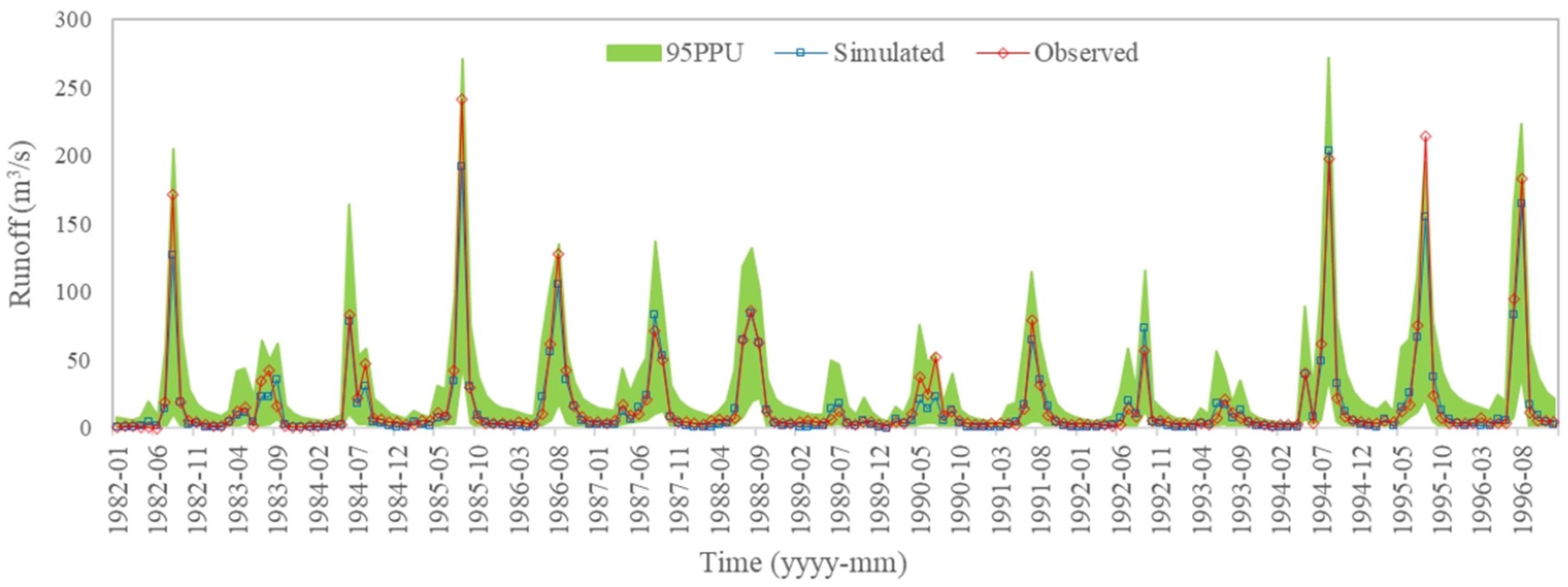
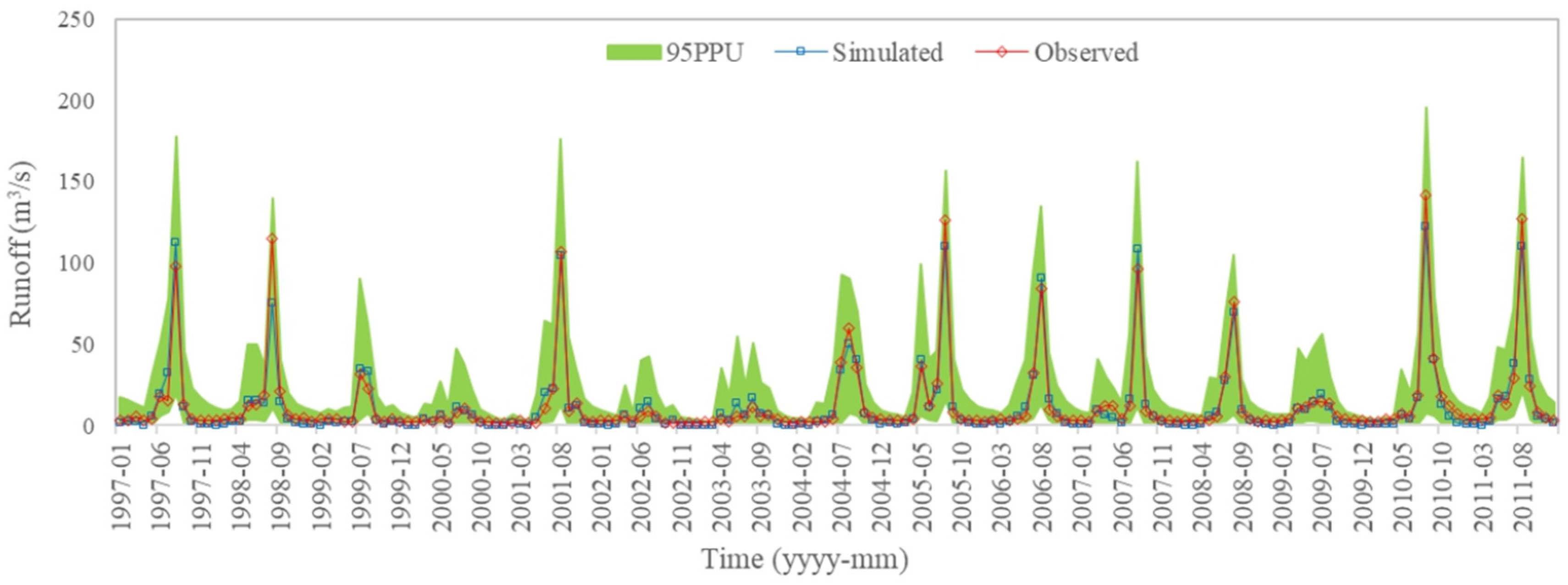
The SWAT model is constructed based on the historical daily meteorological data and spatial geographic data of the study basin. Before being used to predict the future runoff, the hydrological model parameters need to be calibrated and validated. The SUFI2 method is used to calibrate the parameters for the runoff in the study area for the 1982–2011 period. The parameters’ settings are shown in Table 2. The behavior parameter sets and the simulations are used to calculate the 95PPU as the uncertainty interval (Figure 3 and Figure 4). Moreover, the P-factor and R-factor were selected to estimate the performance of the uncertainty analysis method. Theoretically, a P-factor close to 1 and an R-factor is close to 0 indicate that the simulation exactly corresponds to the observed data [53]. In this study, the P-factor and R-factor are 0.97 and 0.81, respectively. This illustrates that more than 97% of the observed data are within the 95PPU band, and this demonstrates that the SWAT model was well applied in the study area.
The simulated data from the SWAT were compared with the historically observed data to ensure their reliability (Figure 3 and Figure 4). The metric ENS exceeds 0.94, while R2 exceeds 0.98. Re values are −0.91% in the calibration period, and ENS exceeds 0.95, while R2 exceeds 0.98. Re values are −5.38% in the validation period. More details about the calibration and validation were introduced in Zhu et al. [54].
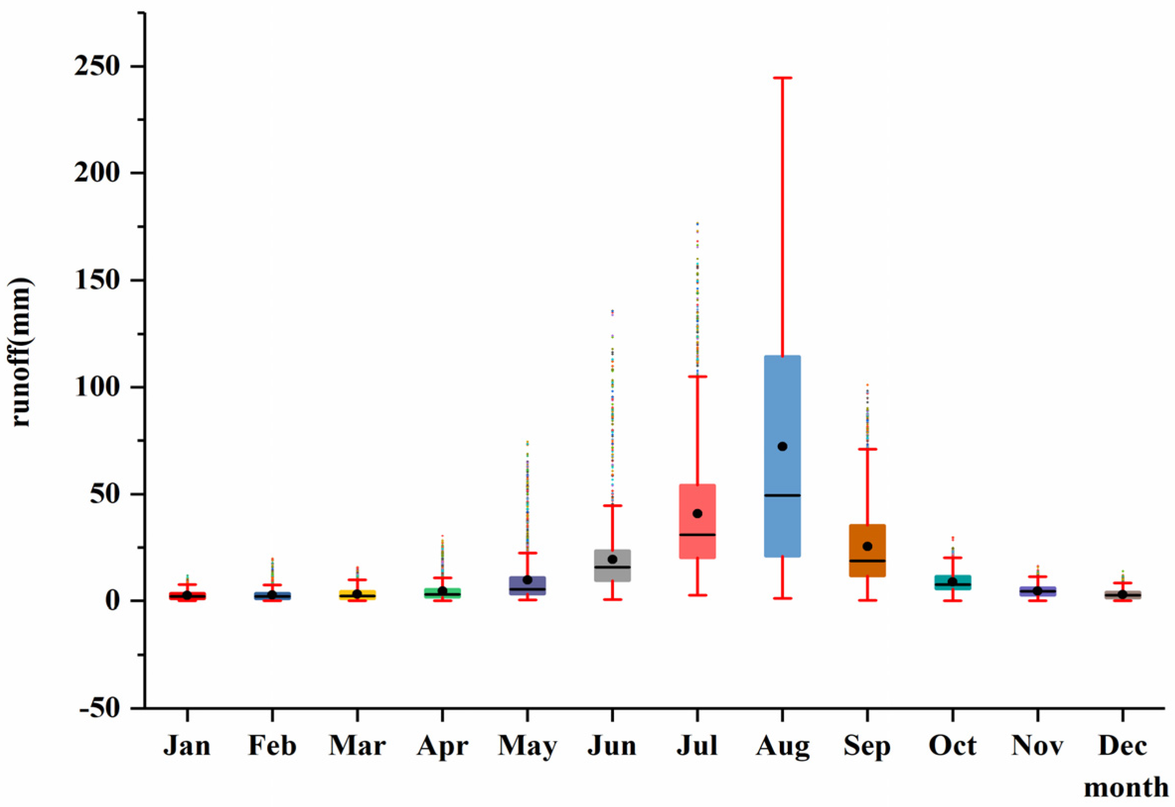
The SUFI2 algorithm is used as a parameter uncertainty estimate method for the reference period in the study basin. For a final ensemble of the 100 parameter sets generated by the LHS, these parameter sets are input into the SWAT model to generate 100 behavioral simulations, which are presented in Figure 5 with the help of box plots. Each box represents 100 behavioral simulations with outputs by the calibrated SWAT model. The length of the box plots denotes the runoff change range from 100 simulations, corresponding to one specific month. The differences between two boxes shows that the parameters effects are quite different for one given month. It can be seen in Figure 5 that the month runoff change range due to the SWAT model parameter sets are relatively larger in June to September. As June to September is the flooding season of the watershed, the uncertainty of runoff may play an important role in flood control and management. Hence, the uncertainty contribution of the SWAT model parameter sets needs be quantified.

4.2. Estimating the Uncertainties of Hydrological Climate-Impact Projections under Climate Change

4.2.1. Changes in Precipitation Projections

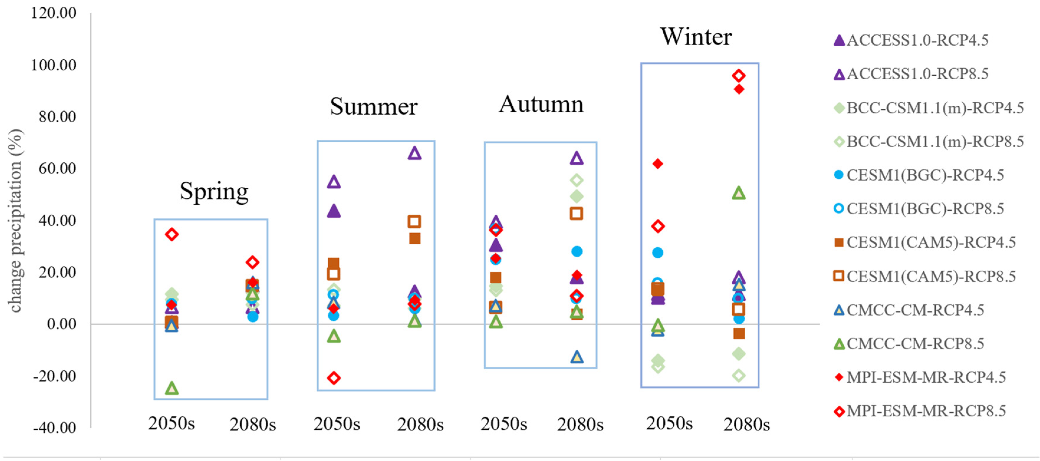
The precipitation projections for the 2050s and 2080s are compared with the reference period and are demonstrated in Figure 6. It can be seen that the performance of many scenario members showed a trend of marked increase in the 2050s and 2080s; however, several members showed a decreasing trend.
Taking the 2050s summer for example, all of the precipitation projections show an increased trend except for the performances of CMCC-CM and MPI-ESM-MR, which show a decreased trend under the RCP8.5 scenario; the precipitation changing interval ranges from a 54.13% increase to a −21.2% decrease. The uncertainty of the precipitation projections is significant in the 2080s winter, which changes from −19.79% to 95.95%. In contrast, the changing range of spring and autumn are relatively small. Among the two future periods, the uncertainty range of spring is from 31.2% to −21.27% in the 2050s, and the range of autumn is from 1.71% to 41.18% in the 2080s. Compared to the other seasons, the change range of spring is smallest in the 2080s.
The precipitation projections of different GCMs in the same emission scenarios and periods display a obvious changing range. It can be noted that the precipitation projections have non-negligible uncertainty in the future. This uncertainty of precipitation propagates through the hydrological model and is amplified in the runoff outputs. Hence, the precipitation uncertainty under climate change needs to be investigated beforehand.

4.2.2. Change in Temperature Projections

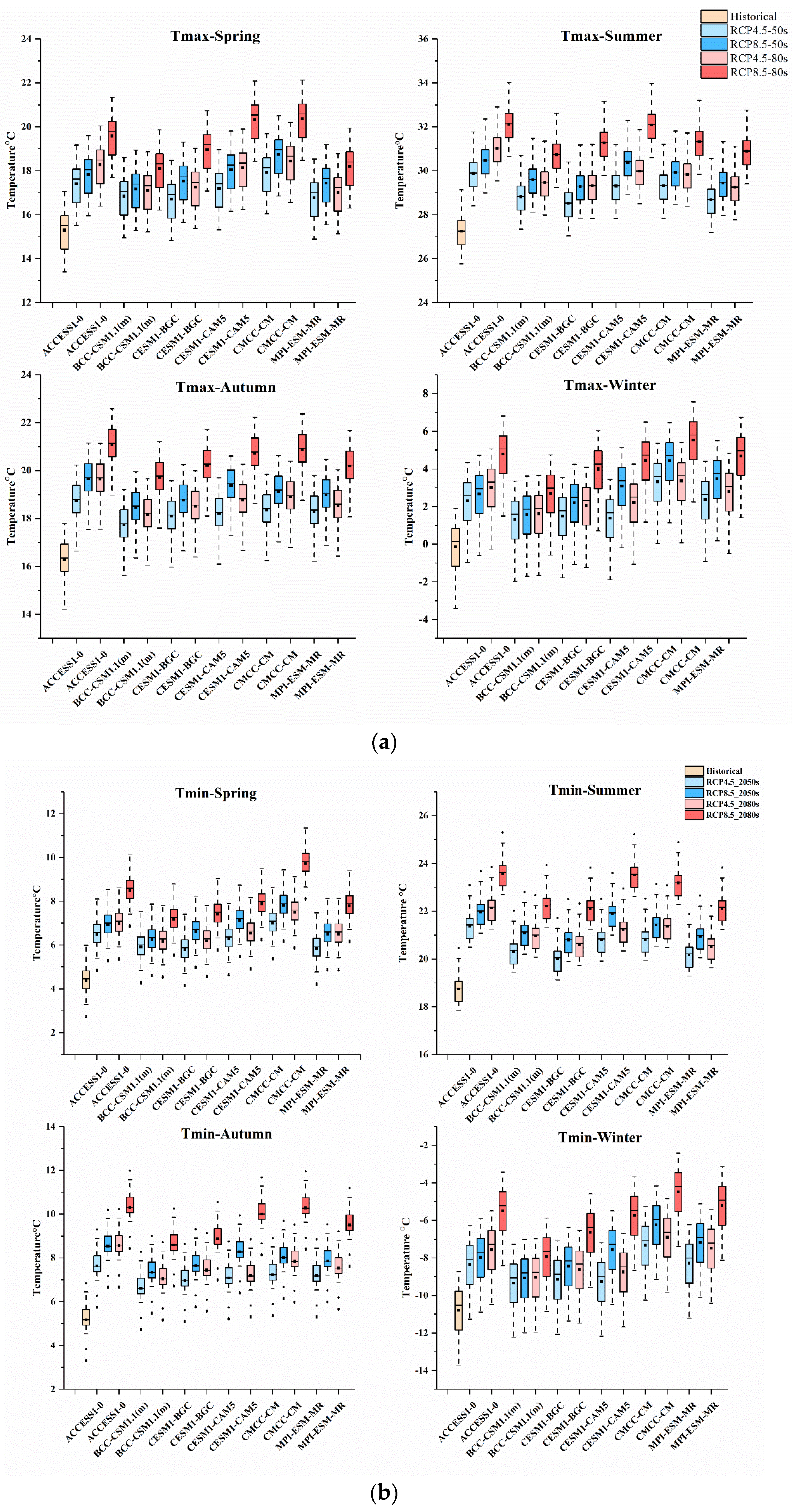
The box charts in Figure 7a,b show the maximum and minimum temperature projections (Tmax and Tmin) compared to the reference period. The temperature projections show a univocal increased trend for each scenario’s member. Specifically, in the 2050s period, the mean temperature increases are 1.95 °C under RCP4.5, and 2.73 °C under RCP8.5, while increases of 2.73 °C under RCP4.5, and 4.20 °C under RCP8.5 in the 2080s period are predicted. Moreover, the increase ranges of the Tmax are larger in summer and autumn than in the other seasons. The summer mean of Tmax increases by 1.84 °C and 2.52 °C in the two future periods under RCP4.5. Again, the increase range of Tmax is also significant under RCP8.5, where the increase in the mean Tmax is 2.61 °C in the 2050s summer and 4.17 °C in the 2080s autumn. The changing trend of Tmin shows a similar increasing trend in the two future periods, and the ranges of increase in the mean Tmin are all above 4.0 °C in summer, autumn, and winter under RCP8.5.
From the Tmax and Tmin changing results in the 2050s and 2080s under two emission scenarios, it can be found that the increase in temperature becomes larger as the time increases into the future period, and increased range is larger under RCP8.5 than RCP4.5. It can be also obtained that the uncertainty of temperature is marked in the future among different scenario members; the main uncertainty sources need to be quantified and estimated.

4.2.3. Change in ET Projections

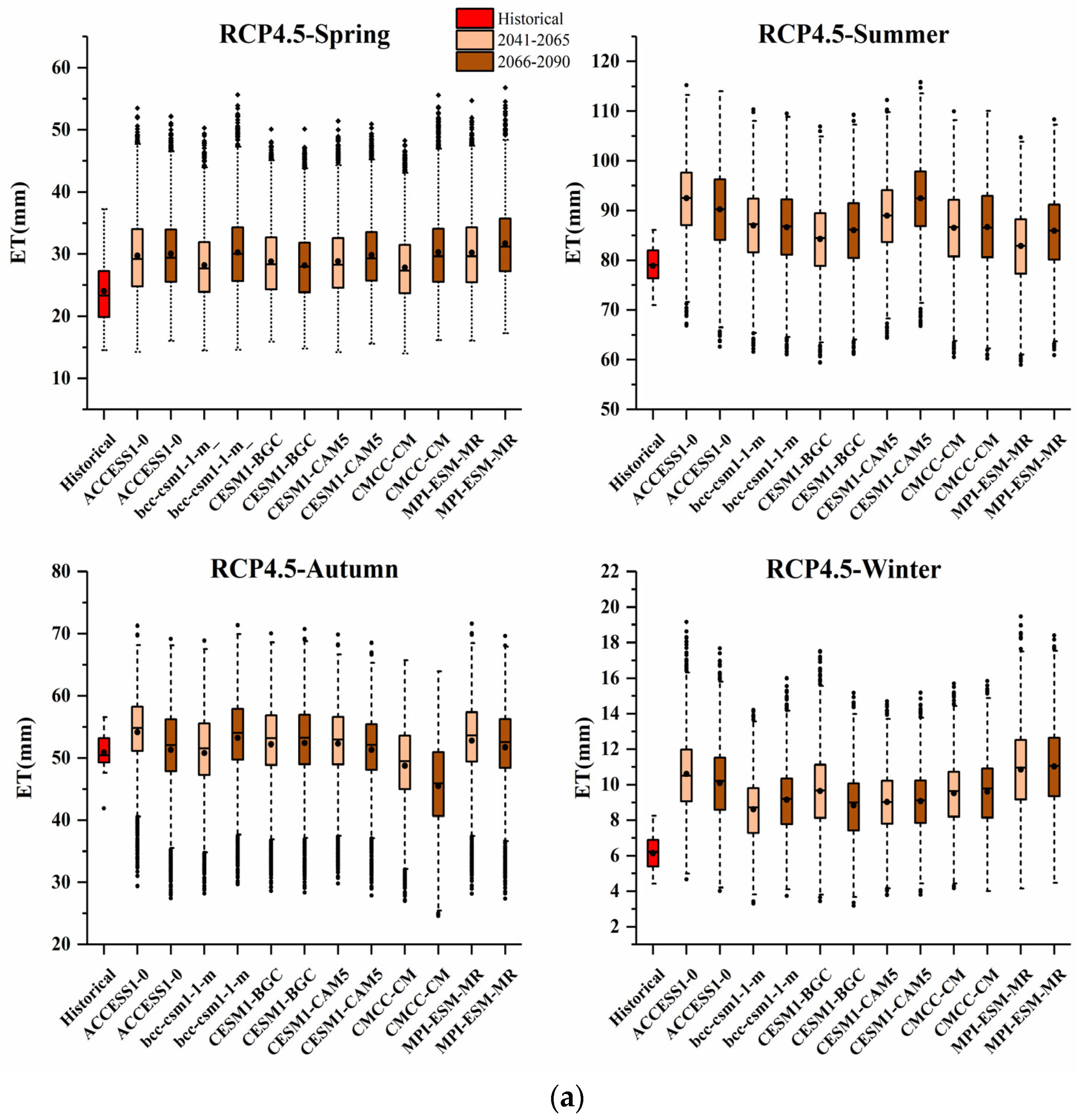
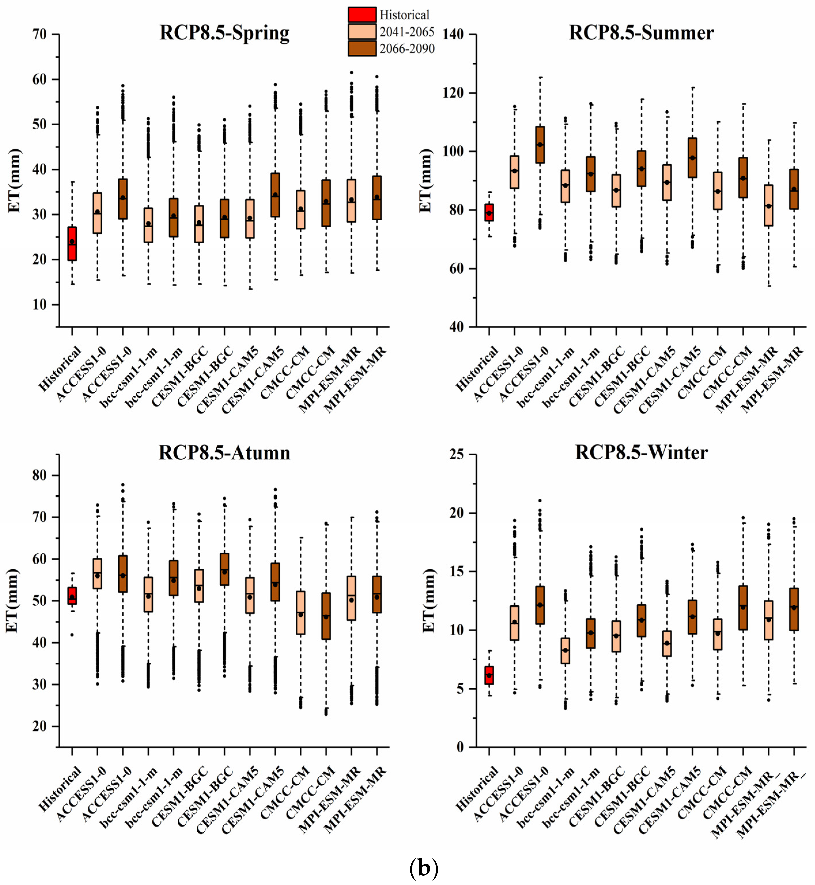
The calibrated hydrological model outputs 100 behavioral simulations for each scenario’s member in each month. There are 1200 sets of ET projections that can be obtained from the hydrological simulation for two future periods, and the future season of ET projections compared with the baseline period is shown in Figure 8a,b. For the RCP4.5 and RCP8.5 emission scenarios, the seasonal mean ET projections show an obvious increased trend in spring, summer, and winter. However, the mean ET of autumn demonstrates a relatively smaller increase, and some of the models show a decreased trend. In contrast with the precipitation and temperature projections, the various ET projections among each scenario’s members are relatively smaller.

4.2.4. Change in Runoff Projections

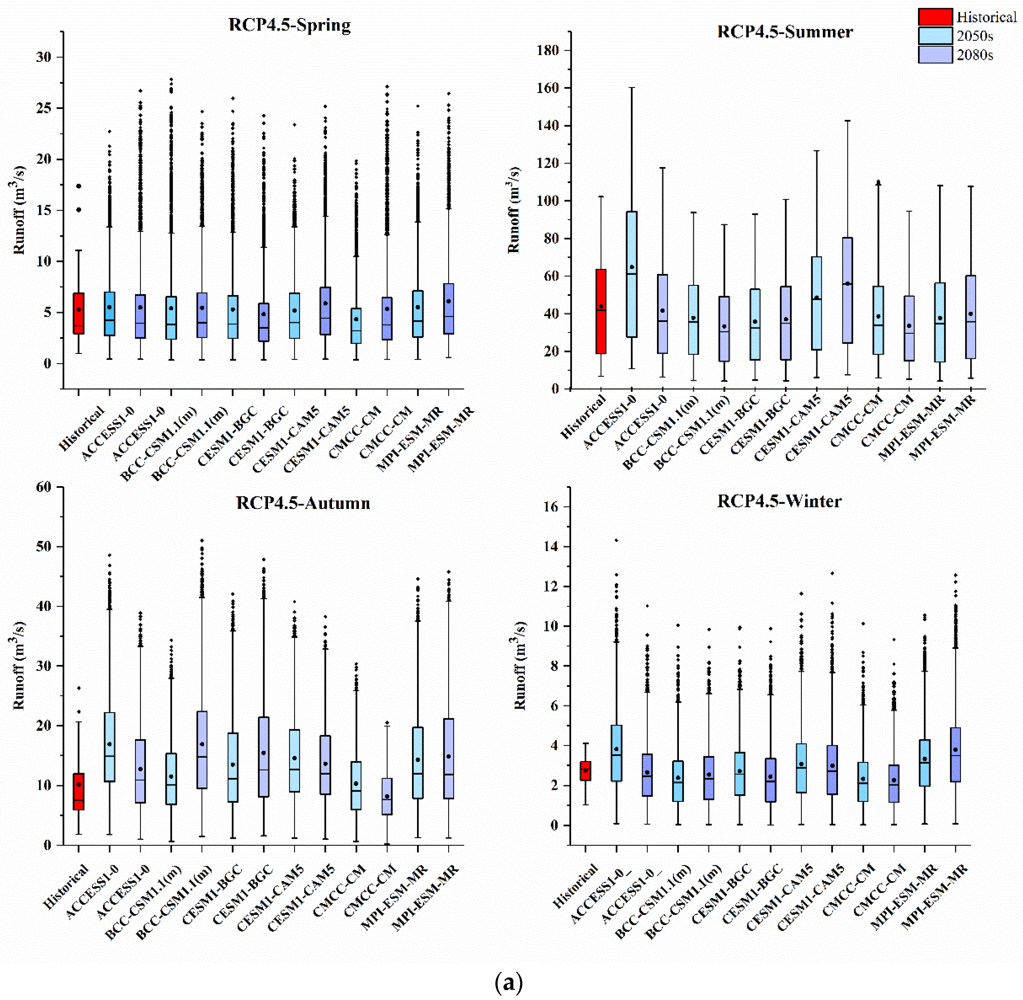
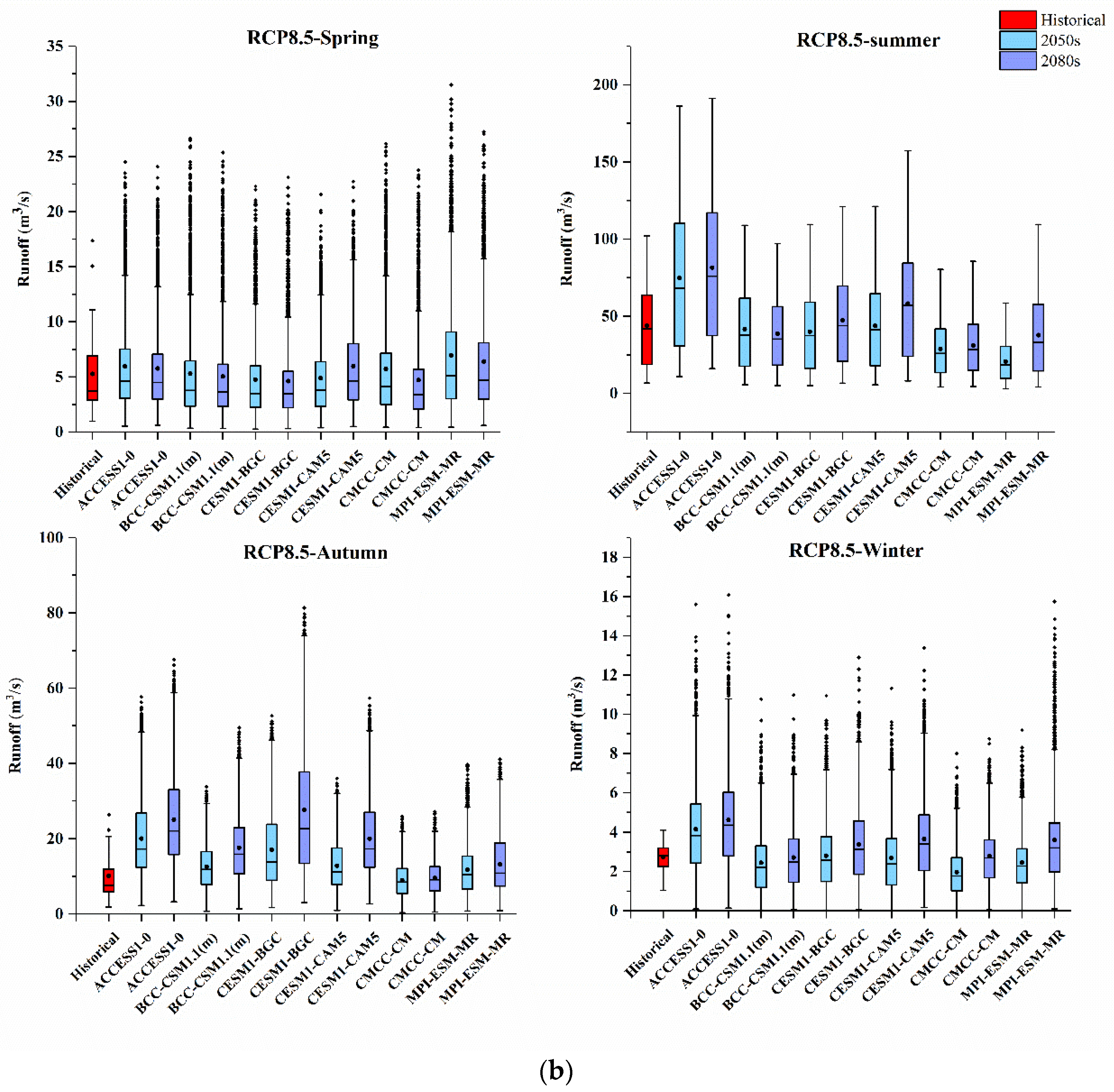
The predicted runoff projections of the four seasons in the two future periods are compared with the reference period in Figure 9a,b; each box and whisker plot for the runoff projections are generated from 1200 simulation chains. For the 2050s, the runoff projections increase more significantly in autumn than in the other seasons. In terms of the autumn runoff changing, many scenario members show an increased trend in the future, ranging over 1.37~66.01% under RCP4.5 and −11.99~97.08% under RCP8.5. In comparison with the autumn runoff, the runoff projections in summer trend a relatively small decrease in the future. The range of runoff change is −18.41% to 47.78% under RCP4.5 in the 2050s; there are four scenario members that demonstrate a decreased trend, such as BCC-CSM1.1(m) (−13.70), CESM1-BGC (−18.41), CMCC-CM (−11.81), and MPI-ESM-MR (−13.97). The range of runoff change is from −52.78% to 70.41% under RCP8.5 in the 2050s; it can be found that the diversity of the runoff is larger in this scenario, and that most of the scenario members shows a decreased trend in the future. For the 2080s, the obvious change in runoff is in summer and autumn. Most of the scenario members show an increased trend in autumn runoff; the mean changing ratio is 33.89% under RCP4.5. In contrast with the autumn runoff, the runoff change in summer shows a decreased trend, and the mean changing ratio is −8.56% under RCP4.5. Similarly, the runoff projections still display obvious differences among the scenario members. The changing trend of the runoff projections demonstrated a consistently increased trend under RCP8.5; the mean changing ratios of spring, summer, autumn, and winter are 2.91%, 11.95%, 85.22%, and 25.68%, respectively. Furthermore, the diversity of runoff projection is still significant in the 2080s under the RCP8.5 scenarios.
Furthermore, from the box-and-whisker plots shown in Figure 9a,b, the upper and lower ends represent the highest and lowest runoffs, and the change range indicates the uncertainty bound. Compared with the runoff in the reference period, the autumn runoff projections reveal a consistent increase in the mean and median values under both two emission scenarios and the future periods. Most of the summer runoff projections show a decreased trend in the future. From the runoff projections change results, each scenarios’ member demonstrated a wide uncertainty inner member range, and an obvious diversity among the different members. Accordingly, the uncertainty ranges of the runoff projections under the RCP8.5 projections are larger than the RCP4.5 scenarios. Compared with the other seasons, the summer runoff projections showed the largest uncertainty trends under the two emission scenarios in the future. Observing the median values, the summer and autumn projections in the 2050s and 2080s show non-negligible differences; for example, the median values for summer under the RCP4.5 scenario feature a decrease in projections as BCC-CSM1.1(m), CESM1-BGC, CMCC-CM, and MPI-ESM-MR, which range from −22.82% to −15.04%. In contrast, the median values show an increase from 45.55% to 13.79% in the projections of ACCESS1 and CESM1-CAM5. In addition, the median values for the spring runoff projections in the 2050s under RCP4.5 portray a consistent slight increase from 3.23% to 12.51%, and only the CMCC-CM projection shows a decrease as −12%. Overall, the runoff projected by all GCMs showed a large uncertainty in the two future periods. Comparing the 2050s and 2080s, it can be found that the lower ends become smaller and the upper ends become larger, which indicate that the uncertainty bounds increase from the 2050s to the 2080s. In addition, comparing the RCP4.5 and RCP8.5 scenarios, the uncertainty bounds of the RCP8.5 scenarios are always larger than RCP4.5.

4.2.5. Impacts of Climate Factors on Runoff Change

After analyzing the changes of the climate factors (precipitation, Tmax, Tmin, and ET) in the future, it can be found that the different climate factors perform different changing trends and uncertainties under climate change. The different climate factors may affect and produce different uncertainty contributions to runoff change; hence, it is important to analyze the relationship between climate factors and runoff projections. In order to determine the relationships between them, multiple linear regression was performed for each model chain using the changes of precipitation, Tmax, Tmin, and ET as the independent variables, and the runoff as the dependent variables [37].
The regression coefficients for runoff are shown in Table 3. In general, the increase in precipitation may cause a positive effect on runoff increase; this trend can be found in all of the models, scenarios, and coefficients at the 0.001 significance level. In contrast, the increase in the ET projections was negatively related to runoff, and there are seven projections at the 0.001 significance level. In addition, the increase in Tmax and Tmin may contribute to an increased trend of runoff; however, the coefficients did not pass the significance test, even at the 0.05 level. In most scenario members, the precipitation and ET had a significant influence on runoff projection, and temperature had a slight influence; hence, the internal variability of the climate factor needs to be investigated specifically.

4.3. Evaluation and Investigation of the Source of Uncertainty

4.3.1. Estimating the Role of Internal Variability

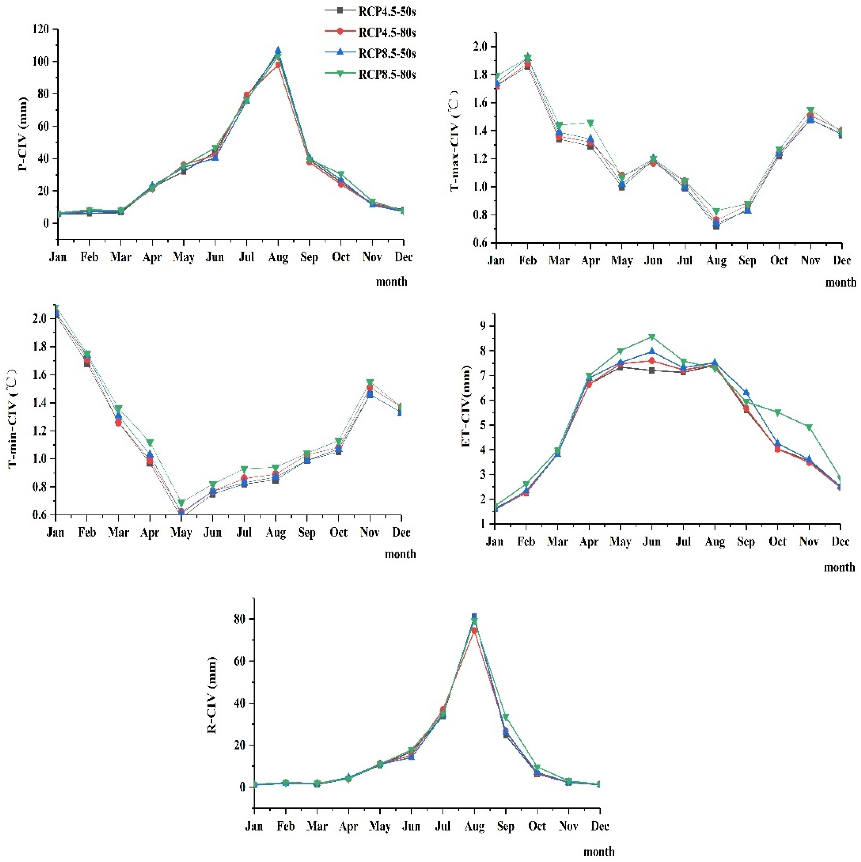
The role of internal variability in the hydrological climate-impact projections is partitioned and quantified in this section. In order to investigate the internal variability of the precipitation trends, six GCMs are forced by the same emission scenarios, and then the CIV values of the hydrological climate-impact projections under two emission scenarios are shown in Figure 10.
The CIV values of precipitation are higher in the rainy season (June to September), and the lowest values appear in winter. It is demonstrated that internal variability plays an important role on the uncertainty of flood season precipitation. Similarly, the CIV values of ET are larger in May to September than in the other months. In contrast, the CIV values of Tmax and Tmin are relatively smaller in the rainy season. Moreover, the CIV values of runoff demonstrate that the internal variability is higher in the rainy season than in the other seasons; this trend is similar to the CIV of the precipitation and ET projections. According to the multiple linear regression of the climate factors, precipitation and ET have significant influences on runoff, and this can imply that the internal variabilities of precipitation and ET may influence the internal variability of runoff.
From the CIV values of the runoff projections under the RCP4.5 and RCP8.5 emission scenarios, it can be found that the CIV values of the rainy season are larger than the other seasons, and that the maximum CIV value of the runoff projections appeared in August. Comparing the CIV values of precipitation, temperature, ET, and runoff projections, the internal variability of precipitation and runoff showed obvious increases in the rainy season. Upon consideration that the internal variability may combine with the model and scenario uncertainties and then influence the runoff, the contribution of internal variability needs to be specifically investigated.
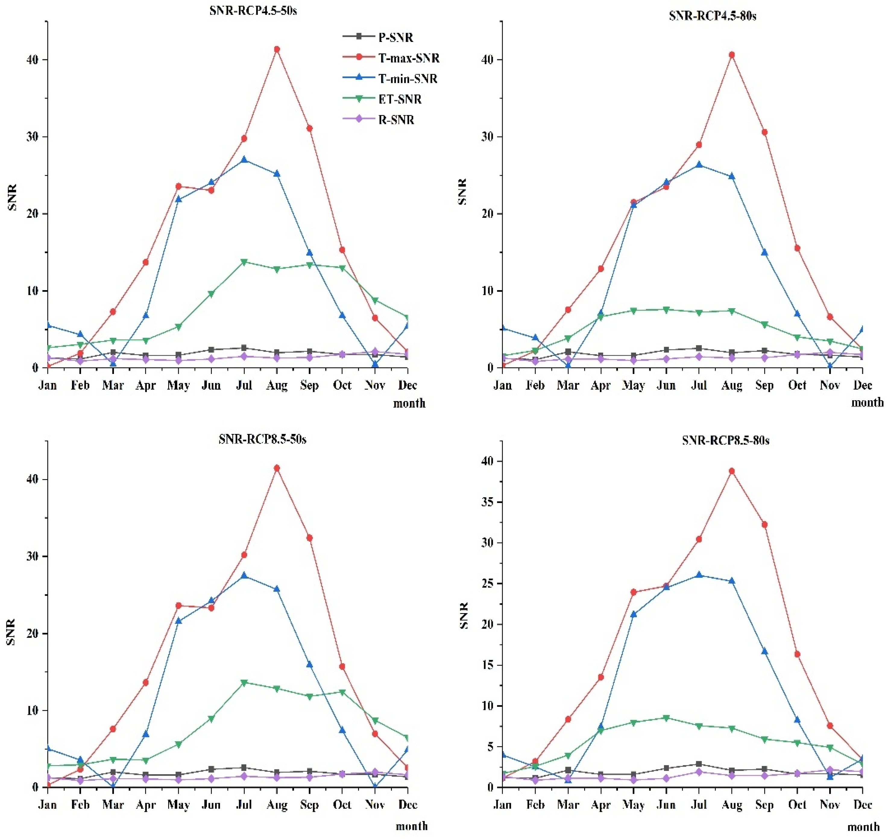
The SNR can give some useful information for investigating the role of internal variability. The SNR values of precipitation, temperature, ET, and runoff are shown in Figure 11. These metrics convey information about the magnitudes of the forced and internally generated components of hydrological climate-impact projections under future climate change. The SNRs of ET and temperature show an obvious change in spring, summer, and autumn. The SNR values of Tmax and Tmin demonstrated relatively higher values in June to October, and it was worth noting that external forcing is the main impact factor during these months. Similarly, the SNR of ET is higher in June to October than in the other months; hence, the internal variability of temperature and ET is weaker in this season. In contrast, the SNRs of precipitation and runoff are relatively stable among the four seasons. An important result is that the internal variability contributed a considerably higher component to precipitation and runoff than temperature and ET. On the basis of the estimation of internal variability, it can be observed that the SNR values of precipitation and runoff are mostly around 1 for each month. This means that the significance of internal variability is approximate with external forcing. However, the SNR values cannot quantify the internal variability. It is important to partition and to confirm the specific internal variability and other uncertainty source contributions that occur within a year.

4.3.2. Contribution Analysis of Uncertainty Sources

As mentioned previously, the uncertainty sources of hydrological climate-impact projections involve model uncertainty, scenarios uncertainty, and internal variability. The ANOVA method is used to quantify the uncertainty contribution of different sources of uncertainty in the 2050s and 2080s.
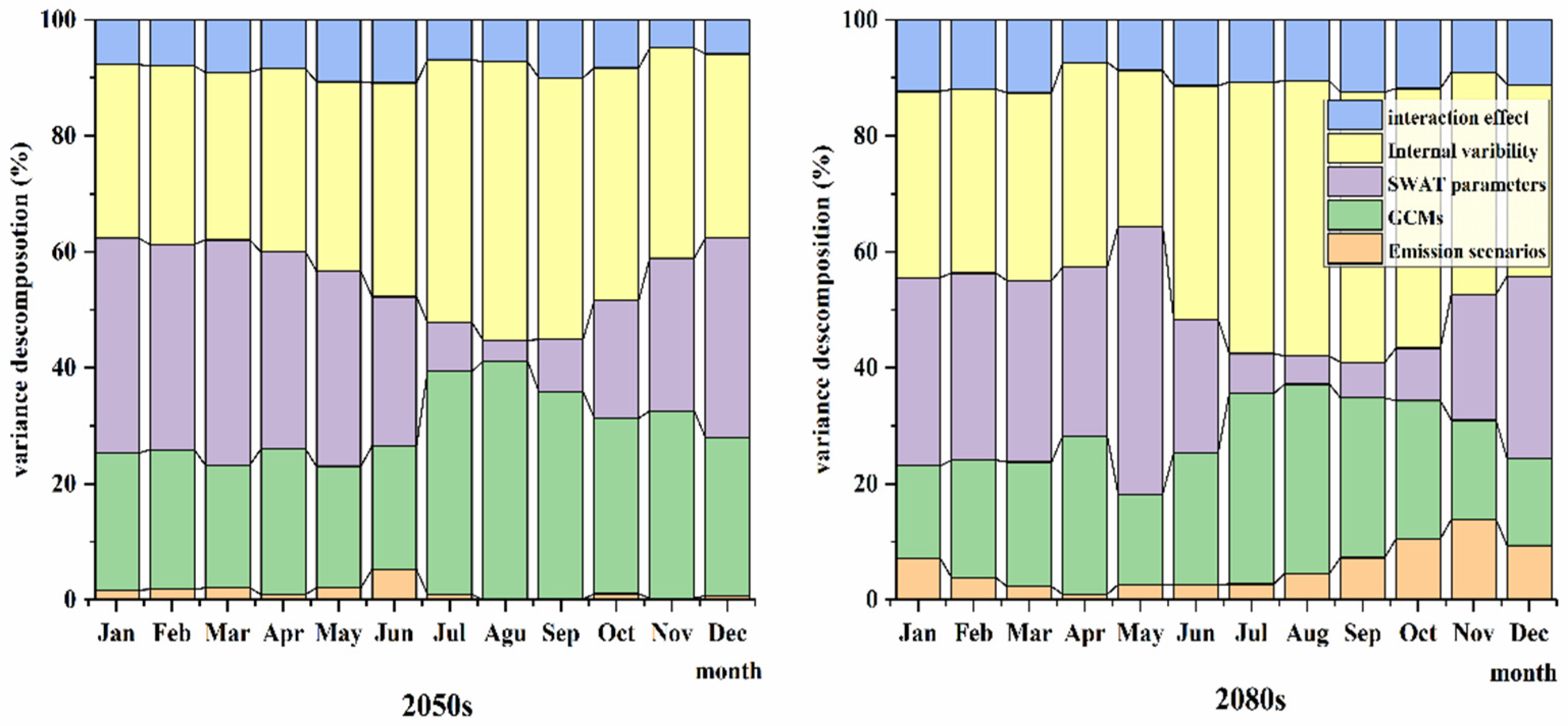
The contribution of uncertainty sources is shown in Figure 12. It is noteworthy that the effect of internal variability is significant for the entire month over the 2050s and 2080s period. The contribution of internal variability is almost equal to the sum of the uncertainty of GCMs and emission scenarios. It contributes 29~48% and 31.4~47.4% of the total variance in the 2050s and 2080s, respectively. Moreover, the biggest contribution is embodied in September in the two future periods. The other two main uncertainty contributors are the GCMs and SWAT model parameter sets. The uncertainty of GCMs account for 21~41% and 15~33% in the 2050s and 2080s, and the biggest value is in September (2050s) and August (2080s), respectively. For the SWAT model parameter sets, the contribution accounts for 4~39% and 4.8~32.4% in the 2050s and 2080s, respectively. Compared with the previous two uncertainty sources, the SWAT model parameters main affect the spring (March to May) and winter (December to February) runoff projections. The interaction term contribution to the runoff projection explains approximately 8~11% and 7~12% throughout the 2050s and 2080s periods, respectively. The contribution of the emission scenarios is relatively small, below 5% and 10.5% in the 2050s and 2080s, respectively.
Overall, the results of uncertainty decomposition in Figure 12 indicate that internal variability and GCMs are the dominant uncertainty contributors of runoff in June to October. In addition, the SWAT model parameters are the main uncertainty contributors in spring and winter. In summary, the internal variability and GCMs mainly provide the uncertainty contribution in summer and early autumn, and the main uncertainty contributors of runoff in spring and winter are the internal variability and SWAT model parameters.

5. Discussion

5.1. Hydrological Climate-Impact Projections Changes

This study estimated hydrological climate-impact projections changes under climate change impacts in a respective watershed in Northeastern China. Compared with the reference period, the temperature and precipitation projections demonstrated an increased trend in the two future periods, and this increased trend was more significant under the RCP8.5 emission scenarios and the later future period (2080s). This finding is consistent with some previous publications. Wang et al. [36] found that the response of hydrological extreme events to climate changing was much higher in 2070–2099 under the RCP8.5 scenarios. In addition, the ET projections showed an obvious increase trend in summer and winter, and a relatively small increase trend in autumn. It can be found that the runoff projections show an increased trend in autumn and a slightly decreased trend in summer. With the combined influence of increasing the precipitation, temperature, and ET in summer, there is a high possibility that runoff would decrease in summer. In contrast, a relatively slight increase in ET in autumn may be due to the runoff increase. Since precipitation, temperature, and ET are important inputs to the hydrological model, the uncertainties of these projections may thus also influence the runoff projections. Moreover, through multiple linear regression analysis, the precipitation and Tmax had a significant positive effect on runoff, and ET and Tmin show a relatively small negative effect on runoff. Hence, the increase in precipitation and the relatively small increase in ET may be due to a relatively obvious increase in autumn.
This manuscript also found that the prediction of both hydrological climate-impact projections showed a wider range under RCP8.5 than RCP4.5, especially in the 2080s. Moreover, the projected runoff in the future also demonstrated an obvious diversity in the future, especially in summer and autumn. To deal with the uncertainty in future runoff, the details of sources of uncertainties need to be investigated and quantified, so that relatively reliable hydrological projections are produced.

5.2. The Role of Internal Variability

Since the internal variability plays an important role in the uncertainties of the hydrological climate-impact projections, the CIV of future projections has thus been investigated under RCP4.5 and RCP8.5. The findings have indicated that the internal variability of precipitation, ET, and runoff are larger in June and September than in the other months. In order to investigate the magnitudes of external forcing and internal variability, the SNRs of future projections have been investigated under RCP4.5 and RCP8.5. The SNR values of precipitation and runoff are stable; the values are all around 1 among the 12 months, which means that the internal variability and external forcing performances have an equality effect. However, using the SNR values alone, it is difficult to determine what is the important influential factor for the hydrological climate-impact projections. Considering that June to September contains the entire flood season in the research watershed, the annual internal variability and external forcing uncertainty contribution of the runoff projections need to be particularly investigated.

5.3. Estimating the Source of Uncertainties

The ANOVA framework was constructed to quantify that the uncertainty sources contribute to the overall uncertainty; furthermore, in considering the substantial effects of internal variability on the uncertainty of the runoff projections, the uncertainty contribution of internal variability has been considered to ensure the comprehensiveness of the uncertainty assessment.
Quantifying the source of the uncertainties contribution to future runoff projections can provide insights into finding the main effecting factors of runoff variety under climate change. On the basis of the SNR values of different projections, the internal variability and external forcing of precipitation and runoff show equal significance, which can be embodied in uncertainty estimations. In the rainy season (June to September), the internal variability and GCMs are the mainly uncertainty contributors in the runoff projections. In contrast, the internal variability and SWAT model parameter sets provide obvious uncertainties to the runoff in January to May, and October to December.
These findings indicate that climate internal variability is the most important uncertainty source among the different sources chosen by this study, agreeing with the findings of some previous publications [50]; however, most of these studies focused on estimating the role of climate internal uncertainty in climate system projections, such as temperature and percipitation projections [28,29,30]. Meanwhile, the runoff projections are significantly impacted by the choices of GCMs; this point has also been found in many studies [34]. For instance, Zhang, et al. [55] found that the disparity between different GCMs may mainly impact on climate change research, and that the increased sample size of GCMs may conduct a complete uncertainty assessment. As an important tool for runoff simulation and prediction, the hydrological model is a non-negligible uncertainty contributor of overall uncertainty; among the uncertainty derived from the hydrological model, the model parameters obtained more attention [26,35] Moreover, the contribution and interaction effects are relatively small compared with the other uncertainty sources; these findings are consistent with some previous studies [31,33].
The quantification of climate internal viability has been demonstrated in several previous studies [49,50]; however, most of the studies focused on estimating the role of climate internal uncertainty in climate system projections, such as temperature and percipitation projections [28,29,30]. Upon consideration that internal variability may propagate in the hydrological simulation process and then affect the runoff uncertainty, quantifying the internal variabilities of precipitation, temperature, and ET can provide some useful information for runoff uncertainty analysis. Hence, the role of climate internal variability, GCM models, emission scenarios, hydrological model parameters and interaction effects in runoff projections is estimated and quantified in this study. For the rainy season, the internal variability and GCMs are the dominant uncertainties for runoff. On the basis of multiple linear regression, precipitation and ET have a significant influence on runoff, and their uncertainties can also influence runoff uncertainty. From the CIV and SNR values of the climate projections, it can be found that the internal variabilities of precipitation and ET are large in the rainy season. Hence, the internal variabilities of precipitation and ET may affect runoff to some extent. Above all, the internal variability plays an obvious role in shaping the overall uncertainty, and some of the uncertainty sources of the runoff projections can be traced back to precipitation and ET, etc.

5.4. Uncertainty and Limitation

There are lots of uncertainties inherent in the analysis of hydrological impacts, and the primarily contribution may come from hydrological model structures, hydrological model parameters, input data, GCMs, and downscaling methods.
Note that the hydrological model structure as well as model parameters sets represent the major sources of uncertainty in hydrological simulation. Aryal et al. [52] used two hydrological models to estimate the model uncertainties. In this study, the performance of the SWAT model is good in hydrological simulation, and the P-factor and R-factor are 0.97 and 0.81 in the calibration period, respectively. Moreover, the model parameters’ uncertainty was considered in the uncertainty analysis framework. The results indicate that the parameters play an important role in uncertainty analysis. However, the input land use and land cover data during the calibration and validation period can only express the land use and land cover pattern for a certain year. In order to avoid underestimation of the land use and land cover variance, different land-use conditions need be used to drive the hydrological model [36]. The remotely sensed data can provide precise demonstrate for land use and land cover, which can be used to analyze the hydrological variables changing [56]. Hence, more accurate land use and land cover data need be used in hydrological uncertainty estimation in future study.
It needs be noted that the downscaled future climate scenarios will also attribute a considerable uncertainty [57]. Generally, multi-model ensemble climate models are always using to reducing the uncertainty [26,34,37]. In this study, 6 GCMs were used to generate 12 climate scenarios; however, more GCMs need be chosen when evaluating hydrological responses to climate change.

6. Conclusions

The details of sources of uncertainty in hydrological climate-impact projections have been investigated and quantified in this manuscript. The uncertainties in quantification and estimation are essential for the runoff prediction. In addition, identifying fundamental uncertainty sources is meaningful for reducing existing uncertainties in the future. The main conclusions of this study can be summarized as the following:
(1)
Based on this study, which is an analysis of the future climate conditions for the Biliu River basin, it can be found that precipitation and temperature show an increasing trend in the future, especially in RCP8.5 and in the later future period. In addition, the climate factors may produce different influences and uncertainty contributions to runoff change. For instance, the precipitation has a significant positive effect on runoff, and ET shows a relatively small negative effect. Hence, the change in precipitation and ET may be due to a corresponding change in runoff. Furthermore, wide uncertainty ranges can be found in each projection, and sources of uncertainty may have obviously influenced the reliability of the future hydrological process simulation.
(2)
By elucidating the impact of climate internal variability on runoff projections, this study analyzes the role of internal variability of hydrological climate-impact projections and determines the important influencing factors of uncertainty for runoff projections. In terms of precipitation and ET, the internal variability is larger in June to September, and the SNR values also show that internal variability and external forcing are both important influencing factors for runoff. Combining with the internal variability and GCMs are the dominant uncertainty contributors in June to September. It is worth noting that the internal variability can propagate in the hydrological simulation process, and that the internal variability of runoff projections is remarkable in the flood season of the study watershed in the future. For the rainy season in the study basin, some water resources adaptation measures need be planned to alleviate the influence of climate change, especially in high emission scenarios (RCP8.5) and in the far future (2080s).
(3)
The uncertainty contribution of internal variability with the GCMs and SWAT model parameters is temporal variability. The internal variability and GCMs are the main uncertainty contributors for runoff projections in the rainy season (June to September). In contrast, the internal variability and SWAT model parameter sets provided obvious uncertainty to the runoff in January to May, and October to December. There are many studies focused on estimating the role of climate internal uncertainty in climate system projections, such as temperature and precipitation projections. This study investigated the role of climate internal variability, GCM models, emission scenarios, hydrological model parameters and interaction effects in runoff projections. The findings of this study indicate that the role of internal variability for hydrological climate-impact projections is noticeable in the future; these kinds of effects may greatly influence stakeholders and local water resource governments to provide appropriate hydrological regulations and flood control measures.

Author Contributions

Conceptualization, W.C. and J.L.; methodology, X.Z. (Xueping Zhu); software, X.Z. (Xuehua Zhao); validation, W.C., J.L. and X.Z. (Xuehua Zhao); formal analysis, X.Z. (Xiaoli Zhang); investigation, W.C.; resources, J.L.; data curation, W.C.; writing—original draft preparation, W.C.; writing—review and editing, W.C.; visualization, J.L.; supervision, J.L.; project administration, X.Z. (Xueping Zhu); funding acquisition, W.C. and X.Z. (Xiaoli Zhang). All authors have read and agreed to the published version of the manuscript.

Funding

This study was sponsored by the Natural Science Foundation of Shanxi Province, China. Grant No.202103021223113 and the Open Research Fund of State Key Laboratory of Simulation and Regulation of Water Cycle in River Basin, China Institute of Water Resources and Hydropower Research, Grant NO. IWHR-SKL-202103. Key Scientific and Technological Project of Henan Province (Grant No. 182102311062).

Institutional Review Board Statement

Not applicable.

Informed Consent Statement

Not applicable.

Data Availability Statement

The climate data in 1901–2099 for RCP4.5 and RCP8.5 were downloaded from the National Climate Center (http://ncc.cma.gov.cn accessed on 31 August 2022). The long-term experiment data of 1850–2100 for the chosen six climate models in CMIP5 were downloaded from the Program for Climate Model Diagnosis and Itercomparison (PCMDI, http://pcmdi3.llnl.gov/esgcet/ accessed on 31 August 2022). Yearly and monthly precipitation and runoff data in 1958–2011 were obtained from the Biliu River Reservoir administration. Month meteorological data were obtained from the China Meteorological Data Sharing Service System (http://cdc.cma.gov.cn/inex.jsp accessed on 31 August 2022). The Digital Elevation Model (DEM) data (90 × 90 m) were obtained from the CGIAR Consortium for Spatial Information (CGIAR-CSI) (http://srtm.csi.cgiar.org accessed on 31 August 2022). Soil type and land use maps were obtained from the Data Center for Resources and Environmental Sciences, Chinese Academy of Sciences (http://www.resdc.cn/fist.asp accessed on 31 August 2022). The calculate code of climate internal variability and ANOVA are according to the corresponding formulas, which has already described in this manuscript.

Acknowledgments

We would also like to acknowledge the World Climate Research Programme’s Working Group on Coupled Modeling, which is responsible for CMIP.

Conflicts of Interest

The authors declare that they have no known competing financial interests or personal relationships that could have appeared to influence the work reported in this paper.

References

  1. Zhang, Y.; You, Q.; Chen, C.; Ge, J. Impacts of climate change on streamflows under RCP scenarios: A case study in Xin River Basin, China. Atmos. Res. 2016, 178–179, 521–534. [Google Scholar] [CrossRef]
  2. Wang, B.; Liu, D.L.; Waters, C.; Yu, Q. Quantifying sources of uncertainty in projected wheat yield changes under climate change in eastern Australia. Clim. Change 2018, 151, 259273. [Google Scholar] [CrossRef]
  3. Vaghefi, S.A.; Iravani, M.; Sauchyn, D.; Andreichuk, Y.; Goss, G.; Faramarzi, M. Regionalization and parameterization of a hydrologic model significantly affect the cascade of uncertainty in climate-impact projections. Clim. Dyn. 2019, 53, 2861–2886. [Google Scholar] [CrossRef]
  4. Anjum, M.N.; Ding, Y.; Shangguan, D. Simulation of the projected climate change impacts on the river flow regimes under CMIP5 RCP scenarios in the westerlies dominated belt, northern Pakistan. Atmos. Res. 2019, 227, 233–248. [Google Scholar] [CrossRef]
  5. Yuan, S.; Quiring, S.M.; Kalcic, M.M.; Apostel, A.M.; Evenson, G.R.; Kujawa, H.A. Optimizing climate model selection for hydrological modeling: A case study in the Maumee River basin using the SWAT. J. Hydrol. 2020, 588, 125064. [Google Scholar] [CrossRef]
  6. Champagne, O.; Arain, M.A.; Leduc, M.; Coulibaly, P.; McKenzie, S. Future shift in winter sreamflow modulated by the internal var-iability of climate in southern Ontario. Hydrol. Earth Syst. Sci. 2020, 24, 3077–3096. [Google Scholar] [CrossRef]
  7. Byun, K.; Chiu, C.-M.; Hamlet, A.F. Effects of 21st century climate change on seasonal flow regimes and hydrologic extremes over the Midwest and Great Lakes region of the US. Sci. Total Environ. 2018, 650, 1261–1277. [Google Scholar] [CrossRef]
  8. Li, L.; Diallo, I.; Xu, C.-Y.; Stordal, F. Hydrological projections under climate change in the near future by RegCM4 in Southern Africa using a large-scale hydrological model. J. Hydrol. 2015, 528, 1–16. [Google Scholar] [CrossRef]
  9. Chen, J.; ST-Denis, B.G.; Brissette, F.P.; Lucas-Picher, P. Using Natural Variability as a Baseline to Evaluate the Performance of Bias Correction Methods in Hydrological Climate Change Impact Studies. Am. Meteorol. Soc. 2016, 17, 2155–2173. [Google Scholar] [CrossRef]
  10. Ficklin, D.L.; Letsinger, S.L.; Stewart, I.T.; Maurer, E.P. Assessing differences in snowmelt-dependent hydrologic projections using CMIP3 and CMIP5 climate forcing data for the western United States. Hydrol. Res. 2016, 47, 483–500. [Google Scholar] [CrossRef]
  11. Lee, M.H.; Bae, D.H. Uncertainty Assessment of Climate Change Impacts on Hydrology: A Case Study for the Central Highlands of Vietnam. Procedia Eng. 2016, 154, 617–623. [Google Scholar] [CrossRef]
  12. Nóbrega, M.T.; Collischonn, W.; Tucci, C.E.M.; Paz, A.R. Uncertainty in climate change impacts on water resources in the Rio Grande Basin, Brazil. Hydrol. Earth Syst. Sci. 2011, 15, 585–595. [Google Scholar] [CrossRef]
  13. Shen, M.; Chen, J.; Zhuan, M.; Chen, H.; Xu, C.-Y.; Xiong, L. Estimating uncertainty and its temporal variation related to global climate models in quantifying climate change impacts on hydrology. J. Hydrol. 2018, 556, 10–24. [Google Scholar] [CrossRef]
  14. Lafaysse, M.; Hingray, B.; Mezghani, A.; Gailhard, J.; Terray, L. Internal variability and model uncertainty components in future hydrometeorological projections: The Alpine Durance basin. Water Resour. Res. 2014, 50, 3317–3341. [Google Scholar] [CrossRef]
  15. Gupta, A.; Govindaraju, R. Propagation of structural uncertainty in watershed hydrologic models. J. Hydrol. 2019, 575, 66–81. [Google Scholar] [CrossRef]
  16. Zhang, R.; Corte-Real, J.; Moreira, M.; Kilsby, C.; Birkinshaw, S.; Burton, A.; Fowler, H.J.; Forsythe, N.; Nunes, J.P.; Sampaio, E.; et al. Downscaling climate change of water availability, sediment yield and extreme events_ application to a Mediterranean climate basin. Int. J. Climatol. 2019, 39, 2947–2963. [Google Scholar] [CrossRef]
  17. Wu, H.; Chen, B. Evaluating uncertainty estimates in distributed hydrological modeling for the Wenjing River watershed in China by GLUE, SUFI-2, and ParaSol methods. Ecol. Eng. 2015, 76, 110–121. [Google Scholar] [CrossRef]
  18. Nerantzaki, S.D.; Efstathiou, D.; Giannakis, G.V.; Kritsotakis, M.; Grillakis, M.G.; Koutroulis, A.G.; Tsanis, I.K.; Nikolaidis, N.P. Climate change impact on the hydrological budget of a large Mediterranean island. Hydrol. Sci. J. 2019, 64, 1190–1203. [Google Scholar] [CrossRef]
  19. Deser, C.; Phillips, A.; Bourdette, V.; Teng, H.M. Uncertainty in climate change projections: The role of internal variability. Clim. Dyn. 2012, 38, 527–546. [Google Scholar] [CrossRef]
  20. Pesce, M.; Critto, A.; Torresan, S.; Giubilato, E.; Pizzol, L.; Marcomini, A. Assessing uncertainty of hydrological and ecological parameters originating from the application of an ensemble of ten global-regional climate model projections in a coastal ecosystem of the lagoon of Venice, Italy. Ecol. Eng. 2019, 133, 121–136. [Google Scholar] [CrossRef]
  21. Deser, C.; Phillips, A.; Alexander, M.A.; Smoliak, B.V. Projecting north American climate over next 50 years: Uncertainty duo to internal variability. J. Clim. 2014, 27, 2271–2296. [Google Scholar] [CrossRef]
  22. Hawkins, E.; Sutton, R. The Potential to Narrow Uncertainty in Regional Climate Predictions. Bull. Am. Meteorol. Soc. 2009, 90, 1095–1108. [Google Scholar] [CrossRef]
  23. Van Doi, M.; Kim, J. Projections on climate internal variability and climatological mean at fine scales over South Korea. Stoch. Hydrol. Hydraul. 2020, 34, 1037–1058. [Google Scholar] [CrossRef]
  24. Steinschneider, S.; Wi, S.; Brown, C. The integrated effects of climate and hydrologic uncertainty on future flood risk assessments. Hydrol. Process. 2015, 29, 2823–2839. [Google Scholar] [CrossRef]
  25. Schindler, A.; Toreti, A.; Zampieri, M.; Scoccimarro, E.; Gualdi, S.; Fukutome, S.F.; Xoplaki, E.; Luterbacher, J. On the Internal Variability of Simulated Daily Precipitation. J. Clim. 2015, 28, 3624–3630. [Google Scholar] [CrossRef]
  26. Nerantzaki, S.D.; Hristopulos, D.T.; Nikolaidis, N.P. Estimation of the uncertainty of hydrologic predictions in a karstic Mediterranean watershed. Sci. Total Environ. 2020, 717, 137131. [Google Scholar] [CrossRef]
  27. Thompson, D.W.J.; Barnes, E.; Deser, C.; Foust, W.E.; Phillips, A.S. Quantifying the Role of Internal Climate Variability in Future Climate Trends. J. Clim. 2015, 28, 6443–6456. [Google Scholar] [CrossRef]
  28. Yu, B.; Li, G.; Chen, S.; Lin, H. The role of internal variability in climate change projections of North American surface air temperature and temperature extremes in CanESM2 large ensemble simulations. Clim. Dyn. 2020, 55, 869–885. [Google Scholar] [CrossRef]
  29. Maher, N.; Lehner, F.; Marotzke, J. Quantifying the role of internal variability in the temperature we expect to observe in the coming decades. Environ. Res. Lett. 2020, 15, 54014. [Google Scholar] [CrossRef]
  30. Hawkins, E.; Sutton, R. The potential to narrow uncertainty in projections of regional precipitation change. Clim. Dyn. 2011, 37, 407–418. [Google Scholar] [CrossRef]
  31. Bosshard, T.; Carambia, M.; Goergen, K.; Kotlarski, S.; Krahe, P.; Zappa, M.; Schar, C. Quantifying uncertainty sources in an ensemble of hydrological climate-impact projections. Water Resour. Res. 2013, 49, 1523–1536. [Google Scholar] [CrossRef]
  32. Chawla, I.; Mujumdar, P. Partitioning uncertainty in streamflow projections under nonstationary model conditions. Adv. Water Resour. 2018, 112, 266–282. [Google Scholar] [CrossRef]
  33. Qi, W.; Zhang, C.; Fu, G.T.; Zhou, H.C.; Liu, J.G. Quantifying Uncertainties in Extreme Flood Predictions under Climate Change for a Medium-Sized Basin in Northeastern China. J. Hydrometeorol. 2016, 17, 3099–3112. [Google Scholar] [CrossRef]
  34. Kujawa, H.; Kalcic, M.; Martin, J.; Aloysius, N.; Apostel, A.; Kast, J.; Murumkar, A.; Evenson, G.; Becker, R. The hydrological model as a source of nutrient loading uncertainty in future climate. Sci. Total Environ. 2020, 724, 138004. [Google Scholar] [CrossRef] [PubMed]
  35. Keller, L.; Zischg, A.P.; Mosimann, M.; Rössler, O.; Weingartner, R.; Martius, O. Large ensemble flood loss modelling and uncertainty assessment for future climate conditions for a Swiss pre-alpine catchment. Sci. Total Environ. 2019, 693, 133400. [Google Scholar] [CrossRef] [PubMed]
  36. Wang, F.; Huang, G.H.; Fan, Y.; Li, Y.P. Robust Subsampling ANOVA Methods for Sensitivity Analysis of Water Resource and Environmental Models. Water Resour. Manag. 2020, 34, 3199–3217. [Google Scholar] [CrossRef]
  37. Shi, L.; Feng, P.; Wang, B.; Liu, D.L.; Cleverly, J.; Fang, Q.; Yu, Q. Projecting potential evapotranspiration change and quantifying its uncertainty under future climate scenarios: A case study in southeastern Australia. J. Hydrol. 2020, 584, 124756. [Google Scholar] [CrossRef]
  38. Liu, Y.; Zhang, J.Y.; Wang, G.Q.; Liu, J.F.; He, R.M.; Wang, H.J.; Liu, C.S.; Jin, J.L. Assessing the effect of climate natural variability in water resources evaluation impacted by climate change. Hydrol. Process. 2012, 27, 1061–1071. [Google Scholar] [CrossRef]
  39. Xue, C.; Chen, B.; Wu, H.J. Parameter Uncertainty Analysis of Surface Flow and Sediment Yield in the Huolin Basin, China. Am. Soc. Civ. Eng. 2014, 19, 1224–1236. [Google Scholar] [CrossRef]
  40. Yen, H.; Wang, X.; Fontane, D.G.; Harmel, R.D.; Arabi, M. A framework for propagation of uncertainty contributed by parameterization, input data, model structure, and calibration/validation data in watershed modeling. Environ. Model. Softw. 2014, 54, 211–221. [Google Scholar] [CrossRef]
  41. Belcher, S.E.; Hacker, J.N.; Powell, D.S. Constructing design weather data for future climates. Build. Serv. Eng. Res. Technol. 2005, 26, 49–61. [Google Scholar] [CrossRef]
  42. Abbaspour, K.C.; Yang, J.; Maximov, I.; Siber, R.; Bogner, K.; Mieleitner, J.; Zobrist, J.; Srinivasan, R. Modelling hydrology and water quality in the pre-alpine/alpine Thur watershed using SWAT. J. Hydrol. 2007, 333, 413–430. [Google Scholar] [CrossRef]
  43. Abbaspour, K.C.; Johnson, C.A.; Van Genuchten, M.T. Estimating Uncertain Flow and Transport Parameters Using a Sequential Uncertainty Fitting Procedure. Vadose Zone J. 2004, 3, 1340–1352. [Google Scholar] [CrossRef]
  44. Nie, W.; Yuan, Y.; Kepner, W.; Nash, M.S.; Jackson, M.; Erickson, C. Assessing impacts of Landuse and Landcover changes on hydrology for the upper San Pedro watershed. J. Hydrol. 2011, 407, 105–114. [Google Scholar] [CrossRef]
  45. Zhu, X.P.; Zhang, C.; Qi, W.; Cai, W.J.; Zhao, X.H.; Wang, X.F. Multiple Climate Change Scenarios and Runoff Response in Biliu River. Water 2018, 10, 126. [Google Scholar] [CrossRef]
  46. Chen, S.T.; Yu, P.S.; Tang, Y.H. Statistical downscaling of daily precipitation using support vector machines and multivariate analysis. J. Hydrol. 2010, 385, 13–22. [Google Scholar] [CrossRef]
  47. Kim, J.; Tanveer, M.E.; Bae, D.-H. Quantifying climate internal variability using an hourly ensemble generator over South Korea. Stoch. Hydrol. Hydraul. 2018, 32, 3037–3051. [Google Scholar] [CrossRef]
  48. Frankcombe, L.M.; England, M.H. Separating Internal Variability from the Externally Forced Climate Response. J. Clim. 2015, 28, 8184–8202. [Google Scholar] [CrossRef]
  49. Evin, G.; Hingra, B.; Blanche, J.; Eckert, N.; Morin, V. Partitioning Uncertainty Components of an Incomplete Ensemble of Climate Projections Using Data Augmentation. J. Clim. 2019, 32, 2423–2440. [Google Scholar] [CrossRef]
  50. Hingray, B.; Blanchet, J.; Evin, G.; Vidal, J.P. Uncertainty component estimates in transient climate projections: Precision of estimators in a single time or time series approach. Clim. Dyn. 2019, 53, 2501–2516. [Google Scholar] [CrossRef]
  51. Wang, Q.; Xu, Y.; Xu, Y.; Wu, L.; Wang, Y.; Han, L. Spatial hydrological responses to land use and land cover changes in a typical catchment of the Yangtze River Delta region. CATENA 2018, 170, 305–315. [Google Scholar] [CrossRef]
  52. Aryal, A.; Shrestha, S.; Babel, M.S. Quantifying the sources of uncertainty in an ensemble of hydrological climate-impact projections. Arch. Meteorol. Geophys. Bioclimatol. Ser. B 2018, 135, 193–209. [Google Scholar] [CrossRef]
  53. Zhao, F.; Wu, Y.; Qiu, L.; Sun, Y.; Sun, L.; Li, Q.; Niu, J.; Wang, G. Parameter Uncertainty Analysis of the SWAT Model in a Mountain-Loess Transitional Watershed on the Chinese Loess Plateau. Water 2018, 10, 690. [Google Scholar] [CrossRef]
  54. Zhu, X.; Zhang, A.; Wu, P.; Qi, W.; Fu, G.; Yue, G.; Liu, X. Uncertainty Impacts of Climate Change and Downscaling Methods on Future Runoff Projections in the Biliu River Basin. Water 2019, 11, 2130. [Google Scholar] [CrossRef]
  55. Zhang, L.M.; Yuan, F.; Wang, B.; Ren, L.L.; Zhao, C.X.; Shi, J.Y.; Liu, Y.; Jianf, S.H.; Yang, X.L.; Chen, T.; et al. Quantifying uncertainty sources in extreme flow projections for three watersheds with different climate features in China. Atmos. Res. 2021, 249, 105331. [Google Scholar] [CrossRef]
  56. Decuyper, M.; Chávez, R.O.; Čufar, K.; Estay, S.A.; Clevers, J.G.; Prislan, P.; Gričar, J.; Črepinšek, Z.; Merela, M.; de Luis, M.; et al. Spatio-temporal assessment of beech growth in relation to climate extremes in Slovenia—An integrated approach using remote sensing and tree-ring data. Agric. For. Meteorol. 2020, 287, 107925. [Google Scholar] [CrossRef]
  57. Reshmidevi, T.V.; Kumar, D.N.; Mehrotra, R.; Sharma, A. Estimation of the climate change impact on a catchment water balance using an ensemble of GCMs. J. Hydrol. 2018, 556, 11921204. [Google Scholar] [CrossRef] [Green Version]
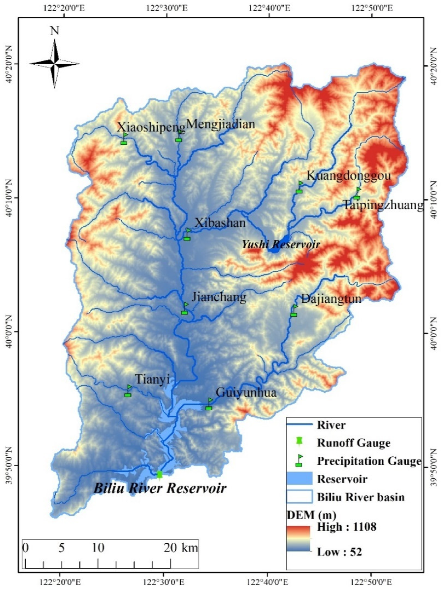
Figure 1. The location of precipitation gauges, runoff gauges, rivers, and boundaries in the Biliu River basin.
Sustainability 14 12201 g001
Figure 2. Flowchart of the uncertainty decomposition framework of this study.
Sustainability 14 12201 g002
Figure 3. The observed and simulated runoff of the calibration period (1982–1996).
Sustainability 14 12201 g003
Figure 4. The observed and simulated runoff of the validation period (1997–2011).
Sustainability 14 12201 g004
Figure 5. The SWAT model parameters’ uncertainty for the reference periods.
Sustainability 14 12201 g005
Figure 6. The uncertainty range of the precipitation change is shown for the four seasons.
Sustainability 14 12201 g006
Figure 7. (a) The Tmax for the 2050s and 2080s under the RCP4.5 and RCP8.5 scenarios based on 6 GCMs compared with the reference period (1980–2004). Lower and upper box boundaries indicate the 25th and 75th percentiles, respectively. The black lines and dots inside the box represent the median and mean value, respectively. The lower and upper whiskers indicate the 10th and 90th percentiles, respectively. (b) The T-min for the 2050s and 2080s under the RCP4.5 and RCP8.5 scenarios based on 6 GCMs compared with the reference period (1980–2004). Lower and upper box boundaries indicate the 25th and 75th percentiles, respectively. The black lines and dots inside the box represent the median and mean value, respectively. The lower and upper whiskers indicate the 10th and 90th percentiles, respectively.
Sustainability 14 12201 g007
Figure 8. (a) The ET for the 2050s and 2080s under the RCP4.5 scenario based on 6 GCMs compared with the reference period (1980–2004). Lower and upper box boundaries indicate the 25th and 75th percentiles, respectively. The black lines and dots inside the box represent the median and mean value, respectively. The lower and upper whiskers indicate the 10th and 90th percentiles, respectively. (b) The ET for the 2050s and 2080s under the RCP8.5 scenario based on 6 GCMs compared with the reference period (1980–2004). Lower and upper box boundaries indicate the 25th and 75th percentiles, respectively. The black lines and dots inside the box represent the median and mean value, respectively. The lower and upper whiskers indicate the 10th and 90th percentiles, respectively.
Sustainability 14 12201 g008aSustainability 14 12201 g008b
Figure 9. (a) The runoff in the 2050s and 2080s under the RCP4.5 scenario based on 6 GCMs compared with the reference period (1980–2004). Lower and upper box boundaries indicate the 25th and 75th percentiles, respectively. The black lines and dots inside the box represent the median and mean value, respectively. The lower and upper whiskers indicate the 10th and 90th percentiles, respectively. (b) The runoff in the 2050s and 2080s under the RCP8.5 scenario based on 6 GCMs compared with the reference period (1980~2004). Lower and upper box boundaries indicate the 25th and 75th percentiles, respectively. The black lines and dots inside the box represent the median and mean value, respectively. The lower and upper whiskers indicate the 10th and 90th percentiles, respectively.
Sustainability 14 12201 g009aSustainability 14 12201 g009b
Figure 10. The CIV values of hydrological climate-impact projections.
Sustainability 14 12201 g010
Figure 11. The SNR values of hydrological climate-impact projections.
Sustainability 14 12201 g011
Figure 12. The contribution of uncertainty sources to the runoff in the 2050s and 2080s.
Sustainability 14 12201 g012
Table 1. Description of CMIP5 climate models and scenarios.
Climate ModelsCountryResolutionScenarios
ACCESS1.0Australia1.88° × 2.48°RCP4.5, RCP8.5
BCC-CSM1.1(m)China1.13° × 1.13°RCP4.5, RCP8.5
CESM1(BGC)USA1.3° × 0.9°RCP4.5, RCP8.5
CESM1(CAM5)USA1.3° × 0.9°RCP4.5, RCP8.5
CMCC-CMItaly0.75° × 0.75°RCP4.5, RCP8.5
MPI-ESM-MRGermany1.88° × 1.88°RCP4.5, RCP8.5
Table 2. The selected SWAT model parameters.
ParameterDefinitionMinMax
CN2Initial SCS runoff curve number for moisture condition 0.75 1.25
SURLAGSurface runoff lag coefficient 1.00 23.98
LAT_TTIMELateral flow converge coefficient0.01 179.92
ESCOSoil evaporation compensation factor0.01 1.00
GW_DELAYThe delay time0.37 500.00
ALPHA_BFBaseflow alpha factors (days)0.00 1.00
GWQMNThreshold depth of water in the shallow aquifer required for return flow to occur0.41 499.72
SFTMPSnowfall temperature−5.00 5.00
SMFMXMelt factor for snow 1.50 8.00
TIMPSnowmelt temperature lag factor0.01 1.00
Table 3. The multiple liner regression coefficients for runoff (R mm year−1) with maximum temperature (Tmax °C), minimum temperature (Tmin °C), precipitation (P mm year−1) and ET (mm year−1) in a multiple linear regression model (R = a1 Tmax + b1 Tmin + c1 P+ d1 ET + e1). p is the significance level: *** p < 0.001, ** p < 0.01, * p < 0.05.
Modelsa1b1c1d1e1R2
ACCESS1-0_RCP4522.75−21.400.92 ***−0.97 ***−197.62 **0.96
ACCESS1-0_RCP8561.0523.890.97 ***−0.86−1284.580.75
BCC-CSM1.1(m)_RCP4520.96−15.300.85 ***−0.81 ***−237.050.92
BCC-CSM1.1(m)_RCP8517.26−13.920.84 ***−0.76 **−205.540.93
CESM1(BGC)_RCP4528.98−25.770.86 ***0.21 ***−209.880.93
CESM1(BGC)_RCP8581.42−38.460.99 ***−0.5−1370.22 ***0.86
CESM1(CAM5)_RCP4518.15−17.340.90 ***−0.93−153.060.96
CESM1(CAM5)_RCP8522.13−20.340.87 ***−0.77 ***−265.730.96
CMCC-CM_RCP455.9218.260.62 ***−0.53−248.500.75
CMCC-CM_RCP8515.40−14.670.68 ***−0.45 *−235.240.87
MPI-ESM-MR_RCP4529.52−24.950.88 ***−1.02 ***−224.860.94
MPI-ESM-MR_RCP8524.93−15.040.77 ***−0.65 **−348.450.90
Publisher’s Note: MDPI stays neutral with regard to jurisdictional claims in published maps and institutional affiliations.