Article

Predicting Monthly Runoff of the Upper Yangtze River Based on Multiple Machine Learning Models

1
State Key Laboratory of Water Resources and Hydropower Engineering Science, Wuhan University, Wuhan 430072, China
2
Institute for Water-Carbon Cycles and Carbon Neutrality, Wuhan University, Wuhan 430072, China
3
Chongqing Institute of Green and Intelligent Technology, Chinese Academy of Sciences, Chongqing 400714, China
4
Hubei Key Laboratory of Intelligent Yangtze and Hydroelectric Science, China Yangtze Power Co., Ltd., Yichang 443000, China
*
Authors to whom correspondence should be addressed.
Sustainability 2022, 14(18), 11149; https://doi.org/10.3390/su141811149
Submission received: 27 July 2022 / Revised: 28 August 2022 / Accepted: 2 September 2022 / Published: 6 September 2022

Abstract

:
Accurate monthly runoff prediction is significant to extreme flood control and water resources management. However, traditional statistical models without multi-variable input may fail to capture runoff changes effectively due to the dual effect of climate change and human activities. Here, we used five multi-input machine learning (ML) models to predict monthly runoff, where multiple global circulation indexes and surface meteorological indexes were selected as explanatory variables by the stepwise regression or copula entropy methods. Moreover, four univariate models were adopted as benchmarks. The multi-input ML models were tested at two typical hydrological stations (i.e., Gaochang and Cuntan) in the Upper Yangtze River. The results indicate that the LSTM_Copula (long short-term memory model combined with copula entropy method) model outperformed other models in both hydrological stations, while the GRU_Step (gate recurrent unit model combined with stepwise regression method) model and the RF_Copula (random forest model combined with copula entropy method) model also showed satisfactory performances. In addition, the ML models with multi-variable input provided better predictability compared with four univariate statistical models, and the MAPE (mean absolute percentage error), RMSE (root mean square error), NSE (Nash–Sutcliffe efficiency coefficient), and R (Pearson’s correlation coefficient) values were improved by 5.10, 4.16, 5.34, and 0.43% for the Gaochang Station, and 10.84, 17.28, 13.68, and 3.55% for the Cuntan Station, suggesting the proposed ML approaches are practically applicable to monthly runoff forecasting in large rivers.

1. Introduction

Flood is a complex interplay of hydrology, climate, and human management, and it is destructive to infrastructure, agriculture, and socioeconomic systems [1,2]. Yet water resource management, such as water conservation, flood control, and reservoir operation, relies heavily on accurate streamflow prediction [3,4,5]. In addition, streamflow is affected by multiple variables, such as precipitation, surface temperature, solar radiation, and atmospheric circulation, presenting the compound characteristics of strong nonlinearity, high uncertainty, and spatiotemporal variability [6,7,8,9]. Consequently, the high accuracy of monthly flood and streamflow prediction involving multiple impact factors has been emphasized urgently.
Different runoff prediction models have been proposed. Generally, these models can be divided into process-driven and data-driven models [5,10]. Process-driven models based on the physical conception have some modeling conventions, such as data limitations and uncertainty for the initial conditions, process parameterizations, and computational constraints [11,12]. Among the data-driven models, traditional univariate statistical models only require runoff input [13], such as the autoregressive moving average (ARMA) model, mean generating function (MGF), nearest neighbor bootstrapping regressive (NNBR) model, and grey model (GM) [14,15,16,17]. Statistical models have been used extensively to capture the stationary and linear links in time series but may not be appropriate for predicting nonstationary and nonlinear runoff. Machine learning (ML) models [3], which are outstanding at handling nonlinear data, have been widely applied in hydrological prediction, including artificial neural networks (ANNs), support vector machine (SVM), gradient boosted decision tree (GBDT), etc. Derived from the biological neurons, ANNs build mapping with a vast amount of parameters to match the mapping between observation and prediction. Many new ANNs have arisen to provide more satisfactory solutions to time series forecasting problems, including the long short-term memory model (LSTM) and gate recurrent unit model (GRU). Due to the weakness of the conventional ANN for long-term dependencies, LSTM is constructed to improve the defects [18]; GRU has a much simpler structure and thus needs less calculation than LSTM. GBDT and random forests (RF) have been proven to be distinguished predictive models in many regression tasks with an ensemble of decision trees [19,20]. The SVM, founded on the theory of statistical learning as well as the principle of structural risk minimization [21], can address problems with limited samples, nonlinearity, and impartibility in low-dimensional space.
Unlike traditional regression models, ML models have considerably upgraded the mid-to-long-term forecasting performance of highly nonlinear streamflow time series. Many previous studies [5,11,13,22] have shown that the traditional statistical models’ performances stagnated at 15–20% in terms of mean absolute percentage error, demonstrating the urgency of adopting new ML models. However, since there is no absolute optimal model for forecasting monthly runoff, it is necessary to use multiple ML models and compare their performances.
The identification of input variables is a critical part of the data-driven models. It is difficult to determine a suitable set of model inputs because of the complexity of the causes and the time lag in the runoff response to large-scale atmospheric circulation and surface meteorological variables [23]. Many teleconnection climate indexes [3] have been considered as alternative candidate predictive variables, including atmospheric circulation index, SST indexes, and other indexes, such as the total sunspot number index, Pacific decadal oscillation index, North Atlantic triple Index, etc. Besides, the antecedent runoff and other surface meteorological factors, such as precipitation, air pressure, temperature, wind speed, etc., are firmly connected on the grounds of physical links [24]. The methods used in variable selection are principally the correlation coefficient method, stepwise regression analysis, principal component analysis (PCA) [4], mutual information (MI), and partial mutual information (PMI) [25,26]. Among the various variable selection methods, the correlation coefficient method and the stepwise regression method are widely applied due to their simplicity and clarity [23]. Furthermore, copula entropy, a novel entropy concept defined by Ma and Sun [27,28] in 2008, is able to calculate the full-order correlations among variables and handle the redundant inputs directly. Copula has been applied in multivariate modeling with joint distributions, where two divisions, entropy copula and copula entropy, have been broadly employed in the hydrological study [28,29]. The entropy copula is mainly used in constructing a dependence structure with marginal probability distribution constraints. In addition, the copula entropy, which is outstanding in dependence analysis, has been used to study the variability of climate and hydrological variables, mostly precipitation, temperature, and streamflow [30]. However, the copula entropy method is rarely applied in nonlinear dependence measurement among large-scale circulations and streamflow in monthly runoff prediction, highlighting the importance of incorporating this method into data-driven model input variable identification [31].
The climate in the Upper Yangtze River Basin (UYRB) in China is complex due to complex topography and the interplay among diverse circulation systems (for instance, the East Asia monsoon, Indian monsoon, Australian monsoon, mid-latitude westerlies, and plateau monsoon) as well as the water conservancy projects construction [32]. The Three Gorges Reservoir (TGR), situated in the UYRB, is the world’s largest hydropower station in terms of installed capacity [33,34,35], and the power production and the overall profits of which are heavily reliant on the upstream flows. Located in the lower reaches of the confluence of the Dadu River and Min River [36,37], the Gaochang Station is the outlet of the Min River basin, controlling 13.46% of the drainage area and 19.86% of the annual flow in the UYRB [38]. The Cuntan Station is located in Chongqing City, where the Jialing River meets the Yangtze River [39], and it controls about 60% of the water in the UYRB. Therefore, the monthly runoff prediction study on the Gaochang Station and Cuntan Station is not only related to the operation of TGR but also vital to human life and property in the middle and lower reaches.
In this study, we aimed to improve the accuracy of monthly streamflow prediction in the UYRB for the power generation in the Three Gorges Reservoir and the long-term flood management in the middle and lower reaches. Furthermore, the role of multi-variable inputs and the choice and performance of different predictive models are of particular interest to us. Therefore, five multi-input ML models were employed to make the best use of available data, combined with the stepwise regression method or copula entropy method to select input variables with different time lags. The ML models were carried out in two typical hydrological stations of the UYRB, and the detailed case study is presented in the following sections.

2. Methods

2.1. Study Area and Data

The mainstream of the UYRB is 4529 km long, and it charges a watershed of 1,000,000 km2, which covers the region from 24.30° N–35.45° N to 90.33° E–112.04° E and represents 58.9% of the entire region of the Yangtze River [39,40]. Most of the regions in the UYRB are warm and moist, influenced by subtropical monsoon [24]. The mean annual streamflow varies between 700 and 2400 m3/s, and the Three Gorges Station in the mainstream reached an annual runoff of 16,427 m3/s in 1965, and the Zipingpu Station in the Min River was less than 265 m3/s in 2006 [41]. Here, two critical hydrological stations—Gaochang and Cuntan in the UYRB were examined (Figure 1).
Monthly streamflow data of the Gaochang and Cuntan stations from January 1961 to December 2018 were collected in our study. One hundred and thirty monthly global circulation indexes within the same timeframe as the streamflow observations were downloaded from the National Climate Center of the China Meteorological Administration (http://cmdp.ncc-cma.net (accessed on 20 June 2022)), including 88 atmospheric circulations, 26 SST indexes, and 16 other indexes. Moreover, two meteorological stations near the selected hydrological stations were considered with complete monthly observations spanning the period of 1961–2018, including air pressure, average temperature, maximum temperature, minimum temperature, relative humidity, wind speed, and daylight hours, which were supplied by the China Meteorological Data Network (https://data.cma.cn/ (accessed on 20 June 2022)).
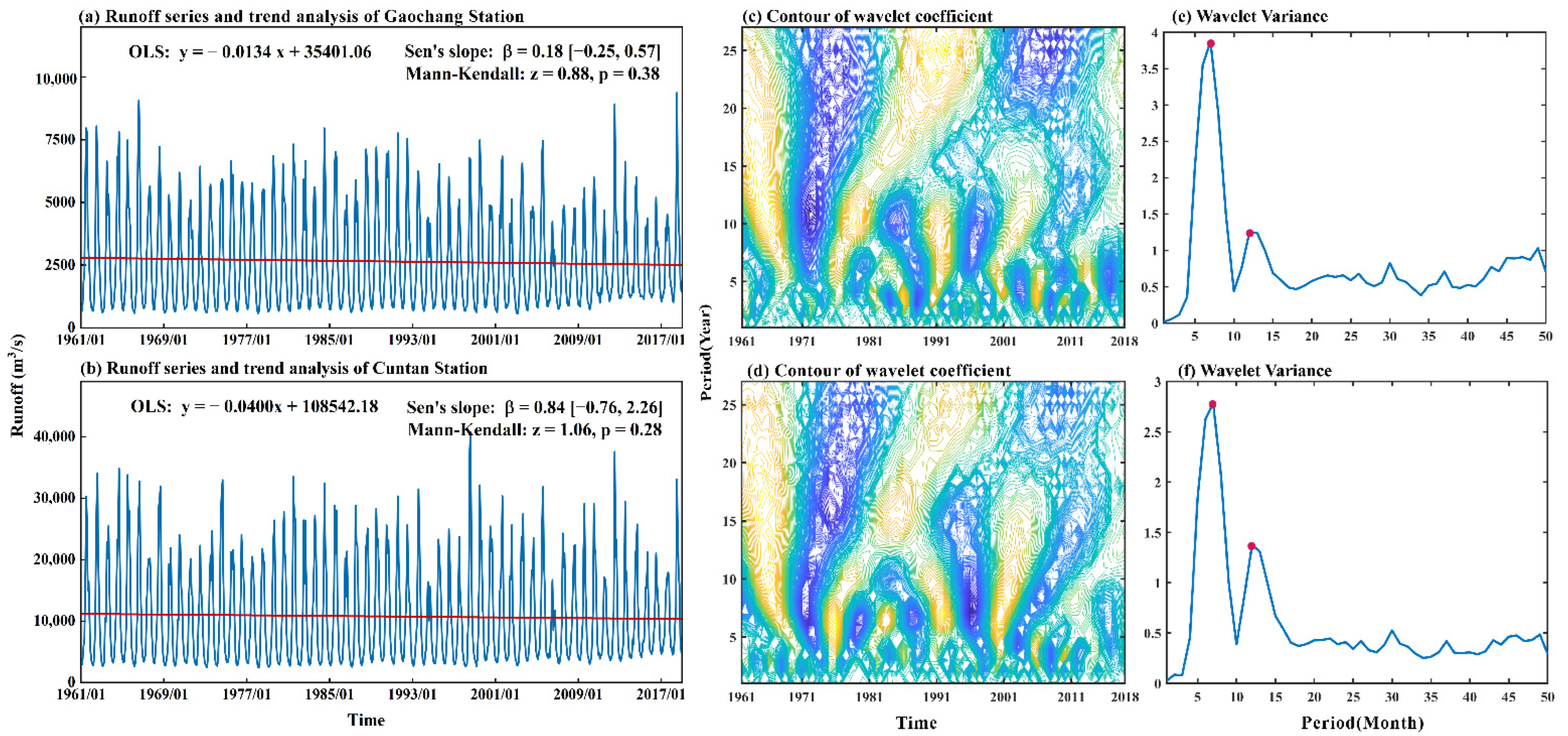
The trend, change point, and periodicity of the monthly streamflow in the Gaochang and Cuntan stations were detected (Figure 2). No statistically significant trend (at a 5% significance level) was observed by the non-parametric Mann–Kendall test [42] and Sen’s slope [43], with a p-value of 0.38 at Gaochang Station and 0.28 at Cuntan Station. The most probable change point was found to be NO. 593 (May 2010) at Gaochang Station and NO. 448 (April 1998) at Cuntan Station by Pettitt’s Test [44], but the results did not indicate statistical significance. The Morlet wave analysis method [45] was used to analyze the periodic characteristics of the annual average and monthly runoff series. The 10–13 yearsoscillation period was most notable, the 3–5 years period was relatively notable at Gaochang Station, and the principal period and the second period of monthly runoff was found to be seven months and twelve months. While at the Cuntan Station, the 7–10 years oscillation period was most notable, and the principal period was found to be seven months with the maximum value of wavelet variance.
Based on the analysis above, the data series was divided into two periods, i.e., January 1961–December 2008 for model training and January 2009–December 2018 for testing. Owing to the lag effect of climate causes on streamflow and the periodicity of the monthly runoff in Gaochang and Cuntan stations, 1–12 months were considered as the different lag periods when selecting the input factors in this study. Normalization of the climate and runoff data in training and testing periods was applied to refrain from the numerical problem.

2.2. Variable Selection

The Pearson’s correlation coefficient, stepwise regression, and copula entropy methods were applied to select input variables with different time lags. For example, to predict the runoff in January 2010, data from the previous 1 to 12 months were selected as forecast variables, and Pearson’s correlation coefficient analysis first identified the top 150 variables; then the multiple stepwise regression analysis or copula entropy analysis was carried out to select the most relevant variables with the significance test.

2.2.1. Pearson’s Correlation Coefficient

Pearson’s correlation coefficient assesses the relationship between monthly runoff and explanatory variables. The coefficient R is estimated by [46]:
R = i = 1 n ( x i x ¯ ) ( y i y ¯ ) i = 1 n ( x i x ¯ ) 2 i = 1 n ( y i y ¯ ) 2

2.2.2. Stepwise Regression

Stepwise regression is a multivariate regression analysis method that plays an integral role in hydrological research and modeling. The multiple stepwise regression adds the most significant variables one by one [11]. After adding a new variable at each step, an F-test is performed to determine whether certain variables will be removed without remarkably increasing the sum of squared residuals.

2.2.3. Copula Entropy

The entropy of the copula function, CE, was used to evaluate the dependence among variables [27]. X 1 and   X 2 are random variables with marginal functions F ( x 1 ) , F ( x 2 ) , and U 1   = F ( x 1 ) , U 2 = F ( x 2 ) , u 1 and u 2 represent a particular value of U 1 and U 2 . The definition of CE is as follows:
H C ( U 1 , U 2 ) = 0 1 0 1 c ( u 1 , u 2 ) log c ( u 1 , u 2 ) d u 1 d u 2
where   c ( u 1 , u 2 ) is the copula probability density function and is identical to C ( u 1 , u 2 ) u 1 u 2 .
Mutual information (MI) is denoted as [47]:
T ( X 1 , X 2 ) = H ( X 1 ) + H ( X 2 ) H ( X 1 , X 2 ) = H C ( U 1 , U 2 )
MI can detect nonlinear correlations between target input and output [48]. However, this method cannot handle the redundant inputs directly [49], and to deal with this issue, Sharma [47] proposed partial mutual information (PMI). The PMI can be derived with the CE method:
P M I = f X Y ( x , y ) ln [ f X Y ( x , y ) f X ( x ) f Y ( y ) ] d x d y = H C ( x , y )
Fernando and May [50] suggested the Hampel test as the termination criteria:
Z i = d i 1.4826 d i ( 50 ) · d i = | C E i C E ( 50 ) |
where: Z i —Hampel distance; 1.4826—normalization variables; d i ( 50 ) —median of d i ; C E i —the copula entropy of the i th variables; C E ( 50 ) —median CE values for variables set; Based on the 3σ principle, when the Hampel distance is above 3, add the candidates to the input.
In this paper, the R (R Core Team 2020) package ‘copent’ (https://github.com/majianthu/copent (accessed on 20 June 2022)) was applied, which implements the nonparametric method for estimating CE [27].

2.3. Prediction Models

The application of LSTM, GRU, GDBT, and RF relies on Python 3.9 with the “Scikit-Learn” package, and the libsvm package in MATLAB R2020 (a) (https://www.csie.ntu.edu.tw/~cjlin/libsvm/index.html (accessed on 20 June 2022)) was employed in the SVR prediction.

2.3.1. Long Short-Term Memory (LSTM)

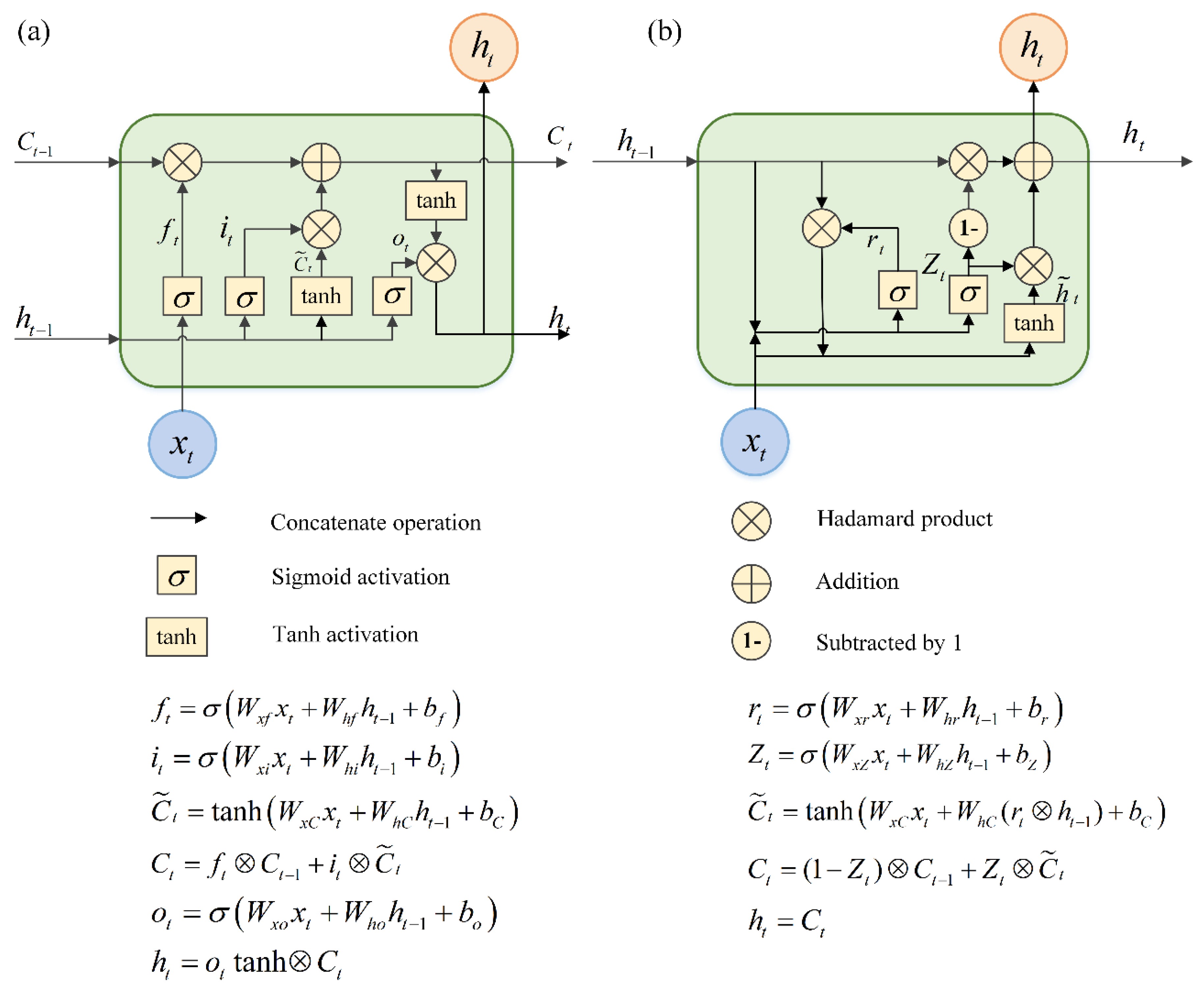
The LSTM model comprises the input, hidden, recurrent, and output layers [48]. The memory block in the recurrent layer facilitates the interaction between the three layers, which involves multiple memory cells and three multiplier units [49]. The fundamental construction of an LSTM memory cell is displayed in Figure 3a. These three gates serve as filters [50]: The forget gate determines what message will be excluded, the input gate sets what new message will be collected, and the output gate specifies the output message from the cell condition [51].

2.3.2. Gate Recurrent Unit (GRU)

GRU networks were proposed to modify LSTM networks [52] with a simpler structure and faster speed. The fundamental construction of the GRU cell is displayed in Figure 3b. The hidden state ( h t ) and cell state ( C t ) are merged in the GRU. There are two control gates in the cell: the update gate ( Z t ) and the reset gate ( r t ) [53]. The update gate controls the extent to which the message from the prior step t 1 will be passed to the current step t [48]. The reset gate determines how much information of the prior state is written into the current candidate set C ˜ t .

2.3.3. Gradient Boosted Decision Tree (GBDT)

A GBDT regression model is constructed using various decision trees (DTs) [54]. In every iteration, the latest DT is trained according to the residuals of the prior DTs based on the negative gradient, which has been confirmed to be an efficient, precise, low-bias algorithm [18,55]. This study uses the Gaussian distribution as a loss function to minimize the squared error.

2.3.4. Random Forest (RF)

RF is an ensemble of the decision tree model based on the bagging method [54]. As a white-box model, RF samples the raw data and generates many training samples by bootstrapping. The bagging method may address the overfitting problem of forecasting models [20,56].

2.3.5. Support Vector Regression (SVR)

Support vector regression (SVR) is employed in support vector machine (SVM) for regression tasks [57,58]. Based on Lagrange binary theorem [22], the SVR model tacitly transforms the original, low-dimension input into high-dimension space. In our research, the nonlinear radial basis function (RBF) was applied as the kernel function since it has demonstrated exemplary performance in predicting nonlinear runoff data for SVR [59].

2.4. Metrics of Performance Evaluation

Four metrics were applied to evaluate the performance of the forecasting models, including the mean absolute percentage error (MAPE), root mean square error (RMSE), Nash–Sutcliffe efficiency coefficient (NSE), and Pearson’s correlation coefficient (R), which are specified as follows:
M A P E = 1 n × i = 1 n | Y i Y ^ i Y i | × 100 %
R M S E = 1 n × i = 1 n ( Y ^ i Y i ) 2
N S E = 1 i = 1 n ( Y i Y ^ i ) 2 i = 1 n ( Y i Y a v g ) 2
R = i = 1 n [ ( Y i Y a v g ) ( Y ^ i Y ^ a v g ) ] i = 1 n ( Y i Y a v g ) 2 i = 1 n ( Y ^ i Y ^ a v g ) 2
where n is the amount of data, Y i and Y ^ i represent the i th observation and prediction, and Y a v g and Y ^ a v g are the average of all the observation and prediction.
MAPE and RMSE can evaluate models’ performance, especially high streamflows; NSE is used to test the deviation of a forecasting model, ranging from to 1 [60]; R is adapted to evaluate the linear correlation between observation and prediction. Models with larger R and NSE values or smaller MAPE and RMSE values indicate better predictive performance [61].

2.5. Model Calculation Scheme

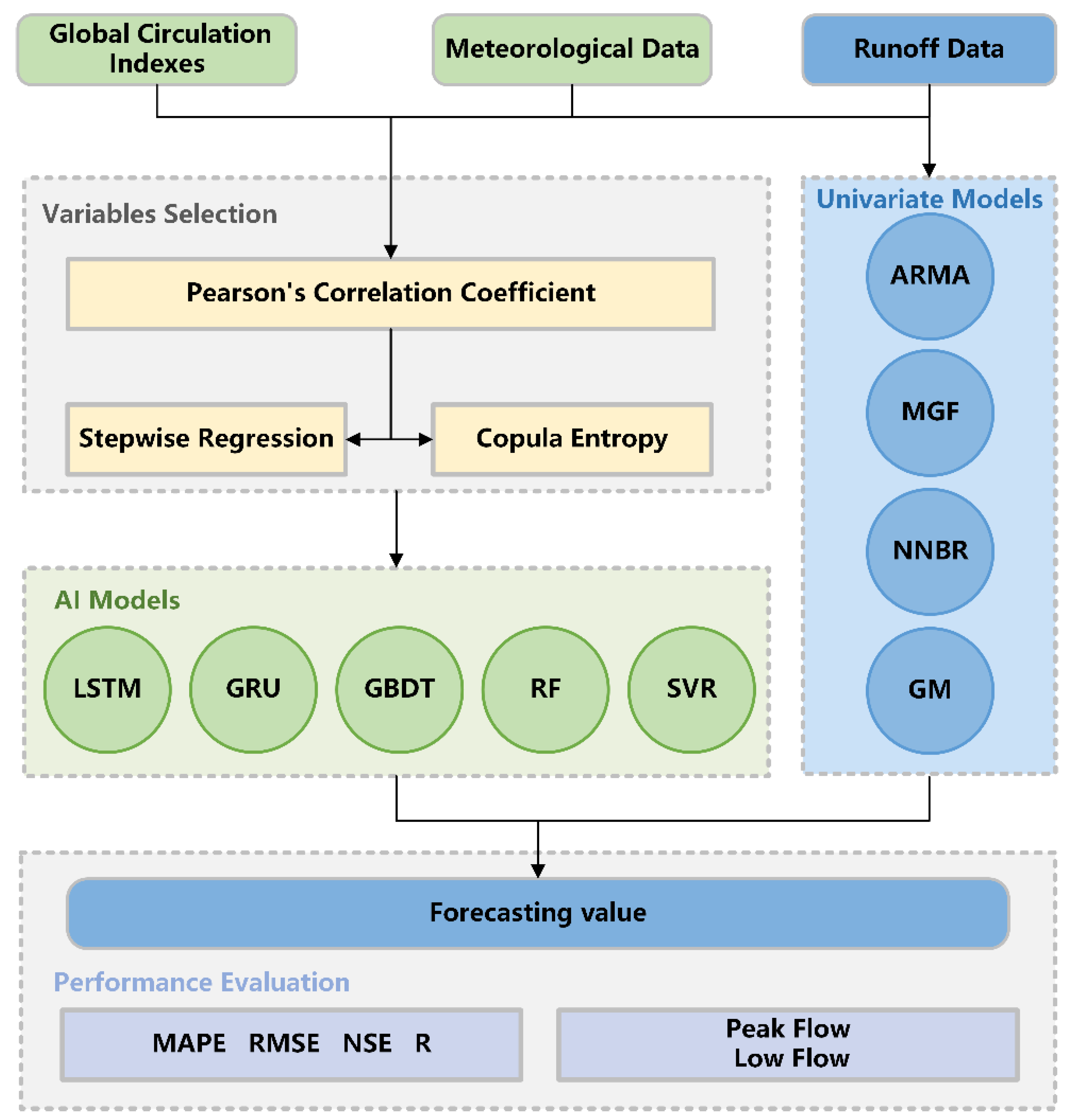
Cause-driven multivariate forecasting models reflect the relationship between variables and forecast elements regarding runoff causation [18]. The selection of variables and forecast models are crucial when applying this approach. The model calculation scheme is shown below (Figure 4).
First, the essential variables were chosen as the model input set. The candidate predictive variables include one hundred thirty global circulation indexes, eight surface meteorological data, and the antecedent runoff (Table S1). The total number of variables is 139 × 12 , considering the lag time of 1–12 months. Subsequently, the selected variables by different methods were input into five ML models, and four classical univariate time series models were used as benchmarks. Last, four indicators were used to measure the performance of the prediction models. Thus, the optimal monthly runoff prediction model and a few sub-optimal models were recommended by comparing a weighted average score of four metrics for a specific station.

3. Results

3.1. Variable Selection

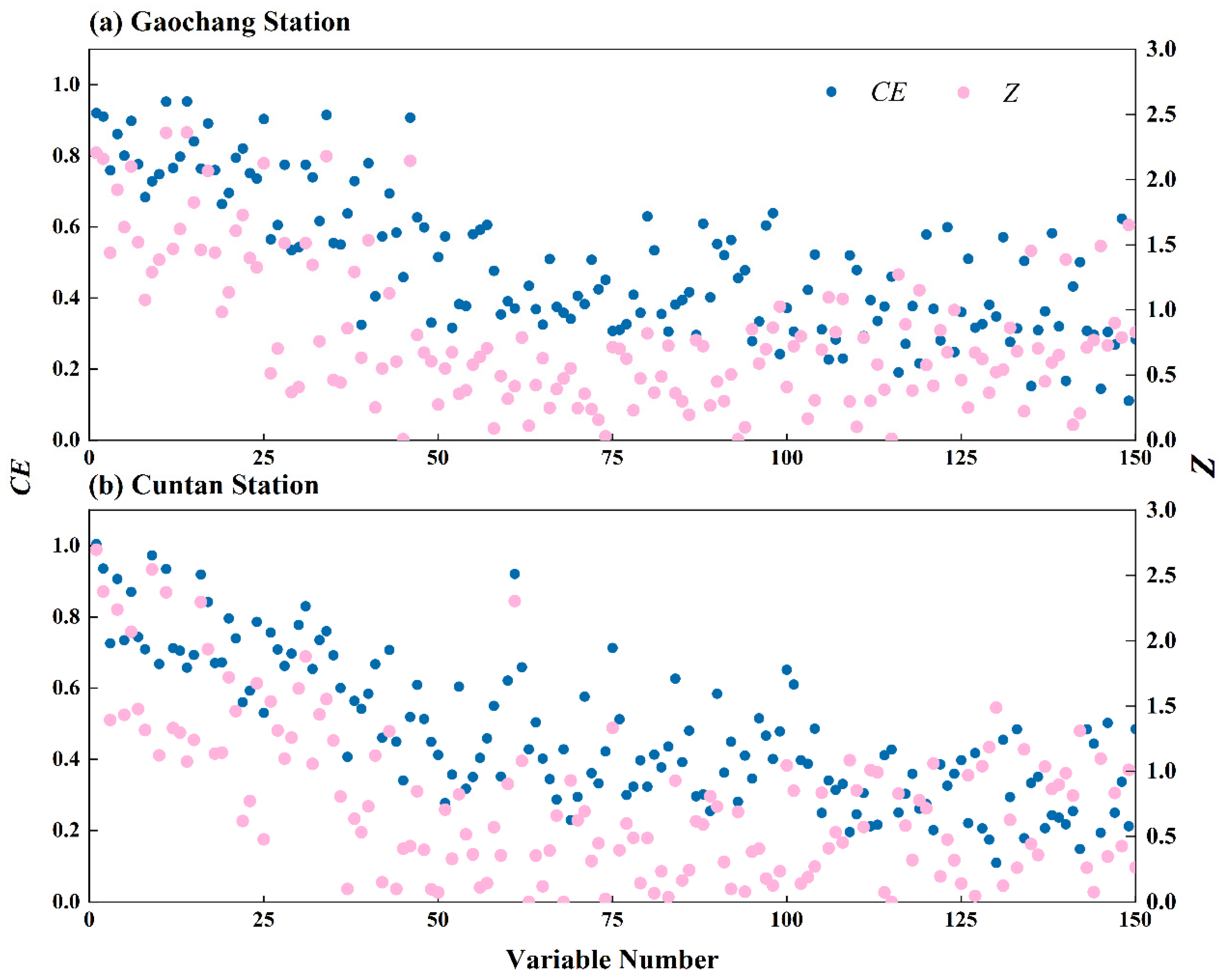
The top 150 variables were first identified by Pearson’s correlation coefficient analysis, followed by the multiple stepwise regression analysis or copula entropy analysis to select the most relevant variables. The calculated copula entropy and Z values of the first 150 variables are shown in Figure 5. Z represents the CE value after the Hample test, which fluctuates more than CE at both the Gaochang Station and the Cuntan Station. Based on the 3σ criterion, when Z is greater than 3, the candidate variable has a significant entropy value and can be added to the input set. However, none of the variables had a Z value greater than 3. Hence, a lower confidence level was considered in this paper and the top ten variables in terms of Z value were identified as an input set for the forecasting models. To keep the number of variables in the input set consistent, the top ten variables were selected in stepwise regression analysis after the multicollinearity testing and correction.
The variables selected by stepwise regression and copula entropy are listed in Table 1. For the Gaochang Station, average temperature, runoff, and maximum temperature were selected by stepwise regression and copula entropy methods. The stepwise regression method selected more global circulation variables, such as the northern hemisphere polar vortex central intensity index, Tibet Plateau region 1 index, Asia polar vortex area index, and so on; while the copula entropy method selected more ground meteorological variables. Most of the variable’s lag was 1 month, followed by 12 months and 6 months, which is synchronous with the natural period of the water cycle. For the Cuntan Station, the maximum temperature was the most significant variable selected both by the stepwise regression method and the copula entropy method. Besides, runoff with 1 month, 6 months, and 12 months’ time lag were selected, indicating a strong autocorrelation in streamflow. Likewise, the tepwise regression tended to select more global circulation variables than the Copula Entropy method at the Cuntan Station.

3.2. Model Structure and Parameter Selection

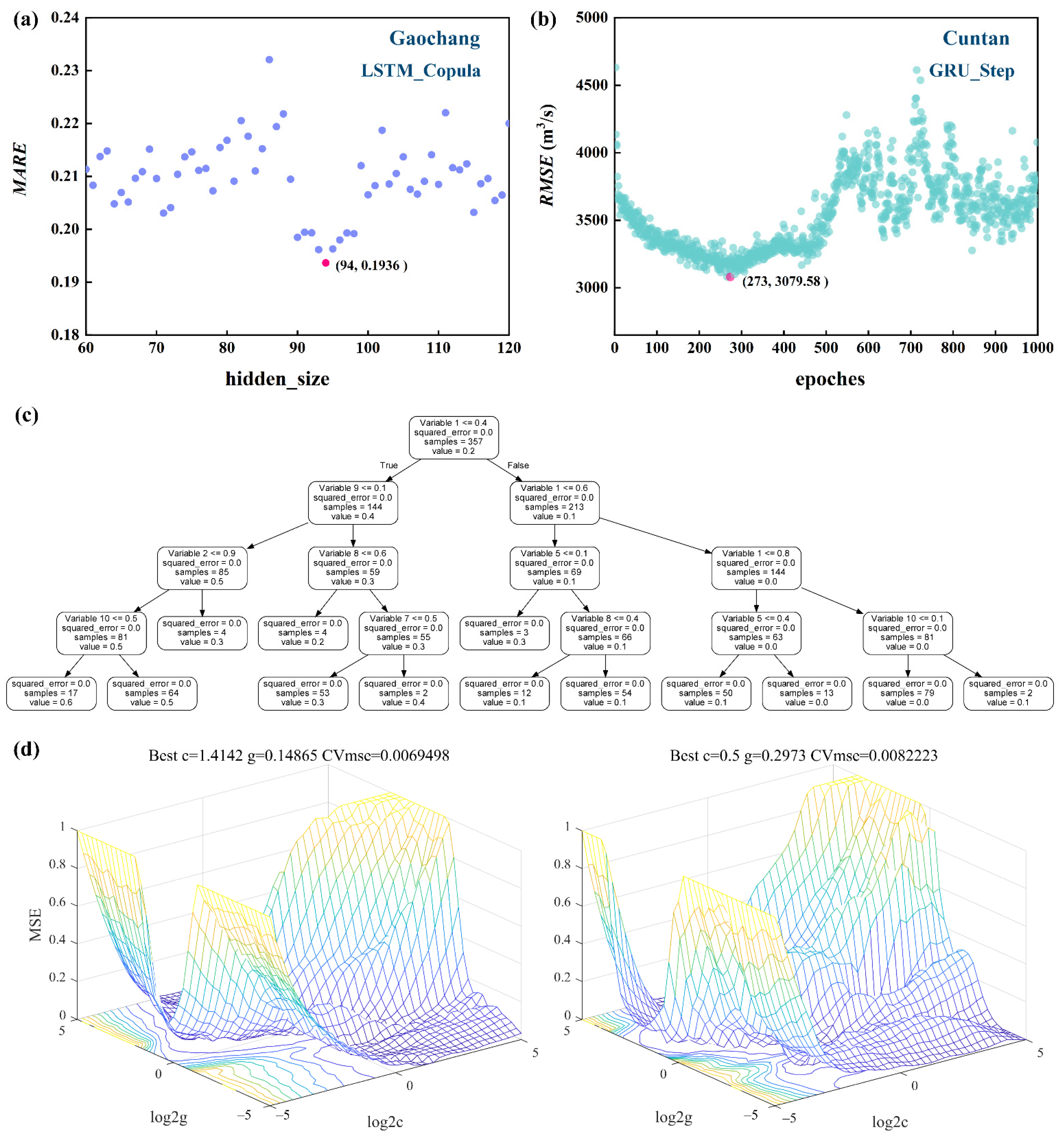
In the development of LSTM and GRU, the num_layers and batch_size were set to 2 and 12, separately, and the hidden_size from 60 to 120 was examined to identify the optimal networks. In addition, the epochs were set as 1000 times, and the learning rate was set as 0.0005, while the best models were evaluated by minimum MARE in the testing stage. For the Gaochang Station, the optimal parameters (hidden_size and epoches) of the LSTM_Step model, LSTM_Copula model, GRU_Step model, and GRU_Copula model were (112, 862), (94, 977), (68, 562), and (75, 788) respectively. For the Cuntan Station, the optimal parameters of the LSTM_Step model, LSTM_Copula model, GRU_Step model, and GRU_Copula model were (70, 357), (95, 488), (85, 273), and (106, 634). The parameter optimization process of hidden_size in the LSTM_Copula model at Gaochang Station was demonstrated in Figure 6a, where the model performance improved when the hidden_size was in a range of 90~100 but decreased when the hidden_size was more than 100. The performance of the GRU_Step model at the Cuntan Station was improved as the epochs increased but reduced when ephochs were larger than 330 (Figure 6b).
In the modeling with GDBT and RF, the hyperparameter setting is a key step, where randomized search and grid search were used sequentially. Firstly, the n_estimators (the number of decision trees), max_depth (the maximum depth of decision trees), min_samples_split (the minimum number of split samples), min_samples_leaf (the minimum sample size of the nodes), and max_features (the maximum sampling ratio) in the hyperparameter were set in a relatively wide range, and 200 random iterations were performed with 3-fold cross-validation using RandomizedSearchCV.py. Based on the result of the randomized search, a few values were selected in the nearby range, and each match was traversed through GridSearchCV.py to search for the optimal hyperparameter values (Figure 6c). For the Gaochang Station, the optimal hyperparameters of the GDBT_Step model, GDBT_Copula model, RF_Step model, and RF_Copula model are (230, 38, 9, 1, 2), (910, 50, 3, 2, 3), (380, 14, 11, 2, 4), (127, 28, 3, 2, 1) respectively. For the Cuntan Station, the optimal hyperparameters of the GDBT_Step model, GDBT_Copula model, RF_Step model, and RF_Copula model are (50, 35, 6, 1, 2), (100, 22, 11, 1, 2), (90, 46, 11, 2, 4), (270, 17, 2, 1, 3) respectively.
The grid search method of 3-fold cross-validation is applied to find the best values for cost (c) and gamma (g), two crucial parameters in the SVR model (Figure 6d). For the Gaochang Station, the optimal parameters of the SVR_Step model and SVR_Copula model are (1.41, 0.15), (0.50, 0.29), respectively. For the Cuntan Station, the optimal parameters of the SVR_Step model and SVR_Copula model are (3.0, 0.29), (6.0, 0.42) respectively.

3.3. Comparison of Various Models’ Performance

Among the ten models examined herein, the GBDT_Step and GBDT_Copula models achieved the best MAPE, RMSE, NSE, and R values in the training stage for the two stations (Table S2). In the testing period, the GRU_Copula model obtains the best MAPE values of 16.68%, and the LSTM_Copula model performs better than other models in RMSE, NSE, and R for the Gaochang Station. While for the Cuntan Station, the SVM_Step model obtains the best MAPE values of 13.98%, followed by LSTM_Copula of 14.44%; the RF_Copula model achieves the best RMSE values of 2616 m3/s, and LSTM_Copula accomplishes the best NSE and R values.
The copula entropy method had a more consistent performance effect across the months than the stepwise regression method, which was distinct in LSTM, GBDT, and SVR models (Figure S1). For the Gaochang Station, the LSTM_Copula model outperformed other models with better values among four evaluation metrics and a more robust effect on different months. For the Cuntan Station, models performed differently on different indicators, but LSTM_Copula, GRU_Step, and RF_Copula models performed better overall.
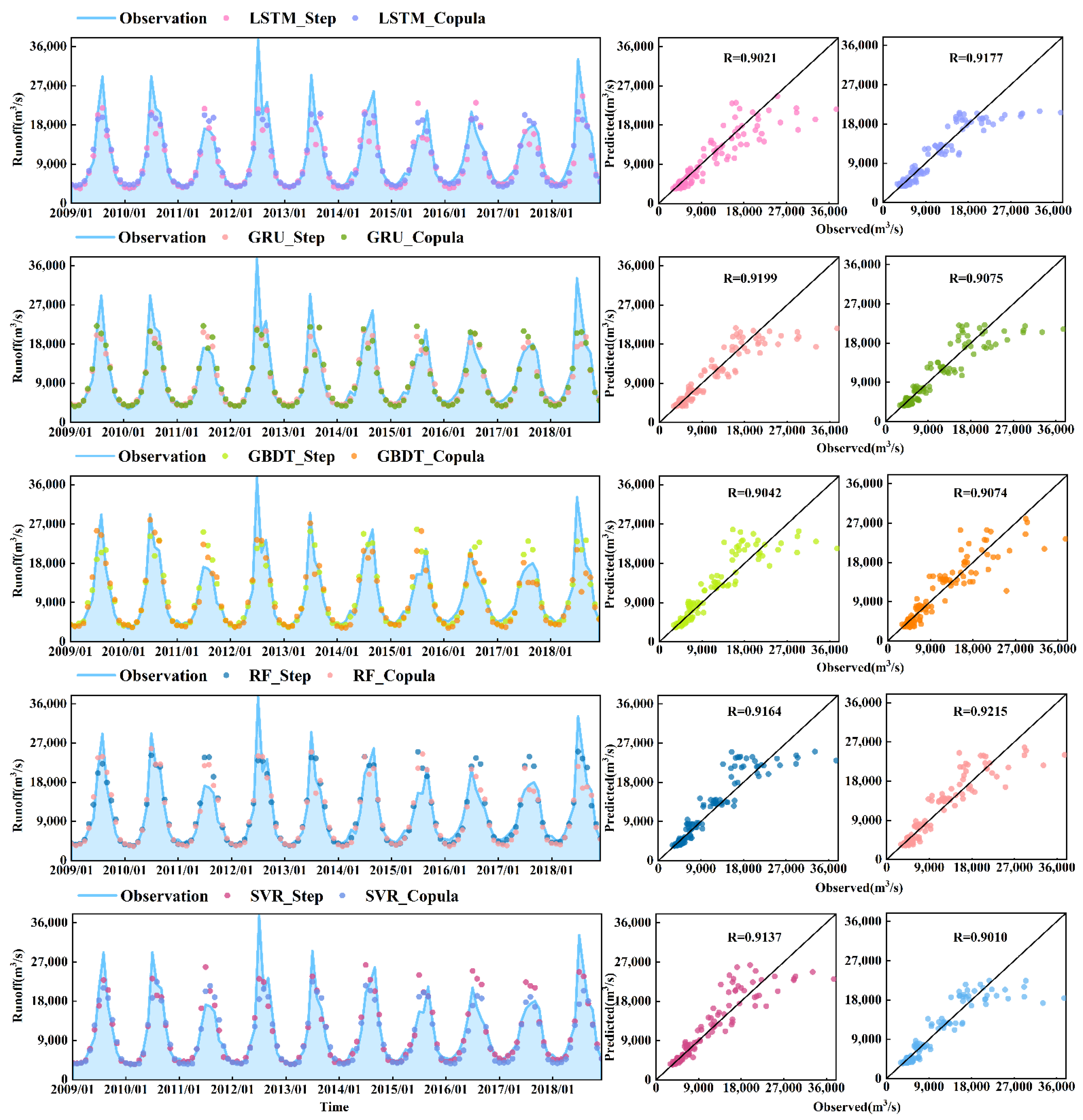
All the ML models could track the observed changes in the runoff series, manifesting the validity of the ML models (Figure 7 and Figure 8). For the Gaochang Station, GBDT and SVM models were superior to the other methods because the deviations between the observations and simulations were small, and the high flows above 6000 m3/s were better captured. In addition, the two selection methods did not show much difference when applied in the five ML models. For the Cuntan Station, GBDT and RF models outperformed other models from the denser results in the scatter plots; and the Copula method performed better in LSTM and SVR models. Given that the peak flows at two stations were not well predicted, the ten models need to be improved in simulating hydrological extremes.
To further illustrate the advantages of using multi-variable inputs for data-driven models, four classical univariate time series models were used as benchmarks: ARMA, MGF, NNBR, and GM (Table S3 and Figure S2). In the testing stage, the ARMA model outperformed other models with the best MAPE, RMSE, and NSE values for the Gaochang Station. In addition, the ARMA model had a more concentrated distribution of monthly average MAPE and NSE, while the MGF model outperformed on RMSE and R. For the Cuntan Station, the ARMA model achieved the best MAPE values of 14.39% and the best NSE of 0.84, while the MGF model outperforms the ARMA with an R-value of 0.96. Similarly, the ARMA model’s MAPE and NSE have more concentrated distributions than other univariate models, and the MGF model outperforms on RMSE and R. The same results can be found in univariate models where the observed and predicted values overlap and cluster.
Overall, the four univariate models did not predict the monthly streamflow well enough like the ML models. For the Gaochang Station, the univariate models’ MAPE ranged from 17.47~27.79%, the RMSE ranged from 715 to 887 m3/s, and the NSE ranged from 0.52~0.77, except that the evaluation metric R was relatively better with a range of 0.89~0.95, whereas the ML model’s MAPE ranged from 16.68~26.26%, the RMSE ranged from 691~844 m3/s, the NSE fluctuated from 0.58 to 0.78, the R fluctuated from 0.91~0.94, which illustrated the improvement of the ML model over the univariate model in terms of MAPE by 5.10, RMSE by 4.16, NSE by 5.34, and R by 0.43%. The evaluation of the four models was quite the same for the Cuntan Station, and the improvement of the ML model over the univariate model was more apparent, with MAPE by 10.84, RMSE by 17.28, NSE by 13.68, and R by 3.55%.
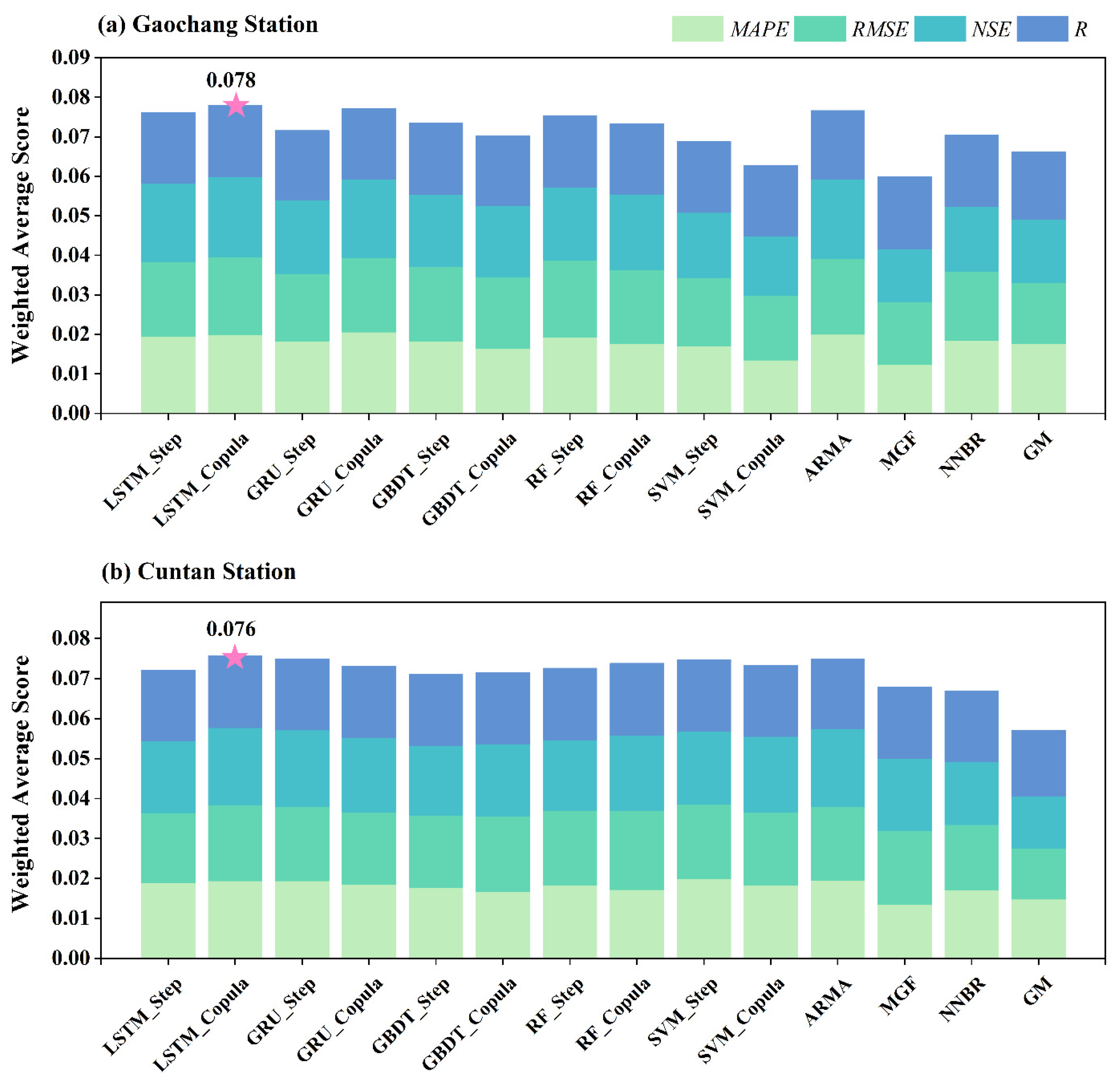
The performance of these 14 models was quantitatively compared based on the entropy weight method (Figure 9). Four evaluation metrics, MAPE, RMSE, NSE, and R, were considered comprehensively through the index weight and normalized value calculated by the entropy method, where MAPE and RMSE were negative metrics while R and NSE were positive metrics. It turned out that the index weights were close both in the Gaochang Station and the Cuntan Station, ranging from 0.249~0.251. The best weighted average score for the Gaochang Station was 0.0780 from the LSTM_Copula model, followed by the GRU_Copula with a score of 0.0771; while the lowest score was 0.0599 in the MGF model. For the Cuntan Station, the best weighted average score was 0.0758 in the LSTM_Copula model, while the lowest score was 0.0570 in GM. The weighted average performance score for the Gaochang Station differed significantly among these 14 models, whereas for the Cuntan Station, the ML models indicated a similar performance except for the LSTM_Step model, and there was a significant advantage compared with the univariate models, with an average improvement of 0.0093.

3.4. Accuracy of Peak Flow and Low Flow Forecasts

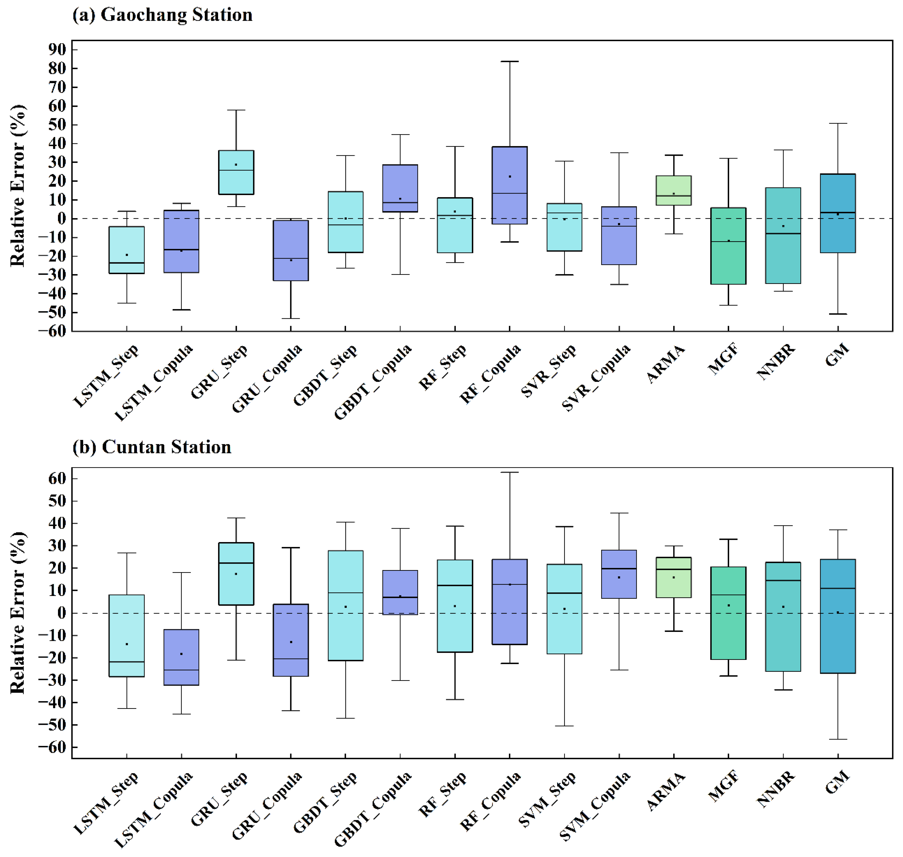
Generally, the peak flows were not captured well, and all models failed to capture the most severe peak flow (Figures S3 and S4). For the Gaochang Station, the peak flows in 2012 and 2018 were not captured by any of the ten ML models or the four univariate models (Figure S3). The observed peak flow in 2012 was 8921 m3/s, but the average predicted peak flow was only 5278 m3/s, which was even more inaccurate in 2018, with an observed peak flow of 9366 m3/s and a predicted value of 5314 m3/s. In other years, LSTM and GRU models tended to underestimate the peak flows to 9.58~14.34%, while GBDT, RF, and SVR tended to overestimate the peak flows to 4.94~12.50%. For the Cuntan Station (Figure S4), the GDBT_Copula model tracked the peak flow better than others in 2009, 2010, 2013, and 2017. The peak flow in 2012 was underestimated by all the ten ML models to an average of 41.06% and by the four univariate models to an average of 34.8%. The highest peak flow in 2018 was underestimated by the ten ML models to an average of 33.01% and by the four univariate models to an average of 29.85%. Besides, the peak flow in 2011 was overestimated by the ten ML models to an average of 31.51% and by the four univariate models to an average of 24.15%.
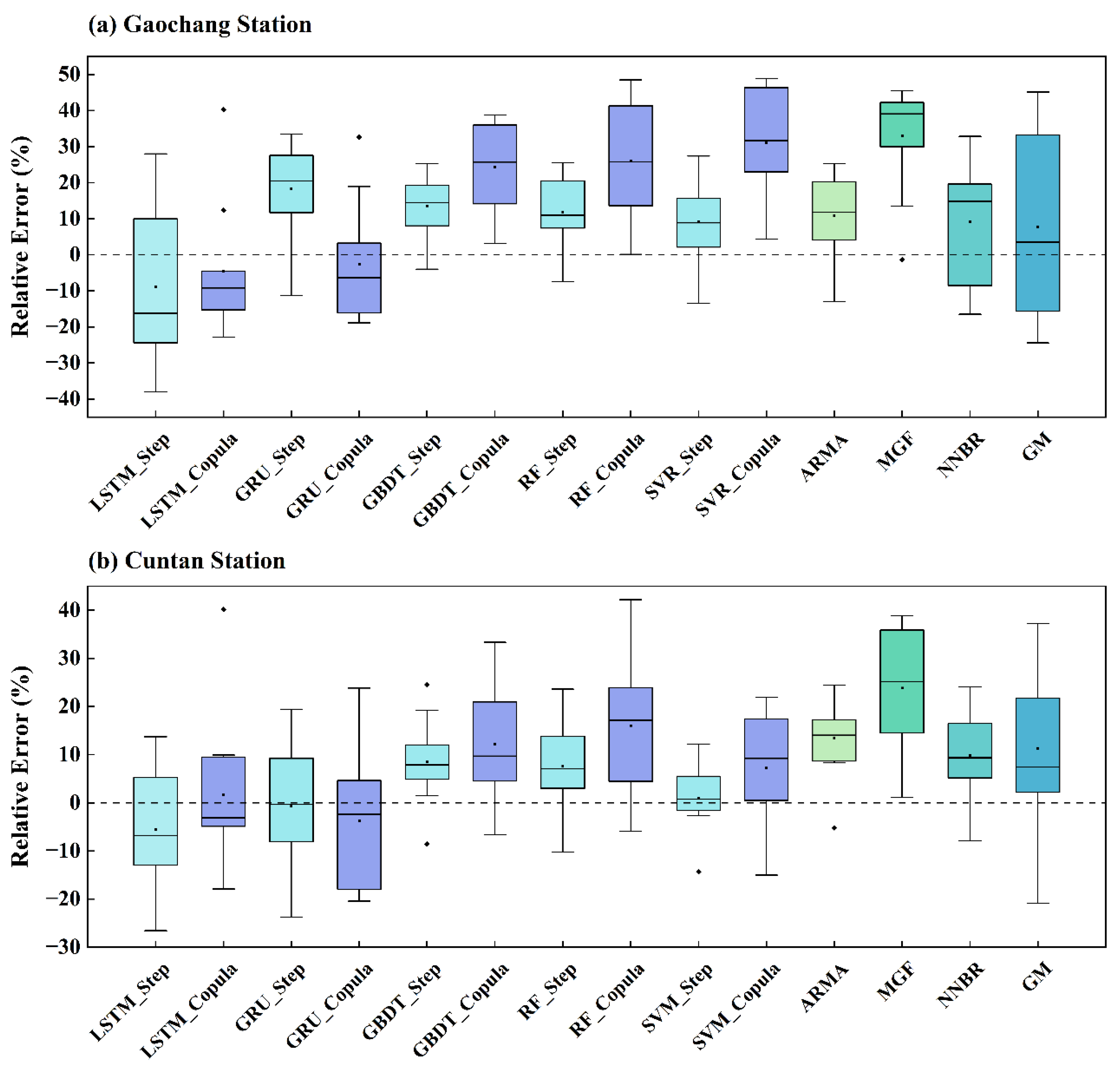
The predictions on the low flows were better than peak flows (Figures S3 and S4). For the Gaochang Station, generally, all ML models and univariate models tended to underestimate the low flows except the year 2010 to an average relative error of 14.49% (Figure 10). The distributions of relative error on annual peak flow prediction were denser than on annual low flows in the testing stage, especially LSTM_Copula model, GBDT_Step model, and RF_Step model. Besides, NNBR and GM did not show stable performance in predicting peak and low flows. For the Cuntan Station, the prediction performances on the low flows were better than the Gaochang Station, given that the streamflow is higher at the Cuntan Station. The ML models’ prediction results were close to the observation with an average relative error of 5.76%, and the distributions of ML models were denser than traditional statistical models. While the univariate models had a worse performance with an average relative error of 14.58%, MGF and GM models did not show good performance (Figure 11), indicating that the complex physical mechanism underlying extreme floods could not be captured by simple univariate models.

4. Discussion

Considering the effects of different variables and lag periods on runoff, we applied five common ML models with the traditional stepwise regression method and the copula entropy method to select the optimal variables and predict monthly streamflow for the Gaochang Station and the Cuntan Station. We also applied four univariate models as benchmarks to investigate the role of multi-variable input in monthly streamflow prediction.
The results revealed that input variables of different time lag influenced the prediction performance of runoff. Interestingly, the stepwise regression method selected more global circulation variables while the copula entropy method tended to select more ground meteorological variables. At the Gaochang Station, the variables impacting the runoff process include the northern hemisphere polar vortex central intensity Index with a lag of one month, the North American subtropical high area index with a lag of twelve months, the Tibet Plateau region 1 Index with a lag of one month, the Asia polar vortex area index with a lag of one month, the Indian Ocean warm pool strength index with a lag of nine months, suggesting that the streamflow processes in the UYRB are not only closely linked geographically to the Tibetan Plateau with pre-summer thawing of frozen soil [62,63,64,65], but also remotely influenced by the atmospheric circulation in the northern hemisphere, especially the East Asian monsoon circulation system, and the warm Indian Ocean condition and tropical SST anomalies [66,67,68,69], which can be found in the selected variables of the Cuntan Station as well.
Generally, the ML models outperform the univariate models in both the training and the testing stages. For instance, the LSTM_Copula model makes average improvements of 12.25, 8.71, 10.06, and 1.12% in the MAPE, RMSE, NSE, and R values than other ML models for the Gaochang Station and 6.59, 2.89, 5.19, and 0.66% for the Cuntan Station. In addition, the ML models outperform the univariate models on the annual low flows with much lower relative errors of 5.76 and 14.58% for the Gaochang Station and the Cuntan Station. However, the performance of ML and univariate models did not look distinct when predicting the annual peak flow, suggesting the difficulty of extreme runoff prediction. The comparative analysis above substantiates the vital part of meteorological variables input for data-driven models and confirms the superiority of the nonlinear and self-learning ML models.
The optimal models for monthly streamflow prediction differed between the two stations, which explains the complexity and difficulty of medium to long-term runoff prediction. However, some models outperformed others to a certain degree, and the comparison results illustrated the superiority of the copula entropy method and LSTM model. For the Gaochang Station, the LSTM_Copula model outperformed other models with better values of evaluation metrics and a more steady and robust effect in different months with 17.624% of MAPE, 691.492 m3/s of RMSE, 0.783 of NSE, and 0.937 of R in the testing stage, and the LSTM_Copula model obtained the best weighted average score of 0.078, which was similar to the previous research [70] in the Gaochang Station with ANN, ELM, and SVM models. Compared with the LSTM_Step, the LSTM_Copula improved the MAPE, RMSE, NSE, and R values by about 3.33, 5.19, 1.68, and 1.47% in the testing stage, respectively. Besides, it increased 20.48, 10.65, 11.49, and 3.25% in the MAPE, RMSE, NSE, and R values in the testing stage in comparison with the GBDT_Copula model. For the Cuntan Station, LSTM_Copula and RF_Copula models performed relatively better in general with 14.441~16.734% of MAPE, 2616.354~2782.648 m3/s of RMSE, 0.835~0.811 of NSE, and 0.960~0.962 of R in the testing stage, which is better in the MAPE and R values than the previous study [71] on the Cuntan Station.
Furthermore, some aspects limit the prediction accuracy and stability in this study. On the one hand, the ML models can theoretically reach the approximate solution, while the conventional gradient-based training technique tends to be stuck in the local minimum [72,73,74,75]. On the other hand, the calibration of hyperparameters greatly influences the forecasting models’ results. Furthermore, the computational cost of the ML models is longer than traditional statistical models since the models’ structure is more complex and the optimal parameter searching is time-consuming, which took 450~600 s for LSTM and GRU modeling, 120~200 s for the GBDT, RF, and SVR modeling, and 30~70 s for traditional statistical modeling in personal computers with 8 CPU and dual thread in our study. Besides, influenced by multiple variables in both the physical world and human society [76,77], the runoff process presents knotty dynamic characteristics, making it more challenging to predict. Accordingly, in some cases, a single model and limited input variables may not be able to make satisfactory predictions. Multiple-model coupling is inevitable in the future, and more work is needed to employ more input variables by novel algorithms [78,79,80] and to investigate the interpretability of the chosen variables based on the developed knowledge.

5. Conclusions

The stepwise regression and copula entropy methods were applied in five ML models for monthly streamflow prediction for the Gaochang Station and Cuntan Station in the UYRB, including the LSTM_Step, LSTM_Copula, GRU_Step, GRU_Copula, GBDT_Step, GBDT_Copula, RF_Step, RF_Copula, SVR_Step, and SVR_Copula. The results indicate that the LSTM_Copula model outperformed other models in predicting monthly runoff at the Gaochang Station and the Cuntan Station, whereas the GRU_Step and RF_Copula models also showed satisfactory performances. Besides, LSTM and GRU models tended to underestimate the peak flows while GBDT, RF, and SVR tended to overestimate them. This means that the accuracy of peak flow forecasting still needs improvement owing to the few extreme flood samples available for learning. In addition, compared with four univariate time series models (i.e., ARMA, MGF, NNBR, and GM), the ML models with multi-variables input generally presented better forecasting accuracy. In conclusion, we demonstrate that the proposed ML methods are potentially effective tools for monthly streamflow prediction, selecting appropriate input variables and time lags simultaneously.

Supplementary Materials

The following supporting information can be downloaded at: https://www.mdpi.com/article/10.3390/su141811149/s1, Figure S1: Observed runoff and simulated monthly runoff by univariate models for the Gaochang Station in the testing stage; Figure S2: Observed runoff and simulated monthly runoff by univariate models for the Cuntan Station in the testing stage; Figure S3: Annual peak flows of various models for the Gaochang Station and Cuntan Station in the testing stage; Figure S4: Annual low flows of various models for the Gaochang Station and Cuntan Station in the testing stage; Figure S5: The decision tree visualizing plot in the RF_Step model at Cuntan Station. Table S1: The candidate predictive variables for runoff forecasting models; Table S2: Statistical metrics of 1-month-ahead runoff forecasting results of ML models for the Gaochang Station and Cuntan Station; Table S3: Statistical metrics of 1-month-ahead runoff forecasting results of univariate models for the Gaochang Station and Cuntan Station.

Author Contributions

Conceptualization, X.L. and L.Z.; methodology, X.L. and S.Z.; software, X.L. and L.L.; formal analysis, X.L. and Z.T. (Zhengyang Tang); resources, S.Z.; writing—original draft preparation, X.L.; writing—review and editing, L.Z., S.Z., Q.Z., Z.T. (Zhenyu Tang) and X.H.; All authors have read and agreed to the published version of the manuscript.

Funding

This work was supported by the Hubei Key Laboratory of Intelligent Yangtze and Hydroelectric Science Foundation (Grant Number: ZH20020001). We also acknowledge support by the National Key Research and Development Program of China (Grant Number: 2017YFA0603704), the Major projects of the National Natural Science Foundation of China (Grant Number: 41890824), the Excellent Young Scientists Fund, the Strategic Priority Research Program of the Chinese Academy of Sciences (Grant Number: XDA23040500), and the Youth Innovation Promotion Association, CAS (Grant Number: 2021385).

Institutional Review Board Statement

Not applicable.

Informed Consent Statement

Not applicable.

Data Availability Statement

The data that support the findings of this study were derived from the following resources available in the public domain: monthly streamflow, https://data.cma.cn/ (accessed on 20 June 2022); monthly global circulation indexes, http://cmdp.ncc-cma.net (accessed on 20 June 2022); air pressure, average temperature, maximum temperature, minimum temperature, relative humidity, wind speed and daylight hours, https://data.cma.cn/ (accessed on 20 June 2022).

Acknowledgments

We thank the anonymous reviewers for their constructive feedback.

Conflicts of Interest

The authors declare no conflict of interest.

References

  1. Arora, A.; Arabameri, A.; Pandey, M.; Siddiqui, M.A.; Shukla, U.K.; Dieu Tien, B.; Mishra, V.N.; Bhardwaj, A. Optimization of state-of-the-art fuzzy-metaheuristic ANFIS-based machine learning models for flood susceptibility prediction mapping in the Middle Ganga Plain, India. Sci. Total Environ. 2021, 750, 141565. [Google Scholar] [CrossRef] [PubMed]
  2. Tabari, H. Extreme value analysis dilemma for climate change impact assessment on global flood and extreme precipitation. J. Hydrol. 2021, 593, 16. [Google Scholar] [CrossRef]
  3. Mosavi, A.; Ozturk, P.; Chau, K.-w. Flood Prediction Using Machine Learning Models: Literature Review. Water 2018, 10, 1536. [Google Scholar] [CrossRef]
  4. Lu, P.Y.; Lin, K.R.; Xu, C.Y.; Lan, T.; Liu, Z.Y.; He, Y.H. An integrated framework of input determination for ensemble forecasts of monthly estuarine saltwater intrusion. J. Hydrol. 2021, 598, 126225. [Google Scholar] [CrossRef]
  5. Feng, Z.-k.; Niu, W.-j.; Tang, Z.-y.; Jiang, Z.-q.; Xu, Y.; Liu, Y.; Zhang, H.-r. Monthly runoff time series prediction by variational mode decomposition and support vector machine based on quantum-behaved particle swarm optimization. J. Hydrol. 2020, 583, 124627. [Google Scholar] [CrossRef]
  6. Samantaray, S.; Das, S.S.; Sahoo, A.; Satapathy, D.P. Monthly runoff prediction at Baitarani river basin by support vector machine based on Salp swarm algorithm. Ain Shams Eng. J. 2022, 13, 101732. [Google Scholar] [CrossRef]
  7. Deb, P.; Kiem, A.S.; Willgoose, G. Mechanisms influencing non-stationarity in rainfall-runoff relationships in southeast Australia. J. Hydrol. 2019, 571, 749–764. [Google Scholar] [CrossRef]
  8. Xu, W.; Chen, J.; Zhang, X.J. Scale Effects of the Monthly Streamflow Prediction Using a State-of-the-art Deep Learning Model. Water Resour. Manag. 2022, 36, 3069–3625. [Google Scholar] [CrossRef]
  9. Zhang, F.; Kang, Y.; Cheng, X.; Chen, P.; Song, S. A Hybrid Model Integrating Elman Neural Network with Variational Mode Decomposition and Box–Cox Transformation for Monthly Runoff Time Series Prediction. Water Resour. Manag. 2022, 36, 3673–3697. [Google Scholar] [CrossRef]
  10. Ren, Y.; Zeng, S.; Liu, J.; Tang, Z.; Hua, X.; Li, Z.; Song, J.; Xia, J. Mid- to Long-Term Runoff Prediction Based on Deep Learning at Different Time Scales in the Upper Yangtze River Basin. Water 2022, 14, 1692. [Google Scholar] [CrossRef]
  11. Ai, P.; Song, Y.; Xiong, C.; Chen, B.; Yue, Z. A novel medium- and long-term runoff combined forecasting model based on different lag periods. J. Hydroinform. 2022, 24, 367–387. [Google Scholar] [CrossRef]
  12. Yaseen, Z.M.; Sulaiman, S.O.; Deo, R.C.; Chau, K.W. An enhanced extreme learning machine model for river flow forecasting: State-of-the-art, practical applications in water resource engineering area and future research direction. J. Hydrol. 2019, 569, 387–408. [Google Scholar] [CrossRef]
  13. Moosavi, V.; Gheisoori Fard, Z.; Vafakhah, M. Which one is more important in daily runoff forecasting using data driven models: Input data, model type, preprocessing or data length? J. Hydrol. 2022, 606, 127429. [Google Scholar] [CrossRef]
  14. Lall, U.; Sharma, A. A nearest neighbor bootstrap for resampling hydrologic time series. Water Resour. Res. 1996, 32, 679–693. [Google Scholar] [CrossRef]
  15. Mao, M.; Chirwa, E.C. Application of grey model GM (1, 1) to vehicle fatality risk estimation. Technol. Forecast. Soc. Chang. 2006, 73, 588–605. [Google Scholar] [CrossRef]
  16. McLeod, A.I.; Li, W.K. Diagnostic checking ARMA time series models using squared-residual autocorrelations. J. Time Ser. Anal. 1983, 4, 269–273. [Google Scholar] [CrossRef]
  17. Slay, J.C.; Solomon, J. A mean generating function. Two-Year Coll. Math. J. 1981, 12, 27–29. [Google Scholar] [CrossRef]
  18. Somu, N.; MR, G.R.; Ramamritham, K. A hybrid model for building energy consumption forecasting using long short term memory networks. Appl. Energy 2020, 261, 114131. [Google Scholar] [CrossRef]
  19. Chen, X.; Parajka, J.; Széles, B.; Strauss, P.; Blöschl, G. Controls on event runoff coefficients and recession coefficients for different runoff generation mechanisms identified by three regression methods. J. Hydrol. Hydromech. 2020, 68, 155–169. [Google Scholar] [CrossRef]
  20. Bojang, P.O.; Yang, T.-C.; Pham, Q.B.; Yu, P.-S. Linking Singular Spectrum Analysis and Machine Learning for Monthly Rainfall Forecasting. Appl. Sci. 2020, 10, 3224. [Google Scholar] [CrossRef]
  21. Niu, W.-j.; Feng, Z.-k.; Xu, Y.-s.; Feng, B.-f.; Min, Y.-w. Improving Prediction Accuracy of Hydrologic Time Series by Least-Squares Support Vector Machine Using Decomposition Reconstruction and Swarm Intelligence. J. Hydrol. Eng. 2021, 26, 04021030. [Google Scholar] [CrossRef]
  22. Abbasi, M.; Farokhnia, A.; Bahreinimotlagh, M.; Roozbahani, R. A hybrid of Random Forest and Deep Auto-Encoder with support vector regression methods for accuracy improvement and uncertainty reduction of long-term streamflow prediction. J. Hydrol. 2021, 597, 125717. [Google Scholar] [CrossRef]
  23. Cheng, Q.P.; Zuo, X.A.; Zhong, F.L.; Gao, L.; Xiao, S.C. Runoff variation characteristics, association with large-scale circulation and dominant causes in the Heihe River Basin, Northwest China. Sci. Total Environ. 2019, 688, 361–379. [Google Scholar] [CrossRef]
  24. Zhang, Y.; Wang, M.L.; Chen, J.; Zhong, P.A.; Wu, X.F.; Wu, S.Q. Multiscale attribution analysis for assessing effects of changing environment on runoff: Case study of the Upstream Yangtze River in China. J. Water Clim. Chang. 2021, 12, 627–646. [Google Scholar] [CrossRef]
  25. Tao, L.Z.; He, X.G.; Li, J.J.; Yang, D. A multiscale long short-term memory model with attention mechanism for improving monthly precipitation prediction. J. Hydrol. 2021, 602, 126815. [Google Scholar] [CrossRef]
  26. May, R.J.; Maier, H.R.; Dandy, G.C.; Fernando, T. Non-linear variable selection for artificial neural networks using partial mutual information. Environ. Model. Softw. 2008, 23, 1312–1326. [Google Scholar] [CrossRef]
  27. Yang, X.; Li, Y.P.; Liu, Y.R.; Gao, P.P. A MCMC-based maximum entropy copula method for bivariate drought risk analysis of the Amu Darya River Basin. J. Hydrol. 2020, 590, 125502. [Google Scholar] [CrossRef]
  28. Ma, J.; Sun, Z. Mutual Information Is Copula Entropy. Tsinghua Sci. Technol. 2011, 16, 51–54. [Google Scholar] [CrossRef]
  29. Singh, V.P.; Zhang, L. Copula-entropy theory for multivariate stochastic modeling in water engineering. Geosci. Lett. 2018, 5, 1–17. [Google Scholar] [CrossRef]
  30. Hao, Z.; Singh, V.P. Integrating Entropy and Copula Theories for Hydrologic Modeling and Analysis. Entropy 2015, 17, 2253–2280. [Google Scholar] [CrossRef] [Green Version]
  31. AghaKouchak, A. Entropy-Copula in Hydrology and Climatology. J. Hydrometeorol. 2014, 15, 2176–2189. [Google Scholar] [CrossRef]
  32. Qin, P.; Xu, H.; Liu, M.; Du, L.; Xiao, C.; Liu, L.; Tarroja, B. Climate change impacts on Three Gorges Reservoir impoundment and hydropower generation. J. Hydrol. 2020, 580, 123922. [Google Scholar] [CrossRef]
  33. Niu, X. Key Technologies of the Hydraulic Structures of the Three Gorges Project. Engineering 2016, 2, 340–349. [Google Scholar] [CrossRef]
  34. Xiong, L.H.; Guo, S.L. Trend test and change-point detection for the annual discharge series of the Yangtze River at the Yichang hydrological station. Hydrol. Sci. J.-J. Des. Sci. Hydrol. 2004, 49, 99–112. [Google Scholar] [CrossRef]
  35. Zhang, Y.; Zhong, P.-a.; Wang, M.; Xu, B.; Chen, J. Changes identification of the Three Gorges reservoir inflow and the driving factors quantification. Quat. Int. 2018, 475, 28–41. [Google Scholar] [CrossRef]
  36. Liu, Y.; Hou, G.; Huang, F.; Qin, H.; Wang, B.; Yi, L. Directed graph deep neural network for multi-step daily streamflow forecasting. J. Hydrol. 2022, 607, 127515. [Google Scholar] [CrossRef]
  37. Xu, J. Trends in suspended sediment grain size in the upper Yangtze River and its tributaries, as influenced by human activities. Hydrol. Sci. J.-J. Des. Sci. Hydrol. 2007, 52, 777–792. [Google Scholar] [CrossRef]
  38. Zhang, X.; Zheng, Z.; Wang, K. Prediction of runoff in the upper Yangtze River based on CEEMDAN-NAR model. Water Supply 2021, 21, 3307–3318. [Google Scholar] [CrossRef]
  39. Yang, X.L.; Yu, X.H.; Wang, Y.Q.; Liu, Y.; Zhang, M.R.; Ren, L.L.; Yuan, F.; Jiang, S.H. Estimating the response of hydrological regimes to future projections of precipitation and temperature over the upper Yangtze River. Atmos. Res. 2019, 230, 104627. [Google Scholar] [CrossRef]
  40. Luo, K.S.; Li, Y.Z. Assessing rainwater harvesting potential in a humid and semi-humid region based on a hydrological model. J. Hydrol. Reg. Stud. 2021, 37, 100912. [Google Scholar] [CrossRef]
  41. Chen, J.; Finlayson, B.L.; Wei, T.Y.; Sun, Q.L.; Webber, M.; Li, M.T.; Chen, Z.Y. Changes in monthly flows in the Yangtze River, China—With special reference to the Three Gorges Dam. J. Hydrol. 2016, 536, 293–301. [Google Scholar] [CrossRef]
  42. Libiseller, C.; Grimvall, A. Performance of partial Mann-Kendall tests for trend detection in the presence of covariates. Environmetrics 2002, 13, 71–84. [Google Scholar] [CrossRef]
  43. Sen, P.K. Estimates of the regression coefficient based on Kendall’s tau. J. Am. Stat. Assoc. 1968, 63, 1379–1389. [Google Scholar] [CrossRef]
  44. Pettitt, A.N. A non-parametric approach to the change-point problem. J. R. Stat. Soc. Ser. C Appl. Stat. 1979, 28, 126–135. [Google Scholar] [CrossRef]
  45. Aljoda, A.; Jain, S. Uncertainties and risks in reservoir operations under changing hydroclimatic conditions. J. Water Clim. Chang. 2021, 12, 1708–1723. [Google Scholar] [CrossRef]
  46. Erdem, O.; Ceyhan, E.; Varli, Y. A new correlation coefficient for bivariate time-series data. Phys. A Stat. Mech. Its Appl. 2014, 414, 274–284. [Google Scholar] [CrossRef]
  47. Sharma, A.; Luk, K.; Cordery, I.; Lall, U. Seasonal to interannual rainfall probabilistic forecasts for improved water supply management: Part 2—Predictor identification of quarterly rainfall using ocean-atmosphere information. J. Hydrol. 2000, 239, 240–248. [Google Scholar] [CrossRef]
  48. Gao, S.; Huang, Y.; Zhang, S.; Han, J.; Wang, G.; Zhang, M.; Lin, Q. Short-term runoff prediction with GRU and LSTM networks without requiring time step optimization during sample generation. J. Hydrol. 2020, 589, 125188. [Google Scholar] [CrossRef]
  49. Yuan, X.; Chen, C.; Lei, X.; Yuan, Y.; Muhammad Adnan, R. Monthly runoff forecasting based on LSTM–ALO model. Stoch. Environ. Res. Risk Assess. 2018, 32, 2199–2212. [Google Scholar] [CrossRef]
  50. Fischer, T.; Krauss, C. Deep learning with long short-term memory networks for financial market predictions. Eur. J. Oper. Res. 2018, 270, 654–669. [Google Scholar] [CrossRef] [Green Version]
  51. Kratzert, F.; Klotz, D.; Brenner, C.; Schulz, K.; Herrnegger, M. Rainfall–runoff modelling using Long Short-Term Memory (LSTM) networks. Hydrol. Earth Syst. Sci. 2018, 22, 6005–6022. [Google Scholar] [CrossRef]
  52. Wang, Q.Y.; Zheng, Y.X.; Yue, Q.M.; Liu, Y.; Yu, J.S. Regional characteristics’ impact on the performances of the gated recurrent unit on streamflow forecasting. Water Supply 2022, 22, 4142–4158. [Google Scholar] [CrossRef]
  53. Wang, Q.Y.; Liu, Y.; Yue, Q.M.; Zheng, Y.X.; Yao, X.L.; Yu, J.S. Impact of Input Filtering and Architecture Selection Strategies on GRU Runoff Forecasting: A Case Study in the Wei River Basin, Shaanxi, China. Water 2020, 12, 3532. [Google Scholar] [CrossRef]
  54. Breiman, L. Random forests. Mach. Learn. 2001, 45, 5–32. [Google Scholar] [CrossRef]
  55. Wu, Z.; Zhou, Y.; Wang, H.; Jiang, Z. Depth prediction of urban flood under different rainfall return periods based on deep learning and data warehouse. Sci. Total Environ. 2020, 716, 137077. [Google Scholar] [CrossRef]
  56. Yang, T.T.; Asanjan, A.A.; Welles, E.; Gao, X.G.; Sorooshian, S.; Liu, X.M. Developing reservoir monthly inflow forecasts using artificial intelligence and climate phenomenon information. Water Resour. Res. 2017, 53, 2786–2812. [Google Scholar] [CrossRef]
  57. Vapnik, V. The Nature of Statistical Learning Theory; Springer Science & Business Media: Berlin/Heidelberg, Germany, 1999. [Google Scholar]
  58. Cortes, C.; Vapnik, V. Support-vector networks. Mach. Learn. 1995, 20, 273–297. [Google Scholar] [CrossRef]
  59. Parisouj, P.; Mohebzadeh, H.; Lee, T. Employing Machine Learning Algorithms for Streamflow Prediction: A Case Study of Four River Basins with Different Climatic Zones in the United States. Water Resour. Manag. 2020, 34, 4113–4131. [Google Scholar] [CrossRef]
  60. Arnold, J.G.; Moriasi, D.N.; Gassman, P.W.; Abbaspour, K.C.; White, M.J.; Srinivasan, R.; Santhi, C.; Harmel, R.; Van Griensven, A.; Van Liew, M.W. SWAT: Model use, calibration, and validation. Trans. ASABE 2012, 55, 1491–1508. [Google Scholar] [CrossRef]
  61. Wang, W.-c.; Chau, K.-w.; Qiu, L.; Chen, Y.-b. Improving forecasting accuracy of medium and long-term runoff using artificial neural network based on EEMD decomposition. Environ. Res. 2015, 139, 46–54. [Google Scholar] [CrossRef]
  62. Li, Y.H.; Wang, T.H.; Yang, D.W.; Tang, L.H.; Yang, K.; Liu, Z.W. Linkage between anomalies of pre-summer thawing of frozen soil over the Tibetan Plateau and summer precipitation in East Asia. Environ. Res. Lett. 2021, 16, 114030. [Google Scholar] [CrossRef]
  63. Lei, Y.H.; Shi, J.C.; Xiong, C.A.; Ji, D. Tracking the Atmospheric-Terrestrial Water Cycle over the Tibetan Plateau Based on ERA5 and GRACE. J. Clim. 2021, 34, 6459–6471. [Google Scholar] [CrossRef]
  64. Ma, T.T.; Wu, G.X.; Liu, Y.M.; Mao, J.Y. Abnormal warm sea-surface temperature in the Indian Ocean, active potential vorticity over the Tibetan Plateau, and severe flooding along the Yangtze River in summer 2020. Q. J. R. Meteorol. Soc. 2022, 148, 1001–1019. [Google Scholar] [CrossRef]
  65. Wang, Y.; Ye, A.; Peng, D.; Miao, C.; Di, Z.; Gong, W. Spatiotemporal variations in water conservation function of the Tibetan Plateau under climate change based on InVEST model. J. Hydrol. Reg. Stud. 2022, 41, 101064. [Google Scholar] [CrossRef]
  66. Ding, Y.H.; Liu, Y.Y.; Hu, Z.Z. The Record-breaking Meiyu in 2020 and Associated Atmospheric Circulation and Tropical SST Anomalies. Adv. Atmos. Sci. 2021, 38, 1980–1993. [Google Scholar] [CrossRef]
  67. Wei, W.; Zhang, R.H.; Yang, S.; Li, W.H.; Wen, M. Quasi-Biweekly Oscillation of the South Asian High and Its Role in Connecting the Indian and East Asian Summer Rainfalls. Geophys. Res. Lett. 2019, 46, 14742–14750. [Google Scholar] [CrossRef]
  68. Zhou, Z.Q.; Xie, S.P.; Zhang, R.H. Historic Yangtze flooding of 2020 tied to extreme Indian Ocean conditions. Proc. Natl. Acad. Sci. USA 2021, 118, e2022255118. [Google Scholar] [CrossRef]
  69. Takaya, Y.; Ishikawa, I.; Kobayashi, C.; Endo, H.; Ose, T. Enhanced Meiyu-Baiu Rainfall in Early Summer 2020: Aftermath of the 2019 Super IOD Event. Geophys. Res. Lett. 2020, 47, e2020GL090671. [Google Scholar] [CrossRef]
  70. Feng, Z.-k.; Niu, W.-j. Hybrid artificial neural network and cooperation search algorithm for nonlinear river flow time series forecasting in humid and semi-humid regions. Knowl. Based Syst. 2021, 211, 106580. [Google Scholar] [CrossRef]
  71. Niu, W.-j.; Feng, Z.-k. Evaluating the performances of several artificial intelligence methods in forecasting daily streamflow time series for sustainable water resources management. Sustain. Cities Soc. 2021, 64, 102562. [Google Scholar] [CrossRef]
  72. Pham, B.T.; Le, L.M.; Le, T.T.; Bui, K.T.T.; Le, V.M.; Ly, H.B.; Prakash, I. Development of advanced artificial intelligence models for daily rainfall prediction. Atmos. Res. 2020, 237, 15. [Google Scholar] [CrossRef]
  73. Tiyasha; Tung, T.M.; Yaseen, Z.M. A survey on river water quality modelling using artificial intelligence models: 2000–2020. J. Hydrol. 2020, 585, 62. [Google Scholar]
  74. Wang, Z.Y.; Srinivasan, R.S. A review of artificial intelligence based building energy use prediction: Contrasting the capabilities of single and ensemble prediction models. Renew. Sust. Energ. Rev. 2017, 75, 796–808. [Google Scholar] [CrossRef]
  75. Meng, E.H.; Huang, S.Z.; Huang, Q.; Fang, W.; Wu, L.Z.; Wang, L. A robust method for non-stationary streamflow prediction based on improved EMD-SVM model. J. Hydrol. 2019, 568, 462–478. [Google Scholar] [CrossRef]
  76. Yoosefdoost, I.; Khashei-Siuki, A.; Tabari, H.; Mohammadrezapour, O. Runoff Simulation Under Future Climate Change Conditions: Performance Comparison of Data-Mining Algorithms and Conceptual Models. Water Resour. Manag. 2022, 36, 1191–1215. [Google Scholar] [CrossRef]
  77. Demir, V. Enhancing monthly lake levels forecasting using heuristic regression techniques with periodicity data component: Application of Lake Michigan. Theor. Appl. Climatol. 2022, 143, 915–929. [Google Scholar] [CrossRef]
  78. Rathnayake, N.; Rathnayake, U.; Tuan Linh, D.; Hoshino, Y. A Cascaded Adaptive Network-Based Fuzzy Inference System for Hydropower Forecasting. Sensors 2022, 22, 2905. [Google Scholar] [CrossRef]
  79. Rathnayake, N.; Dang, T.L.; Hoshino, Y. A Novel Optimization Algorithm: Cascaded Adaptive Neuro-Fuzzy Inference System. Int. J. Fuzzy Syst. 2021, 23, 1955–1971. [Google Scholar] [CrossRef]
  80. Chaudhari, S.; Mithal, V.; Polatkan, G.; Ramanath, R. An Attentive Survey of Attention Models. Acm Trans. Intell. Syst. Technol. 2021, 12, 1–32. [Google Scholar] [CrossRef]
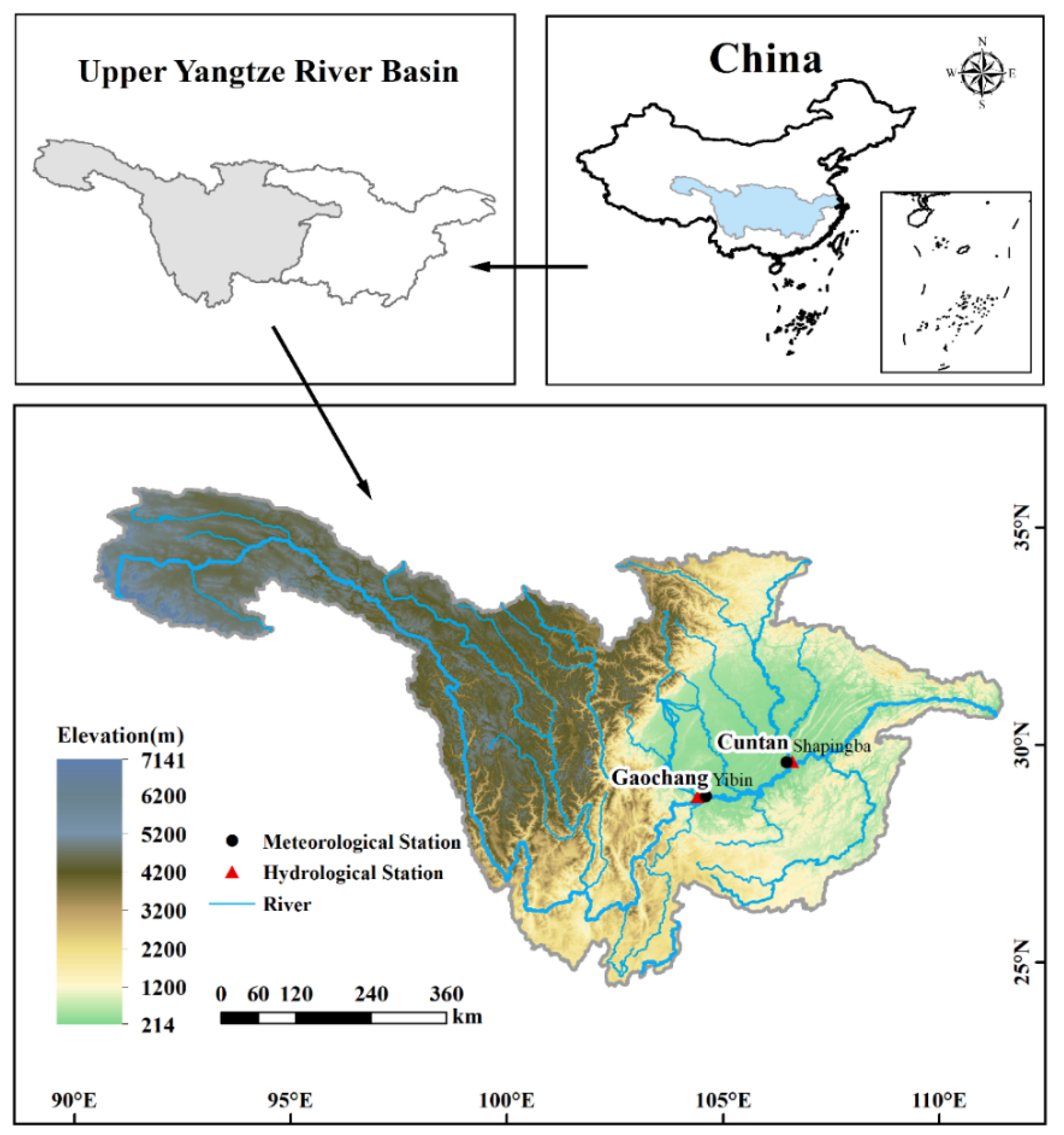
Figure 1. The Upper Yangtze River Basin (UYRB). This study is focused on two hydrological stations—Gaochang and Cuntan, and two meteorological stations nearby—Yibin and Shapingba.
Sustainability 14 11149 g001
Figure 2. (a) Runoff series and trend analysis of the Gaochang Station: the blue solid line is the runoff series and the red line shows the trend of the series. The contour of the wavelet coefficient is displayed in (c) and the wavelet variance is shown in (e). (b,d,f) represent the same information as (a,c,e), but for the Cuntan Station.
Sustainability 14 11149 g002
Figure 3. (a) The construction of a fundamental LSTM cell. (b) The construction of a fundamental GRU cell. In Figure 3a, W x i , W h i , W x f , W h f , W x o , W h o , W x C , and W h C are the network weights matrices. b i , b f , b o , and   b c are bias vectors. f t ,   i t , and o t are the activation value vectors of the forget gate, the input gate, and the output gate. Similarly, in Figure 3b, W x r , W h r , W x Z , W h Z are the network weights metrics, b r and   b Z are bias vectors.   r t and Z t are vectors for the update and reset gate activation values.
Sustainability 14 11149 g003
Figure 4. Flowchart of model development for predicting monthly runoff.
Sustainability 14 11149 g004
Figure 5. Variable selection results for the Gaochang Station (a) and Cuntan Station (b) by the copula entropy method. CE denotes the copula entropy, and Z represents the Hampel distance after the Hample test. The greater the CE value or Z value, the more significant the effect of the corresponding variable.
Sustainability 14 11149 g005
Figure 6. (a) The parameter optimization process of hidden_size in the LSTM_Copula model at Gaochang Station. (b) The optimal result of epochs in the GRU_Step model at Cuntan Station. (c) The simplified decision tree visualizing plot in the RF_Step model at Cuntan Station. (d) The best cost (c) and gamma (g) in the SVR_Step and SVR_Copula model at Gaochang Station.
Sustainability 14 11149 g006
Figure 7. Comparison of simulated with observed monthly runoff in the testing stage by the machine learning models for the Gaochang Station.
Sustainability 14 11149 g007
Figure 8. Comparison of simulated with observed monthly runoff in the testing stage by the machine learning models for the Cuntan Station.
Sustainability 14 11149 g008
Figure 9. The weighted average scores of MAPE, RMSE, NSE, and R by machine learning models and univariate models at the Gaochang Station (a) and the Cuntan Station (b) in the testing stage. The pink pentagram denotes the best score.
Sustainability 14 11149 g009
Figure 10. Relative errors of annual peak flow prediction by machine learning models and univariate models at the Gaochang Station (a) and Cuntan Station (b) in the testing stage.
Sustainability 14 11149 g010
Figure 11. Relative errors of annual low flow prediction by machine learning models and univariate models at the Gaochang Station (a) and Cuntan Station (b) in the testing stage. The black rhombus denote the anomaly.
Sustainability 14 11149 g011
Table 1. Variables selected by stepwise regression and copula entropy for the Gaochang Station and Cuntan Station.
StationStepwise RegressionCopula Entropy
VariablesLag
(Month)
VariablesLag
(Month)
GaochangAverage Temperature7Maximum Temperature1
Runoff12East Asian Trough Intensity Index6
Northern Hemisphere Polar Vortex Central Intensity Index1Average Temperature7
Maximum Temperature6Daylight Hours2
North American Subtropical High Area Index12Maximum Temperature7
Runoff1Runoff6
Relative Humidity1Daylight Hours1
Tibet Plateau Region 1 Index5East Asian Trough Intensity Index12
Asia Polar Vortex Area Index1Average Temperature1
Indian Ocean Warm Pool Strength Index9Runoff12
CuntanMaximum Temperature7Maximum Temperature7
Runoff12Maximum Temperature1
Northern Hemisphere Polar Vortex Intensity Index2Average Temperature7
Runoff1East Asian Trough Intensity Index7
North American Subtropical High Intensity Index12Runoff6
Atlantic-European Polar Vortex Intensity Index7Average Temperature1
Daylight Hours12Runoff12
Asia Polar Vortex Intensity Index6East Asian Trough Intensity Index1
Eurasian Zonal Circulation Index9Daylight Hours8
Air Pressure3Daylight Hours2
Publisher’s Note: MDPI stays neutral with regard to jurisdictional claims in published maps and institutional affiliations.