A New Model Predictive Control Method for Buck-Boost Inverter-Based Photovoltaic Systems

Abstract

This study designed a system consisting of a photovoltaic system and a DC-DC boost converter with buck-boost inverter. A multi-error method, based on model predictive control (MPC), is presented for control of the buck-boost inverter. Incremental conductivity and predictive control methods have also been used to track the maximum power of the photovoltaic system. Due to the fact that inverters are in the category of systems with fast dynamics, in this method, by first determining the system state space and its discrete time model, a switching algorithm is proposed to reduce the larger error for the converter. By using this control method, in addition to reducing the total harmonic distortion (THD), the inverter voltage reaches the set reference value at a high speed. To evaluate the performance of the proposed method, the dynamic performance of the converter at the reference voltage given to the system was investigated. The results of system performance in SIMULINK environment were simulated and analyzed by MATLAB software. According to the simulation results, we can point out the advantage of this system in following the reference signal with high speed and accuracy.

1. Introduction

With the increase in population and the advancement of technology, the need for electricity has become one of the essential needs of society and the available power is not enough. The construction of fossil power plants is very expensive. Moreover, these power plants are very harmful to the environment due to the production of carbon dioxide. For these reasons, the use of renewable energy is increasing day by day. Photovoltaic systems, which use solar energy to generate electricity, are one of the most popular methods of generating power. The output power of these systems is DC, so in order to transfer this power to the distribution network, we need to use a DC to AC converter (inverter). There are different types of inverters. One of the best types is the single-stage inverter [1,2,3,4,5,6,7].

Given the important task of the inverter in photovoltaic systems, a system should be used to control it with a fast dynamic response and high flexibility. One of the best methods to be used for many applications is model predictive control (MPC). Predictive control first predicts the future behavior of the system on a limited time horizon. Then, at any time, future input signals are calculated by minimizing a target function under the state constraints and input on the line [8,9]. Finally, only the first calculated control member is applied to the actual system and the previous steps are repeated by measuring the new mode, output, and input variables. Therefore, the presence of a proper model of the actual system is a prerequisite for design control [10,11]. MPC control has been developed in the electrical control industry and has recently been introduced to the power field. This includes three-phase DC-AC and AC-DC systems as well as DC-DC converters [12,13].

The control algorithm used in the industry should have favorable capabilities, including ease of use and adjustment, which will actually be a criterion for expanding its industrial application. Although the use of a PID (proportional–integral–derivative) controller is common in the industry, industrial processes are a dynamic, wide range of different behaviors that limit the use of such a controller [14,15]. The advantage that the MPC method has over other converter control methods, such as sliding mode control, is that the closed-loop stability issue is addressed as well as predictive control of single-input single-output systems (SISO), and multi-input multi-output (MIMO) has continuous and discrete modes. MPC has significant advantages over existing integral methods. This controller, which has a cost function, can increase the accuracy and also reduce the total harmonic distortion (THD). By predicting the future of the system, this controller can prepare for possible changes and have a more appropriate response than other methods [16,17].

Various predictive control methods and algorithms have been proposed to control power converters, indicating that these methods have potentially many advantages over pulse-width modulation (PWM) controllers. It also shows that model predictive control (MPC) is a very good alternative to controlling power converters and drives [18,19,20]. One type of controller is continuous nonlinear model predictive control (CNMPC), which can be used to control the power exchanged in a PV system. One of the disadvantages of this controller is that due to its nonlinearity, it cannot completely eliminate the steady state error [21]. The concept of MPC can be used in a photovoltaic system for tracking maximum power point (MPPT). In [22], this is carried out for a Z-source inverter, with a grid-connected PV system. This method has a simple structure and high performance. An improved prediction control strategy of the battery storage inverter, which prevents a large prediction error in the battery storage inverter, is presented in [23]. In [24], with the aim of supplying AC load through a single DC-AC converter, a model predictive control method was performed in photovoltaic systems. Moreover, due to the importance of current source inverters, several studies have investigated the structure of current source inverters using predictive mode control [25,26]. In [27], a new basic structure for multilevel inverters is presented, which can be developed in two different ways, and by reducing the number of components in these converters, more levels of voltage are generated. In all the studied works, only one of the error parameters (capacitor voltage or inductor current) has been examined. This can affect the stability and speed of the system. Moreover, most of the previous analyses are applicable only to certain classes of nonlinear systems and are suitable for simple cases. In addition, some of the previous analyses are complex and require great computational effort, and this is not desirable.

In this paper, a new two-error control technique using MPC as a voltage controller for a single-stage DC-AC inverter is proposed. The main purpose of the controller is to regulate the output voltage to the given value, which can be more or less than the input voltage. In order to increase the speed and stability, two error parameters have been used for better control of the system. For this purpose, first, the system state space, then the discrete model of the converter time is obtained and the new predictive control algorithm for the converter is presented. To evaluate the performance of the proposed method, the dynamic performance of the converter under the given reference voltage conditions is investigated. The proposed design has high speed and accuracy in tracking the reference signal. Moreover, the design process is simple and fewer calculations are performed than in similar designs. The designed system is shown in Figure 1.

The main contributions of this paper are as follows:

• Design of a photovoltaic system
• Tracking the maximum power point with MPC
• Presenting a two-error and MAC hybrid control method to regulate the output voltage of the inverter

The rest of the paper is organized as follows: Section 2 discusses the designed panel. The maximum power point tracking algorithm, which is implemented on the photovoltaic system, is given in Section 3. The specifications of the proposed inverter are listed in Section 4. The MPC strategy implemented on the inverter is described in Section 5. Section 6 fully describes the system simulation results, and in Section 7, the conclusion is given.

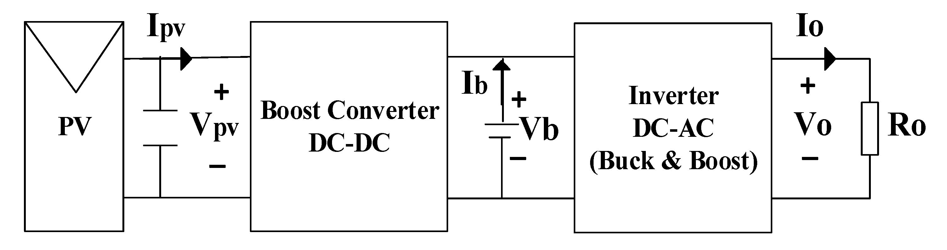
2. Designed Photovoltaic Panel

The designed panel (for radiation, 1000 W/m² and temperature of 25 °C) has a 3.8 A short circuit current and 21 V open circuit voltage. The optimum current and voltage are 3.57 A and 17.9 V, respectively. The maximum power of each simulated module using the optimal voltage and current is equal to 64 W. Additionally, for radiation of 700 W and temperature of 25 degrees Celsius, the optimum current and voltage for each module are 2.5 A and 17.5 V, respectively [28,29].

To produce 200 W of power using the designed module, we need four modules. It is necessary to close the two solar modules together in series and also in parallel with the other two modules. In this case, we form a photovoltaic system. If we series two modules, and parallel them with two other series modules, its power is obtained as follows:

$$\begin{array}{l}{\mathrm{V}}_{\mathrm{MPPT}}=2\times 17.9=35.8 \mathrm{V}\\ {\mathrm{I}}_{\mathrm{MPPT}}=2\times 3.57=7.15 \mathrm{A}\\ {\mathrm{P}}_{\mathrm{MPPT}}={\mathrm{V}}_{\mathrm{MPPT}}\times {\mathrm{I}}_{\mathrm{MPPT}}=256 \mathrm{W}\end{array}$$

(1)

The maximum current and voltage of the panel, assuming 700 W of radiation and a temperature of 25 °C, is obtained as Equation (2).

$$\begin{array}{l}{\mathrm{V}}_{\mathrm{MPPT}}=2\times 17.5=35 \mathrm{V}\\ {\mathrm{I}}_{\mathrm{MPPT}}=2\times 2.5=5 \mathrm{A}\\ {\mathrm{P}}_{\mathrm{MPPT}}={\mathrm{V}}_{\mathrm{MPPT}}\times {\mathrm{I}}_{\mathrm{MPPT}}=175 \mathrm{W}\end{array}$$

(2)

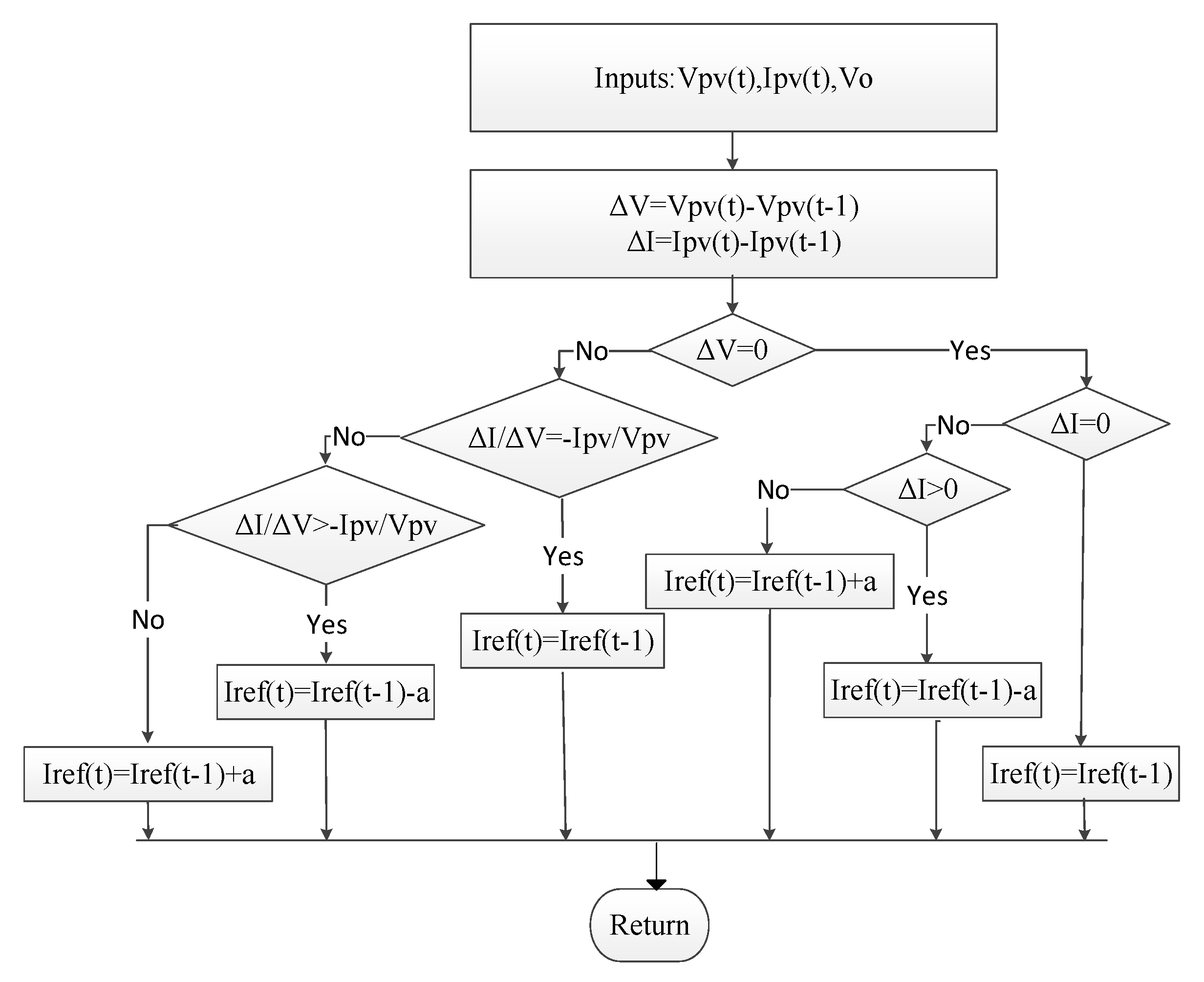
3. Maximum Power Point Tracking (MPPT)

Getting the maximum power from photovoltaic systems is important and essential in increasing the efficiency of these systems. Due to the uncertainty of the output power of photovoltaic systems, which depends on several factors such as radiation, temperature, and load size, these systems rarely operate at the maximum power point. Therefore, tracking the maximum power point plays an important role in increasing the efficiency of these systems. In this paper, to control the maximum power point, a control method consisting of three parts is used. First, the reference current is obtained using the incremental conductivity algorithm. Then, with the help of boost converter modeling and using the predictive control, the converter condition is predicted. Finally, using a cost function by reducing the reference current error relative to the predicted panel current, switching of the boost converter, so that the system operates at its maximum power point. Figure 2 shows the incremental conductivity algorithm used. The MPPT algorithm flowchart using the MPC method is shown in Figure 3. The parameters of the boost converter used in this paper are also shown in

Table 1. Boost Converter Parameters.

Parameter	Size
Inductance (L)	0.5 mH
Capacitor (C)	3000 µF
Sampling time (Ts)	10 µs

.

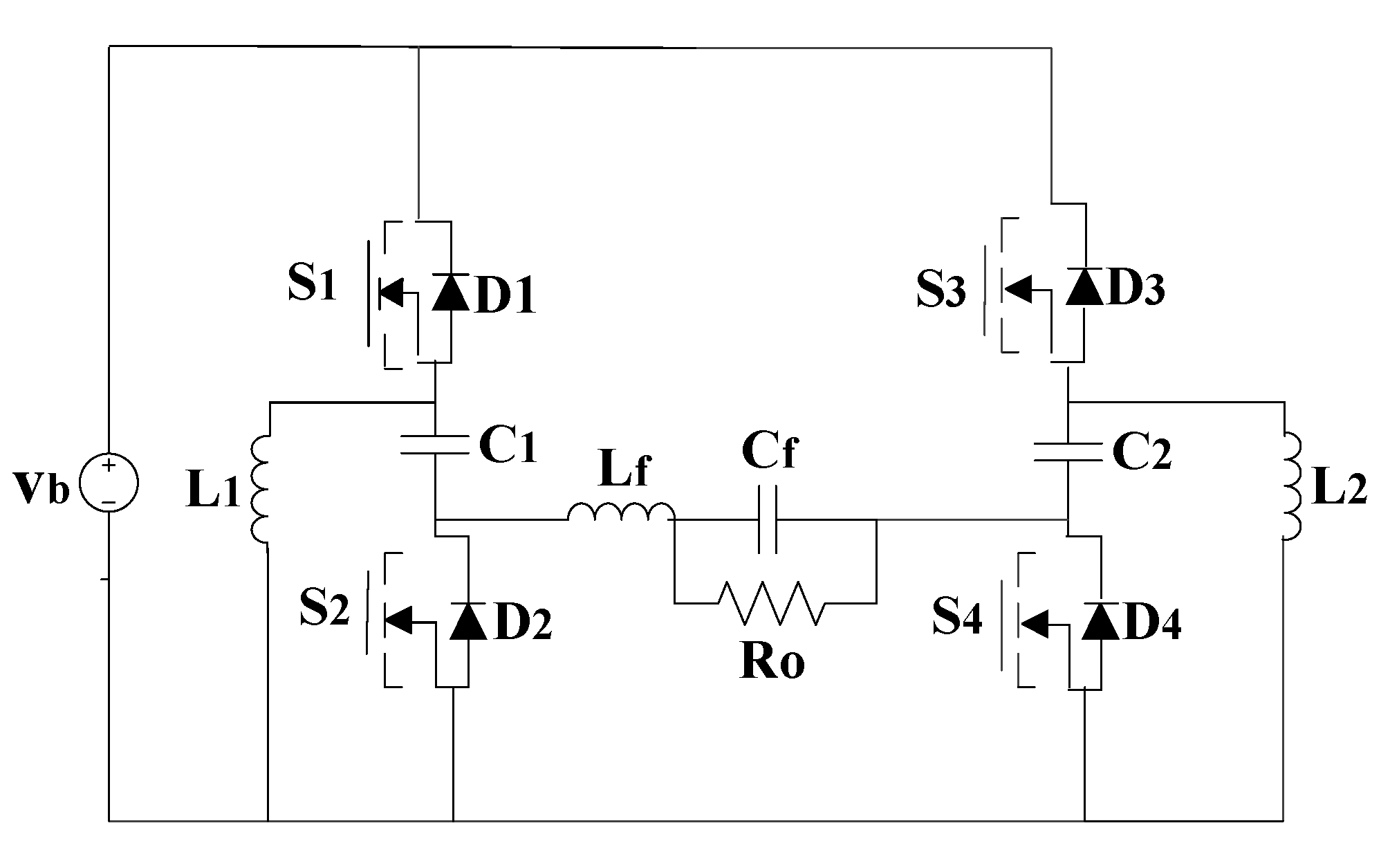
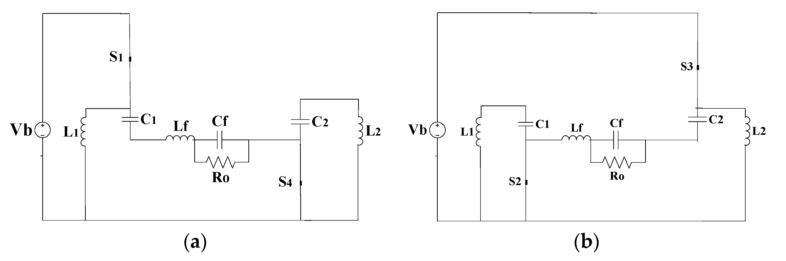
4. Single-Stage Inverter

As shown in Figure 4, the proposed single-stage inverter structure has a battery as the voltage source, a high frequency filter, load, and various switches.

In the proposed inverter, two switching models may occur. In the first case, switches 1 and 4 are on, and switches 3 and 2 are off. In the second case, the opposite happens, i.e., switches 2 and 3 are on, and switches 1 and 4 are off. In the first case, the inductor current L1 is increased, but inductor current L2 and capacitors voltage C1 and C2 are decreased. Equation (3) represents the converter state space. In this equation, A₁, A₂, B, and C are the matrices of the system, and y is the output of the system.

$$\begin{array}{l}\frac{dx(t)}{dt}=\left(A_1+A_{2}U(t)\right)x(t)+B{V}_s\\ y(t)=Cx(t)\end{array}$$

(3)

The state vector includes the currents of inductors L1, L2, and Lf and the voltages of capacitors C1, C2, and Cf are as follows:

$$x(t)={\left[i_{L1}(t) V_{C1}(t) i_{Lf}(t) V_{Cf}(t) V_{C2}(t) i_{L2}(t)\right]}^T$$

(4)

In the above equation, i and v represent the current and voltage of the inductors and capacitors mentioned in Figure 4. The output voltage (VO) is equal to the voltage passing through the Cf capacitor and the voltage across the load.

The following four matrices are inverter matrices which are defined as follows: U(t) can be considered as the status of switches and y(t) can be considered as the output of the system. When the switches are on, U(t) = 1, and in the case when the switches are turned off, U(t) = 0.

$$A_1=\left[\begin{array}{llllll}0& 0& 0& 0& 0& 0\\ 0& 0& 1/C_1& 0& 0& 0\\ 0& 1/L_f& 0& -1/L_f& 0& 0\\ 0& 0& 1/C_f& -1/R_o*C_f& 0& 0\\ 0& 0& 0& 0& 0& 1/C_2\\ 0& 0& 0& 0& -1/L_2& 0\end{array}\right]$$

(5)

$$A_2=\left[\begin{array}{llllll}0& -1/L_1& 0& 0& 0& 0\\ 1/C_1& 0& 0& 0& 0& 0\\ 0& 0& 0& -1/L_f& -1/L_f& 0\\ 0& 0& 1/C_f& -1/R_o*C_f& 0& 0\\ 0& 0& 1/C_2& 0& 0& 0\\ 0& 0& 0& 0& 0& 0\end{array}\right]$$

(6)

$$\begin{array}{l}{B}_1={\left[1/L_1 0 1/L_f 0 0 0\right]}^T\\ B_2={\left[0 0 -1/L_f 0 0 1/L_2\right]}^T\\ C=\left[0 0 0 1 0 0\right]\end{array}$$

(7)

Figure 5 shows the inverter structure in the 0 and 1 switching modes.

First, according to the MPC function, we obtain a continuous time model of the system. Then, we get an accurate predictive block. The discrete-time model of first-order systems can be obtained approximating its derivatives as follows, by using Euler’s forward method:

$$\frac{dx}{dt}=\frac{x(k+1)-x(k)}{T_s}$$

(8)

In the above equation, T_s is the sampling time and x(k) is the state of the system at time k. This method has a significant error for systems that have a higher degree. Therefore, discretization must be performed accurately. The following equation is obtained using Equations (3) and (8):

$$x(k+1)=\{\begin{array}{l}{E}_{1}x(k)+F{V}_i, y(k)=Gx(k) for S=1\\ E_{2}x(k)+F{V}_i, y(k)=0 for S=0\end{array}$$

(9)

The matrices E₁, E₂, F, and G are also defined as follows, in which the matrix I is the identity matrix; also, s is the switching mode, and y is the output of the system.

$$\begin{array}{l}{E}_1=I+(A_1+A_2)T_s, E_2=I+A_1{T}_s\\ F=B{T}_s, G=C\end{array}$$

(10)

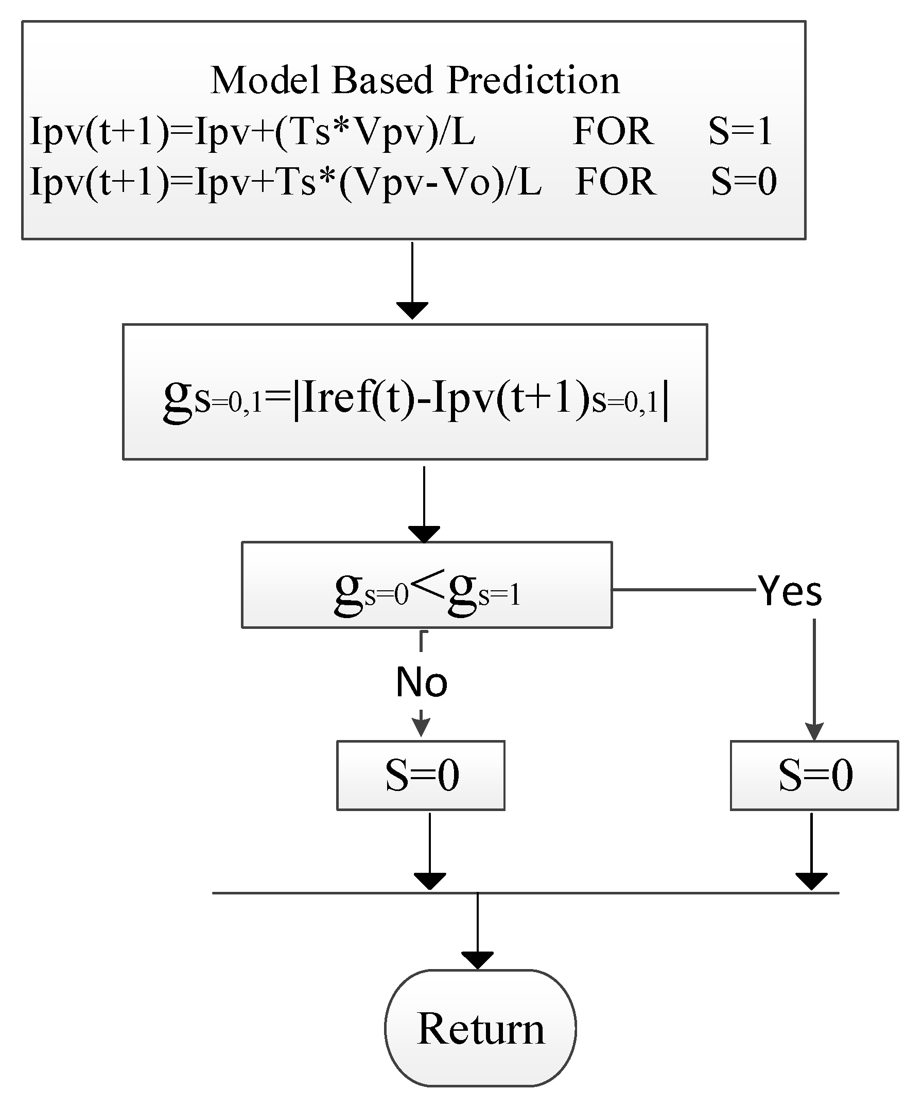
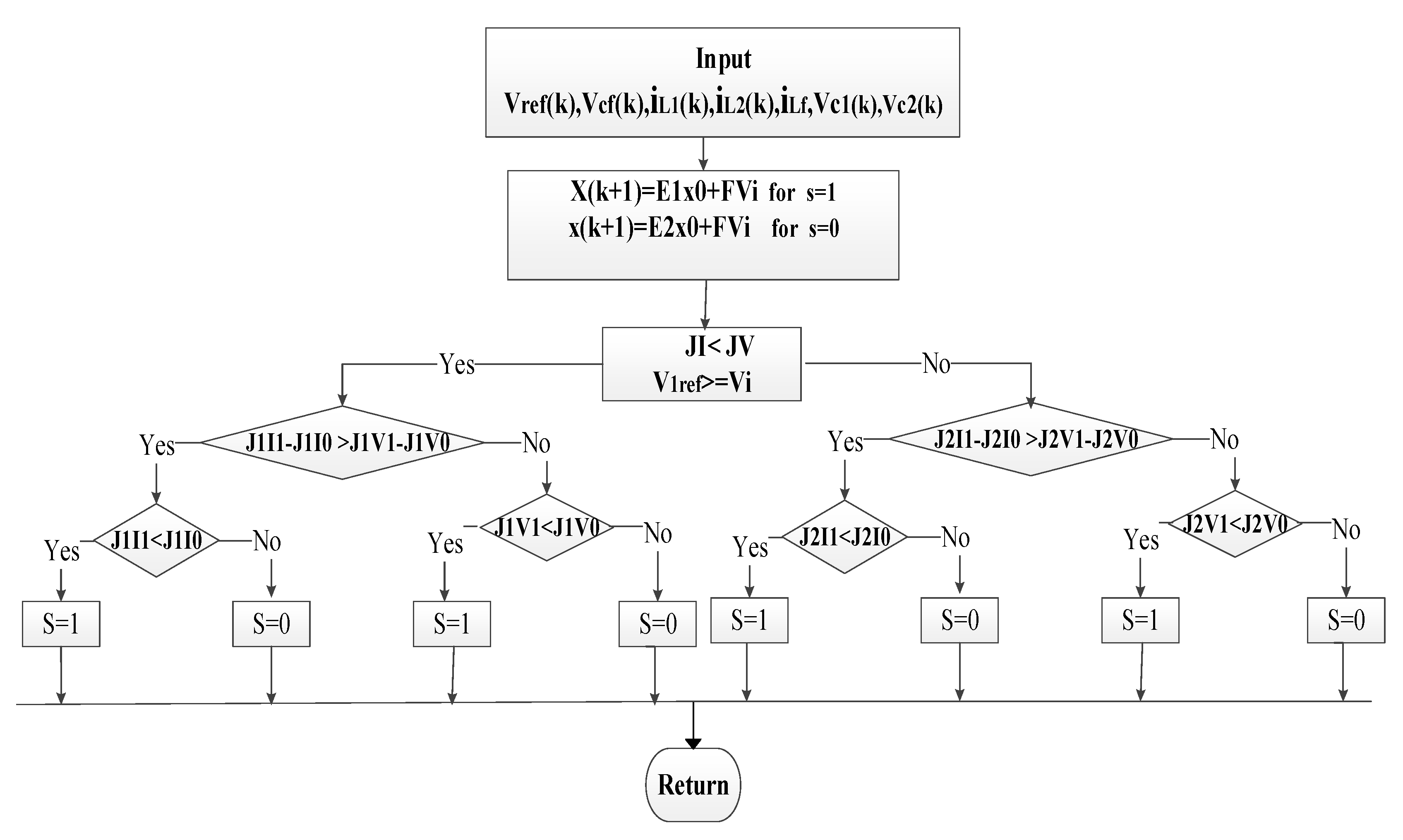
5. Proposed Model Predictive Control (MPC) Strategy

In this section, the MPC algorithm based on the two-error technique is introduced for the single-stage inverter. This algorithm regulates the output voltage by controlling the S1, S4, S2, and S3 switches, and according to the structure of the inverter, its output voltage is equal to:

$$V_o=V_{C1}-V_{C2}$$

(11)

In this equation, V_C1 is the voltage of the first capacitor, and V_C2 is the voltage of the second capacitor. The right leg of the inverter acts as a buck converter, and the left leg acts as a boost converter. We can control the output voltage by controlling the voltages of capacitors C1 and C2.

Objective Function

Equations (12) and (13) represent the objective function of the left foot and the right foot, respectively. In this regard, J1 is the left leg error, and J2 is the right leg error.

$$J1=\{\begin{array}{l}J1I_1=|\frac{(I_{1ref}-i_{L1})}{I_{1ref}}| \stackrel{for}{\to }S=1\\ J1I_0=|\frac{(I_{1ref}-i_{L1})}{I_{1ref}}| \stackrel{for}{\to }S=0\\ J1V_1=|\frac{V_1{}_{ref}-V_{{}_{C1}}}{V_{1ref}}| \stackrel{for}{\to }S=1\\ J1V_0=|\frac{V_{1ref}-V_{{}_{C1}}}{V_{1ref}}| \stackrel{for}{\to }S=0\end{array}$$

(12)

$$J2=\{\begin{array}{l}J2I_1=|\frac{(I_{2ref}-i_{L2})}{I_{2ref}}| \stackrel{for}{\to } S=1 \\ J2I_0=|\frac{(I_{2ref}-i_{L2})}{I_{2ref}}| \stackrel{for}{\to } S=0\\ J2V_1=|\frac{V_{2ref}-V_{{}_{C2}}}{V_{2ref}}| \stackrel{for}{\to }S=1\\ J2V_0=|\frac{V_{2ref}-V_{{}_{C2}}}{V_{2ref}}| \stackrel{for}{\to }S=0\end{array}$$

(13)

In this equation, J1 and J2 are the left and right leg error, respectively, and I_ref and V_ref are the reference current and voltage, respectively. Each error in this mode has four switching modes. The purpose of inverter control is to bring the output voltage to the reference value. In the proposed method, we use both inductor current and capacitor voltage errors. The relationship between the reference current and the reference voltage is as follows:

$$\begin{array}{l}{I}_{1ref}=\frac{Io\times D}{1-D}\\ I_{2ref}=\frac{-Io\times (1-D)}{D}\\ V_{1ref}=\frac{Vi\times D}{1-D}\\ V_{2ref}=\frac{Vi\times (1-D)}{D}\end{array}$$

(14)

$$\begin{array}{l}{I}_o=\frac{V_o}{R_o}\\ D=\frac{V_{ref}}{V_i+V_{ref}}\\ \end{array}$$

(15)

where D is duty cycle, which is obtained by using the reference voltage (V_ref) and the input voltage as in Equation (15). Io is also the output current. Additionally, the reference currents according to the converter dynamics are related to the output voltage in the form of Equation (15). The reference voltage of the capacitors is also related to the input voltage.

The proposed control algorithm works as follows: First, it compares the reference voltage (V_1ref) with the input voltage (Vb). If the reference voltage V_1ref is greater or equal to the input voltage, it applies the switching based on the improvement of the left leg error (J1). In this way, it first compares the difference in inductor current error L1 with the difference in voltage error C1. If the current error is greater, it enters the switch based on the current improvement. If the inductor current L1 has less error in any of the switching modes (0 or 1), that mode is applied to the switch, and if the voltage error is greater than the current error, the switching is applied to the system according to the improvement of the voltage error. Moreover, if the reference voltage V_1ref is less than the input voltage, the switching is applied based on the correction of the right leg error (J2). J2 is switching in the same way as J1. This process continues until the error reaches zero. The block diagram of the predictive control algorithm used in this design for the inverter is shown in Figure 6. Additionally, the inverter parameters are shown in

Table 2. Inverter parameters.

Parameters	Size
Battery voltage (Vb)	100, 120, 90 V
Converter inductance (L1)	0.5 mH
Converter inductance (L2)	0.5 mH
Converter Capacitor (C1)	2 µF
Converter Capacitor (C2)	2 µF
LF	1 mH
Cf	250 µF
Variable resistance (Ro)	95, 190 Ω
Sampling time (Ts)	10 µs

.

6. Simulation Results

The proposed control system is simulated and analyzed using MATLAB software. The values of the parameters are considered with a sampling time of 10 μs. The purpose of the control system is to maintain the output voltage of the converter at the given reference value. The reference voltage is assumed to be equal to 155 V sinusoidal and the simulation time is also 1.5 s. There are three modes of operation, each of which is equal to half a second. The first, second, and third half second of the sun radiation are equal to 700, 1000, and zero W, respectively. Moreover, the amount of battery voltage (Vb) between the boost converter and the inverter in the first, second, and third half second is equal to 100, 120, and 90 V, respectively, and the load resistance in the first, second, and third half second is 190, 95, and 190 Ω, respectively.

Figure 7, Figure 8 and Figure 9 show the voltage, current, and power of the photovoltaic system in three time intervals, indicating that the photovoltaic system is operate at the maximum power point. Figure 9 shows the reference current tracking by the incremental conductivity algorithm and the output current of the panel. As can be seen from the figure, the reference current is synchronized with the output current of the panel in the optimal state by the incremental conductivity algorithm with high accuracy and precision.

The battery is charged during the day, and the battery provides voltage at night. The battery output current in charge and discharge modes is shown in Figure 10.

In the first and second half second, we have the sun radiation, and the battery draws current from the panel and is in charging mode. However, in the third half second, because the radiation is zero, the battery flows to the load and is in discharging mode. When in charging mode, the battery draws 1.1 A from the panel, and in discharge mode, the battery flows 0.7 A to the load.

Figure 11 shows the result of controlling the inverter output voltage by the proposed MPC. Due to the fact that the signal density is high, the simulation is also performed for a time of 0.1 s.

As you can see from Figure 11, the output voltage signal of the inverter is completely sine wave and is equal to the reference value. Now, according to the results obtained from the photovoltaic system simulation, the battery and inverter are analyzed in three simulation time intervals as follows:

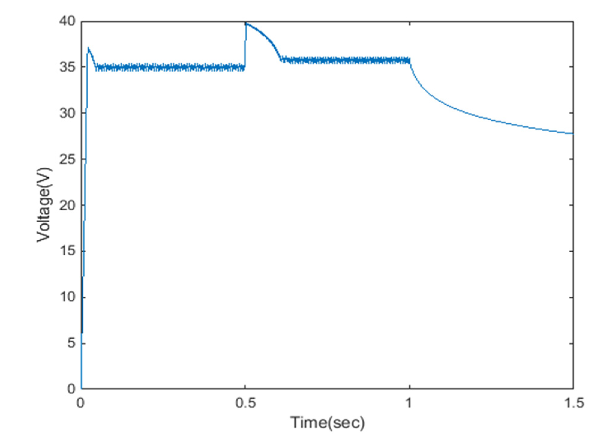
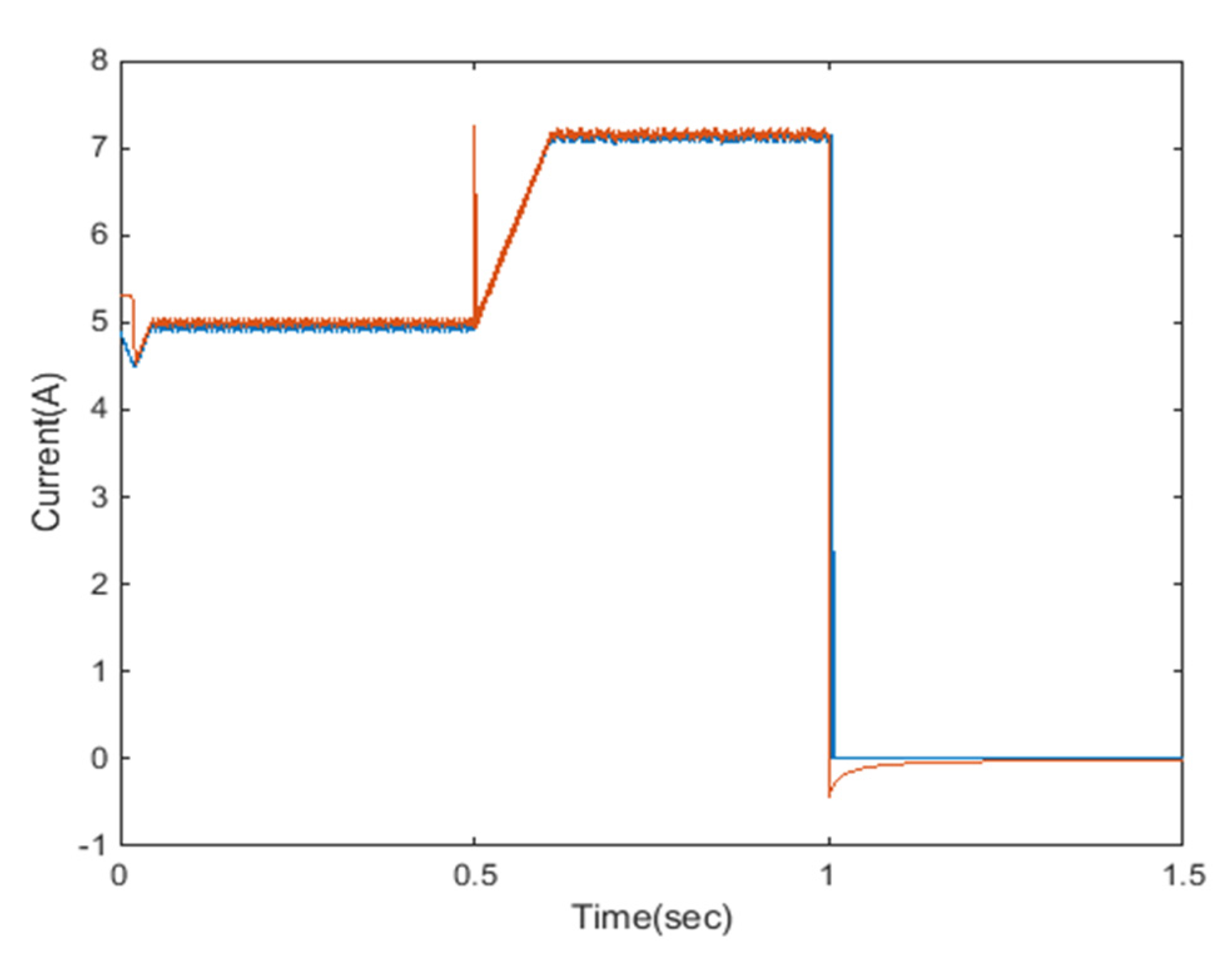
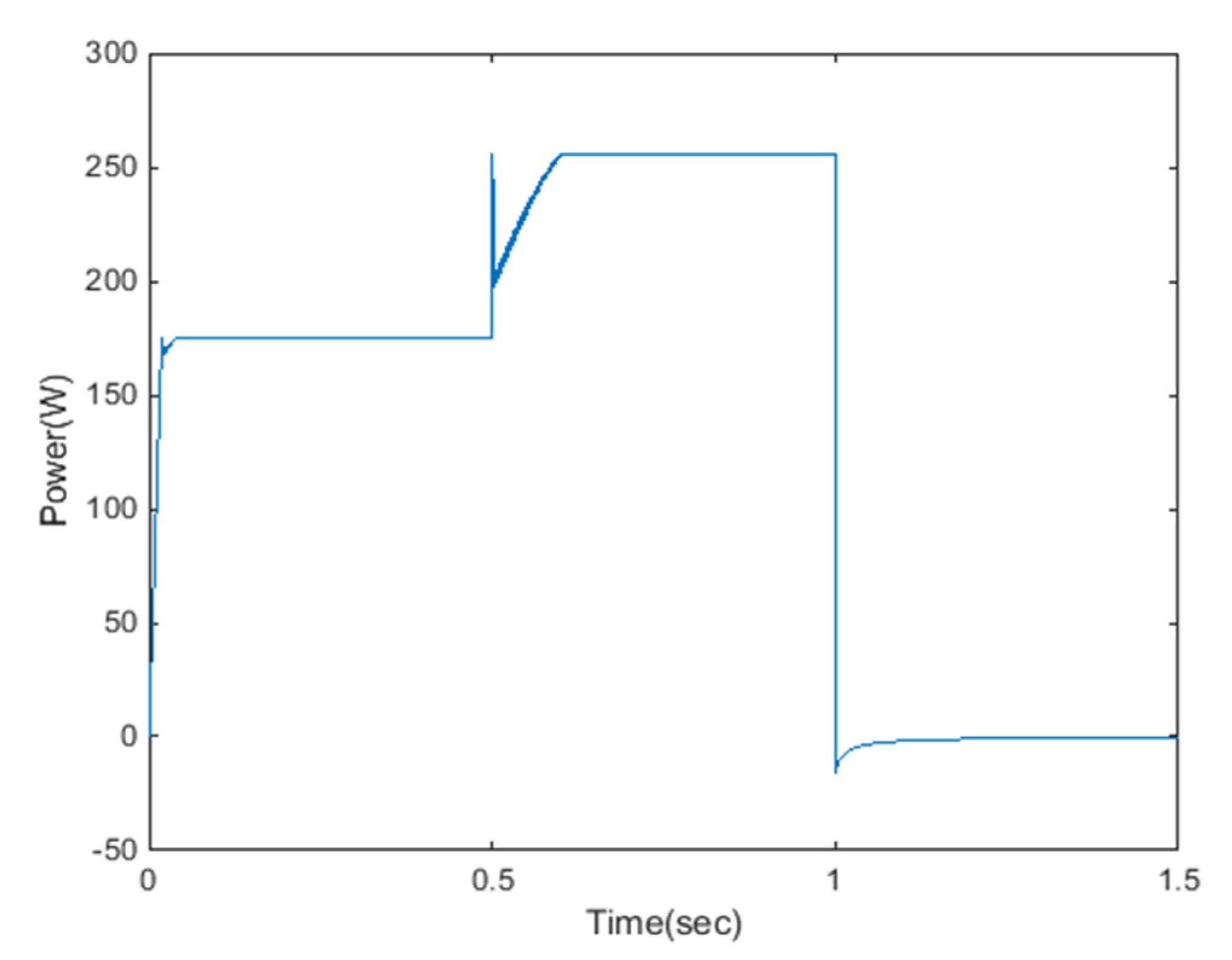
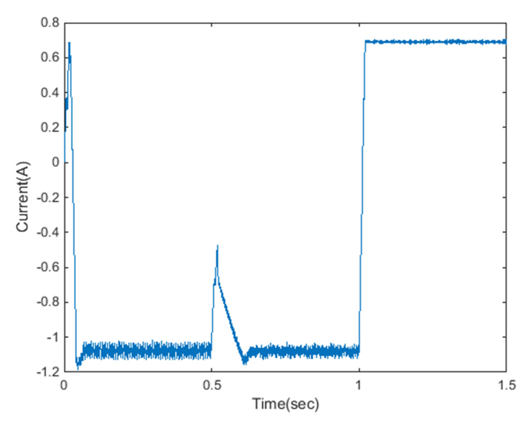
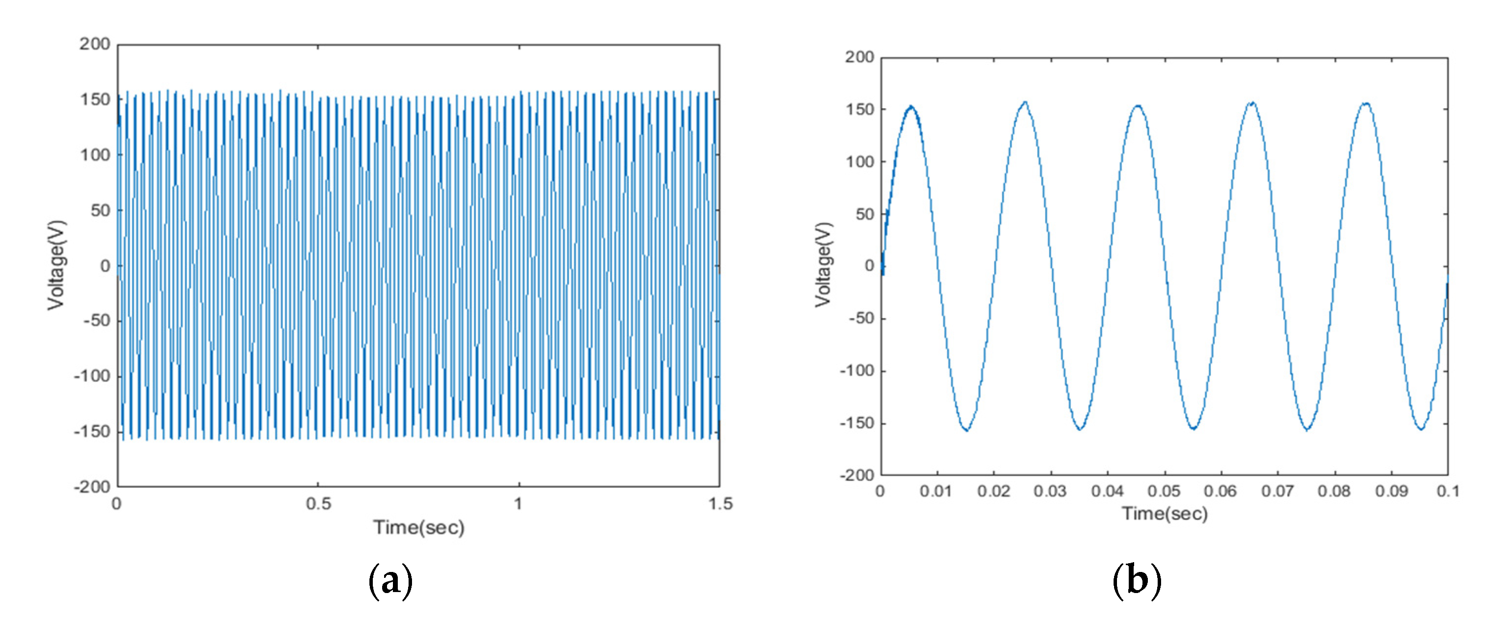
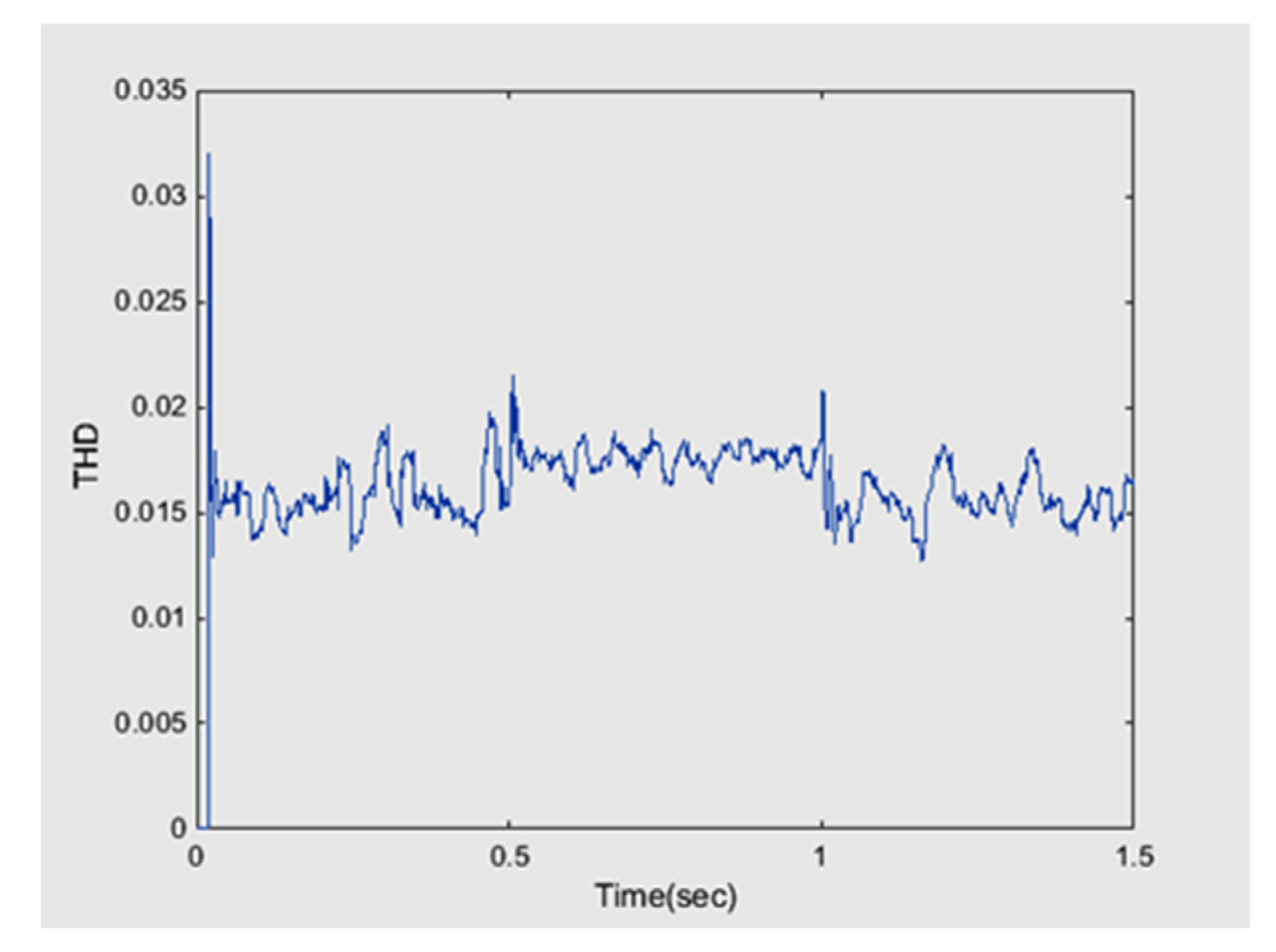
6.1. First Half Second (0 < t < 0.5 s)

This period of solar radiation and ambient temperature are equal to 700 W/m² and 25 °C, respectively, load resistance ro = 190 Ω, and every three half seconds, the reference value of the inverter output voltage is equal to 155 sinusoidal volts. According to the calculations performed in relation (2), the voltage, current, and power of the photovoltaic system are equal to 35 V, 5 A, and 175 W, respectively. As shown in Figure 7, the voltage, current, and power of the panel have reached their optimum values with high speed and accuracy, and this shows that the photovoltaic system operates at the maximum power point, and according to Figure 8, the battery takes about 1.1 A from the panel (in charging mode). During this period, the battery voltage, battery input current, and inverter output voltage are equal to 100 V, 1.1 A, and 155 V, respectively.

Now, using the results obtained from charging and discharging the battery, we obtain the power received from the panel and the power consumption of the load according to the following relations:

$$\begin{array}{l}{\mathrm{P}}_{\mathrm{M}\mathrm{P}\mathrm{P}\mathrm{T}}={\mathrm{P}}_{\mathrm{i}\mathrm{n}}={\mathrm{V}}_{\mathrm{M}\mathrm{P}\mathrm{P}\mathrm{T}}\times {\mathrm{I}}_{\mathrm{M}\mathrm{P}\mathrm{P}\mathrm{T}}\\ {\mathrm{P}}_{\mathrm{i}\mathrm{n}}=35\times 5=175\mathrm{W}\\ {\mathrm{P}}_{\mathrm{B}\mathrm{A}\mathrm{T}}={\mathrm{V}}_{\mathrm{B}\mathrm{A}\mathrm{T}}\times {\mathrm{I}}_{\begin{array}{l}\mathrm{B}\mathrm{A}\mathrm{T}\\ \end{array}}\\ {\mathrm{P}}_{\mathrm{B}\mathrm{A}\mathrm{T}}=100\times 1.1=110\mathrm{W}\\ {\mathrm{P}}_{\mathrm{O}\mathrm{u}\mathrm{t}}={(\frac{{\mathrm{V}}_{\mathrm{O}\mathrm{u}\mathrm{t}}}{\sqrt{2}})}^2/{\mathrm{R}}_{\begin{array}{l}\mathrm{O}\mathrm{u}\mathrm{t}\\ \end{array}}\\ {\mathrm{P}}_{\mathrm{O}\mathrm{u}\mathrm{t}}={(\frac{155}{\sqrt{2}})}^2/190=63\mathrm{W}\end{array}$$

(16)

The photovoltaic system gives us 175 W of power, which stores 110 W in the battery and produces 63 W and has a loss of 2 W.

6.2. Second Half Second (0.5 < t < 1 s)

In a period of 0.5 to 1 s, the sun’s radiation is equal to 1000 W. According to Equation (1), the optimum voltage, current, and power of the photovoltaic system are 35.8 volts, 7.15 A, and 256 W, respectively. According to Figure 7, the voltage, current, and power of the panel have reached their constant value at high speed.

In the second period, according to Figure 8, the battery is receiving power from the panel. As shown in Figure 9, the output voltage of the inverter is equal to the reference value (155 V), and its signal is completely sinusoidal.

According to the current and voltage, the maximum output power of the panel is 256 W. Additionally, the battery voltage, battery input current, load resistance, and inverter output voltage are equal to 120 V, 1.1 A, 95 ohms, and 155 V, respectively. Now, using the results obtained from second half second, we obtain the power received from the panel and the power consumption of the load according to the following relations:

$$\begin{array}{l}{\mathrm{P}}_{\mathrm{M}\mathrm{P}\mathrm{P}\mathrm{T}}={\mathrm{P}}_{\mathrm{i}\mathrm{n}}={\mathrm{V}}_{\mathrm{M}\mathrm{P}\mathrm{P}\mathrm{T}}\times {\mathrm{I}}_{\mathrm{M}\mathrm{P}\mathrm{P}\mathrm{T}}\\ {\mathrm{P}}_{\mathrm{i}\mathrm{n}}=35.8\times 7.15=256\mathrm{W}\\ {\mathrm{P}}_{\mathrm{B}\mathrm{A}\mathrm{T}}={\mathrm{V}}_{\mathrm{B}\mathrm{A}\mathrm{T}}\times {\mathrm{I}}_{\begin{array}{l}\mathrm{B}\mathrm{A}\mathrm{T}\\ \end{array}}\\ {\mathrm{P}}_{\mathrm{B}\mathrm{A}\mathrm{T}}=120\times 1.1=132\mathrm{W}\\ {\mathrm{P}}_{\mathrm{O}\mathrm{u}\mathrm{t}}={(\frac{{\mathrm{V}}_{\mathrm{O}\mathrm{u}\mathrm{t}}}{\sqrt{2}})}^2/{\mathrm{R}}_{\begin{array}{l}\mathrm{O}\mathrm{u}\mathrm{t}\\ \end{array}}\\ {\mathrm{P}}_{\mathrm{O}\mathrm{u}\mathrm{t}}={(\frac{153}{\sqrt{2}})}^2/95=122\mathrm{W}\end{array}$$

(17)

In this case, the photovoltaic system gives us 256 W of power, so the panel can provide load power (122 W) and the excess power output to the battery (132 W). The amount of loss is 2 W.

6.3. Third Half Second (1 < t < 1.5 s)

In the third half second, the radiation is zero (night mode). As you can see from Figure 7, the amount of current and power is equal to zero, and the reason why the voltage is not zero is due to the voltage stored in the capacitor between the boost converter and the panel. Eventually, the voltage is slowly discharged and becomes zero. In the third half second, due to the fact that we do not have radiation, the load power is supplied by the battery. As shown in Figure 10, the battery is discharging and gives 0.7 A to the load. Battery voltage, battery output current, load resistance, and inverter output voltage are 90 V, 0.7 A, 190 Ω, and 155 V, respectively. According to the obtained values, the output power of the system can be obtained according to the following equation:

$$\begin{array}{l}{\mathrm{P}}_{\mathrm{M}\mathrm{P}\mathrm{P}\mathrm{T}}={\mathrm{P}}_{\mathrm{i}\mathrm{n}}={\mathrm{V}}_{\mathrm{M}\mathrm{P}\mathrm{P}\mathrm{T}}\times {\mathrm{I}}_{\mathrm{M}\mathrm{P}\mathrm{P}\mathrm{T}}\\ {\mathrm{P}}_{\mathrm{i}\mathrm{n}}=0\mathrm{W}\\ {\mathrm{P}}_{\mathrm{B}\mathrm{A}\mathrm{T}}={\mathrm{V}}_{\mathrm{B}\mathrm{A}\mathrm{T}}\times {\mathrm{I}}_{\begin{array}{l}\mathrm{B}\mathrm{A}\mathrm{T}\\ \end{array}}\\ {\mathrm{P}}_{\mathrm{B}\mathrm{A}\mathrm{T}}=90\times 0.7=63\mathrm{W}\\ {\mathrm{P}}_{\mathrm{O}\mathrm{u}\mathrm{t}}={(\frac{{\mathrm{V}}_{\mathrm{O}\mathrm{u}\mathrm{t}}}{\sqrt{2}})}^2/{\mathrm{R}}_{\begin{array}{l}\mathrm{O}\mathrm{u}\mathrm{t}\\ \end{array}}\\ {\mathrm{P}}_{\mathrm{O}\mathrm{u}\mathrm{t}}={(\frac{155}{\sqrt{2}})}^2/190=63\mathrm{W}\end{array}$$

(18)

It can be seen that the battery delivers 63 W of power to the load.

The output voltage THD of the inverter is shown in Figure 12:

THD is a qualitative parameter and represents how close a waveform or signal is to a sinusoidal waveform. The amount of THD is expressed as a percentage, and the lower the amount of THD, the better the quality of the sinusoidal waveform. THD less than 5% is acceptable. According to Figure 3, Figure 4, Figure 5, Figure 6, Figure 7 and Figure 8, THD is less than 2%; this means that in the system that has been designed, the output signal is completely sinusoidal and of high quality.

The simulation results show that the output voltage of the inverter has become the same as the reference value with high speed and high quality.

7. Conclusions

In this paper, a system consisting of a photovoltaic system, a DC-DC converter, and a buck-boost inverter is designed. Considering the fact that the maximum efficiency of the solar array should be used when using photovoltaic systems, in this paper, the tracking of the maximum power point has been carried out using the method of incremental conductivity and predictive control. A new method has also been used to control the inverter. This method does not require complex equations, and by simultaneously zeroing the two errors of inductor current and capacitor voltage, with the least calculations, the output voltage reaches the given reference value. The biggest advantage of this method is its simple implementation, and this technique can also be used for DC-DC converters. The purpose of this control system is to produce an output voltage equal to the reference voltage, and according to the simulation results, the inverter output voltage becomes equal to the reference value with high speed and accuracy. Moreover, the total harmonic distortion is less than 2%. As a result, the designed system has a completely sine and high-quality output signal. Finally, it can be seen that using this method, the output voltage of the inverter reaches the specified reference value with high speed and quality. For future research, we can also consider different uncertainties and load variations and analyze their effects. We can also improve this controller by combining the proposed method and other methods, such as artificial intelligence, to deal with the mentioned cases.

References

1. Bolt, G.; Wilber, M.; Huang, D.; Sambor, D.J.; Aggarwal, S.; Whitney, E. Modeling and Evaluating Beneficial Matches between Excess Renewable Power Generation and Non-Electric Heat Loads in Remote Alaska Microgrids. Sustainability 2022, 14, 3884. [Google Scholar] [CrossRef]
2. Hosseini, S.H.; Danyali, S.; Goharrizi, A.Y.; Sarhangzadeh, M. Three-phase four-wire grid-connected PV power supply with accurate MPPT for unbalanced nonlinear load compensation. In Proceedings of the 2009 IEEE International Symposium on Industrial Electronics, Seoul, Korea, 5–8 July 2009; pp. 1099–1104. [Google Scholar]
3. Hosseini, S.H.; Danyali, S.; Goharrizi, A.Y. Single stage single phase series-grid connected PV system for voltage compensation and power supply. In Proceedings of the 2009 IEEE Power & Energy Society General Meeting, Calgary, AB, Canada, 26–30 July 2009; pp. 1–7. [Google Scholar]
4. Mohammadi, F.; Mohammadi-ivatloo, B.; Gharehpetian, G.B.; Ali, M.H.; Wei, W.; Erdinç, O.; Shirkhani, M. Robust Control Strategies for Microgrids: A Review. IEEE Syst. J. 2021, 16, 2401–2412. [Google Scholar] [CrossRef]
5. Tavoosi, J.; Shirkhani, M.; Azizi, A.; Din, S.U.; Mohammadzadeh, A.; Mobayen, S. A hybrid approach for fault location in power distributed networks: Impedance-based and machine learning technique. Electric Power Syst. Res. 2022, 210, 108073. [Google Scholar] [CrossRef]
6. Hu, J.; Zhu, J.; Dorrell, D.G. Model Predictive Control of Grid-Connected Inverters for PV Systems With Flexible Power Regulation and Switching Frequency Reduction. IEEE Trans. Ind. Appl. 2015, 51, 587–594. [Google Scholar] [CrossRef]
7. Danyali, S.; Aazami, R.; Moradkhani, A.; Haghi, M. A new dual-input three-winding coupled-inductor based DC-DC boost converter for renewable energy applications. Int. Trans. Electr. Energy Syst. 2021, 31, 12686. [Google Scholar] [CrossRef]
8. Palanidoss, S.; Thazhathu, S.V.; Bhaskar, M.S.; Kannan, R.; Baboli, P.T. Comprehensive review of single stage switched boost inverter structures. IET Power Electron. 2021, 14, 2031–2051. [Google Scholar] [CrossRef]
9. Huang, H.; Shirkhani, M.; Tavoosi, J.; Mahmoud, O. A New Intelligent Dynamic Control Method for a Class of Stochastic Nonlinear Systems. Mathematics 2022, 10, 1406. [Google Scholar] [CrossRef]
10. Maalandish, M.; Hosseini, S.H.; Sabahi, M.; Asgharian, P. Modified MPC based grid-connected five-level inverter for photovoltaic applications. COMPEL-Int. J. Comput. Math. Electr. Electron. Eng. 2018, 37, 971–985. [Google Scholar] [CrossRef]
11. Silva, J.J.; Espinoza, J.R.; Rohten, J.A.; Pulido, E.S.; Villarroel, F.A.; Torres, M.A.; Reyes, M.A. MPC algorithm with reduced computational burden and fixed switching spectrum for a multilevel inverter in a photovoltaic system. IEEE Access 2020, 8, 77405–77414. [Google Scholar] [CrossRef]
12. Danyali, S.; Moradkhani, A.; Aazami, R.; Haghi, M. New Dual-Input Zero-Voltage Switching DC–DC Boost Converter for Low-Power Clean Energy Applications. IEEE Trans. Power Electron. 2021, 36, 11532–11542. [Google Scholar] [CrossRef]
13. Long, B.; Zhu, Z.; Yang, W.; Chong, K.T.; Rodríguez, J.; Guerrero, J.M. Gradient Descent Optimization Based Parameter Identification for FCS-MPC Control of LCL-Type Grid Connected Converter. IEEE Trans. Ind. Electron. 2022, 69, 2631–2643. [Google Scholar] [CrossRef]
14. Danyali, S.; Niapour, S.K.M.; Hosseini, S.H.; Gharehpetian, G.B.; Sabahi, M. New single-stage single-phase three-input DC-AC boost converter for stand-alone hybrid PV/FC/UC systems. Electr. Power Syst. Res. 2015, 127, 1–12. [Google Scholar] [CrossRef]
15. Tavoosi, J.; Shirkhani, M.; Abdali, A.; Mohammadzadeh, A.; Nazari, M.; Mobayen, S.; Asad, J.H.; Bartoszewicz, A. A New General Type-2 Fuzzy Predictive Scheme for PID Tuning. Appl. Sci. 2021, 11, 10392. [Google Scholar] [CrossRef]
16. Chen, S.; Yang, B.; Pu, T.; Chang, C.; Lin, R. Active Current Sharing of a Parallel DC-DC Converters System Using Bat Algorithm Optimized Two-DOF PID Control. IEEE Access 2019, 7, 84757–84769. [Google Scholar] [CrossRef]
17. Samanes, J.; Urtasun, A.; Barrios, E.L.; Lumbreras, D.; López, J.; Gubia, E.; Sanchis, P. Control design and stability analysis of power converters: The MIMO generalized bode criterion. IEEE J. Emerg. Sel. Top. Power Electron. 2019, 8, 1880–1893. [Google Scholar] [CrossRef]
18. Karamanakos, P.; Liegmann, E.; Geyer, T.; Kennel, R. Model Predictive Control of Power Electronic Systems: Methods, Results, and Challenges. IEEE Open J. Ind. Appl. 2020, 1, 95–114. [Google Scholar] [CrossRef]
19. Palmieri, A.; Rosini, A.; Procopio, R.; Bonfiglio, A. An MPC-Sliding Mode Cascaded Control Architecture for PV Grid-Feeding Inverters. Energies 2020, 13, 2326. [Google Scholar] [CrossRef]
20. Dong, H.; Xie, X.; Zhang, L. A New Primary PWM Control Strategy for CCM Synchronous Rectification Flyback Converter. IEEE Trans. Power Electron. 2020, 35, 4457–4461. [Google Scholar] [CrossRef]
21. Errouissi, R.; Muyeen, S.M.; Al-Durra, A.; Leng, S. Experimental validation of a robust continuous nonlinear model predictive control based grid-interlinked photovoltaic inverter. IEEE Trans. Ind. Electron. 2015, 63, 4495–4505. [Google Scholar] [CrossRef]
22. Sajadian, S.; Ahmadi, R.; Zargarzadeh, H. Extremum seeking-based model predictive MPPT for grid-tied Z-source inverter for photovoltaic systems. IEEE J. Emerg. Sel. Top. Power Electron. 2018, 7, 216–227. [Google Scholar] [CrossRef]
23. Ju, X.; She, C.; Fang, Z.; Cai, T. An improved prediction control strategy of battery storage inverter. In Proceedings of the 2016 IEEE 8th International Power Electronics and Motion Control Conference (IPEMC-ECCE Asia), Hefei, China, 22–26 May 2016; pp. 2047–2051. [Google Scholar]
24. Lopez, D.; Flores-Bahamonde, F.; Kouro, S.; Perez, M.A.; Llor, A.; Martínez-Salamero, L. Predictive control of a single-stage boost DC-AC photovoltaic microinverter. In Proceedings of the IECON 2016-42nd Annual Conference of the IEEE Industrial Electronics Society, Florence, Italy, 23–26 October 2016; pp. 6746–6751. [Google Scholar]
25. Xue, C.; Ding, L.; Li, Y. CCS-MPC with Long Predictive Horizon for Grid-Connected Current Source Converter. In Proceedings of the 2020 IEEE Energy Conversion Congress and Exposition (ECCE), Detroit, MI, USA, 11–15 October 2020; pp. 4988–4993. [Google Scholar]
26. Godlewska, A. Finite control set model predictive control of current source inverter for photovoltaic systems. In Proceedings of the 2018 14th Selected Issues of Electrical Engineering and Electronics (WZEE), Szczecin, Poland, 19–21 November 2018; pp. 1–4. [Google Scholar]
27. Park, S.Y.; Kwak, S. Comparative study of three model predictive current control methods with two vectors for three-phase DC/AC VSIs. IET Electr. Power Appl. 2017, 11, 1284–1297. [Google Scholar] [CrossRef]
28. Islam, H.; Mekhilef, S.; Shah, N.B.M.; Soon, T.K.; Seyedmahmousian, M.; Horan, B.; Stojcevski, A. Performance Evaluation of Maximum Power Point Tracking Approaches and Photovoltaic Systems. Energies 2018, 11, 365. [Google Scholar] [CrossRef] [Green Version]
29. Hosseini, S.H.; Nejabatkhah, F.; Niapoor, S.K.M.; Danyali, S. Supplying a brushless dc motor by z-source PV power inverter with FL-IC MPPT. In Proceedings of the 2010 International Conference on Green Circuits and Systems, Shanghai, China, 21–23 June 2010; pp. 485–490. [Google Scholar]
Figure 1. General schematic of the designed system.
Sustainability 14 11731 g001
Figure 2. Flowchart of incremental conductivity algorithm.
Sustainability 14 11731 g002
Figure 3. Flowchart of maximum power point tracking algorithm using predictive control.
Sustainability 14 11731 g003
Figure 4. Proposed single-stage inverter.
Sustainability 14 11731 g004
Figure 5. Inverter structure in two modes: (a) S1 and S4 switches are on, (b) S1 and S4 switches are off.
Sustainability 14 11731 g005
Figure 6. Flowchart of new two-error predictive control algorithm for single-stage inverter.
Sustainability 14 11731 g006
Figure 7. Photovoltaic panel output voltage.
Sustainability 14 11731 g007
Figure 8. Comparison of MPPT reference current using incremental conductivity and panel output current.
Sustainability 14 11731 g008
Figure 9. Photovoltaic system power.
Sustainability 14 11731 g009
Figure 10. Battery output current.
Sustainability 14 11731 g010
Figure 11. Inverter output voltage for reference 155 V: (a) Simulation time 1.5 s, (b) Simulation time 0.1 s.
Sustainability 14 11731 g011
Figure 12. Inverter output voltage THD.
Sustainability 14 11731 g012