Economic Planning of Energy System Equipment

Abstract

The asset wall (AW) model is widely used by energy companies to forecast the retirement size of equipment. The AW model is a method of arranging historical data in chronological order and then using extrapolation to predict trends in asset size volumes over time. However, most studies using the AW model treat all equipment as a whole and perform a flat extrapolation mechanically, ignoring the impact of technological improvements and price fluctuations. Furthermore, there are relatively few studies on the assetization of equipment replacement scale. This paper fits a Weibull distribution density function and uses Monte Carlo stochastic simulation to determine the retirement age of each piece of equipment, reducing the ambiguity and randomness generated by the AW approach of treating all equipment as a whole. This modified model is noted in this paper as the Weibull–Monte Carlo stochastic simulation asset model wall (WMCAW). The paper then investigated the assetization of equipment replacement size, comparing the three error indicators Mean Absolute Error (MAE), Mean Absolute Percentage Error (MAPE), and Root Mean Square Error (RMSE) in order to select the appropriate optimization model for price forecasting from several combinations of models. Finally, the paper verified the feasibility of the WMCAW model using various types of equipment decommissioned in 1970 and compared the forecasting effects of AW and WMCAW. It is found that the curve of the equipment replacement scale predicted by WMCAW is smoother than that of AW, and the forecasting results are more stable and scientific.

1. Introduction

Most energy companies still belong to the single target or single task type in terms of equipment asset management, focusing on satisfying the operational stability of the equipment and often neglecting asset management issues such as the forecast of the forward replacement scale of the equipment, which will often produce a break in the financial chain in the future. To achieve better refinement of equipment asset management, Alchian [1] first raised the classic “When should current equipment in operation be replaced?”, which unveiled the prelude to the study of equipment replacement in 1952. The replacement of equipment in energy companies has also received a lot of attention in the last two decades. This type of company is typically asset-intensive [2], Xueli Dong et al. (2021) [3] propose solutions to the scale of substation repair and substitution in terms of management systems and cost-cutting. Qu an Zheng et al. (2021) [4] proposed an effective equipment replacement strategy based on lifecycle management (LCC) to ensure that the economic value of old equipment can be fully utilized at the time of decommissioning. Yuxia Peng (2022) [5] proposed a comprehensive technical life evaluation method to provide a basis for the replacement life of energy devices. The literature [1,2,3,4,5] has provided a variety of methods for determining the predicted life of equipment in an energy background, but there is little literature on predicting the scale of facility replacement. Waleed M. Altalabi (2020) [6] mainly used stochastic dynamic programming (SDP), applying a probabilistic approach to study equipment replacement and discussing the operation and maintenance costs while taking into account the price of the equipment by applying inflation and depreciation models to obtain the final forecast size. Carlos Diniz (2021) [7] studied the alignment of strategic plans for equipment commissioning with equipment replacement decisions and developed a mathematical model for the dynamic alignment of strategic plans and replacement sizes, but the model was translated from a forestry context where equipment lifetimes tend to be shorter than tree lifetimes. Liang Wang et al. (2021) [8] researched an accurate decoupling method for SCD files for single device replacement in substations, which reduced the scope of modification and revalidation of SCD files and lowered the change risks associated with SCD modifications. Justyna Sobczak-Piąstka (2021) [9] and others used Visual Basic for Applications (VBA) to obtain several reasonable times for the replacement of equipment to ensure that the equipment was replaced within these life intervals to maximize the value of use. The literature [6,7,8,9] focuses on predicting a reasonable decommissioning life for equipment or suggesting a suitable replacement size for a small number of pieces of equipment. For asset-intensive companies such as energy companies, there is still a lack of research on device replacement, but this type of research work is important in reality. Therefore, it is of great practical importance to carry out research on enterprise equipment asset management and to analyze equipment replacement life, price fluctuations, and technological improvements.

This thesis analyzes the decommissioning situation of each type of equipment, firstly, the annual decommissioning rate of each piece of equipment is corrected using the Weibull distribution, then the Monte Carlo stochastic simulation is performed using the corrected decommissioning rate curve according to the type, respectively. After the simulation, the decommissioning situation of all equipment is summarized and the relevant data are extracted to form the WMCAW model, and finally, the appropriate model is selected for price prediction based on three error indicators, MAE, MAPE, and RMSE, from the combined model composed of the VMD decomposition model, optimization algorithm, and neural network.

This paper adopts a more flexible stochastic simulation, which effectively eliminates the individual stochasticity generated by the leveling extrapolation (mechanically) of the AW model, effectively “peaks averting and valleys filling” for future investment, and effectively reduces the impact of economic factors such as inflation on the model through price forecasting. As the assets of energy companies become larger and larger, requiring huge amounts of capital to maintain the stable operation of equipment, single-tasking system work is no longer applicable to existing energy companies. WMCAW, however, can reasonably forecast the scale of equipment replacement in the long term, playing a key role in ensuring the stability of the capital chain and achieving sustainable development of the energy company’s equipment.

2. Research Methods

The Weibull distribution is mainly used to predict the reliability life of various components and equipment and is the theoretical basis for reliability analysis and life testing. For example, Miu (2021) [10] used the Weber distribution to obtain the reliability function and calculated the remaining life of the key parts of the infant incubator; Wang (2019) [11] fitted the Weber distribution parameters to estimate the average life of the power meter by calculating the expectations of the Weber distribution; Teng (2021) [12] obtained the hybrid Weber distribution and studied the reliability of the power meter by classifying the fault tree of the power meter and fitted the Weber distribution according to the type of fault.

The Weibull distribution is a continuous probability distribution and the expression of its probability density function is defined by:

$$f(t)=\frac{\mathsf{\beta }}{\mathsf{\eta }}{(\frac{t-\mathsf{\gamma }}{\mathsf{\eta }})}^{\mathsf{\beta }-1}{e}^{-{(\frac{t-\mathsf{\gamma }}{\mathsf{\eta }})}^{\mathsf{\beta }}},\mathsf{\beta }>0,\mathsf{\eta }>0,\mathsf{\gamma }>0$$

(1)

where t is the free variable, $\mathsf{\eta }$ is the scale parameter, $\mathsf{\beta }$ is the shape parameter, and $\mathsf{\gamma }$ is the position parameter.

The Weber distribution is divided into three parameters and two parameters. Among them, Li (2022) [13] introduced the three-parameter Weber distribution, and the commonly used methods for fitting the Weber distribution parameters were: moment estimation, L estimation, and maximum likelihood estimation. This article comprehensively compared these three methods. Through the analysis and comparison of curve diagrams of deviation and mean square error changes, it was concluded that the L estimation method had the best performance, followed by the conclusion of maximum likelihood estimation and the worst performance of the moment estimation method.

The distribution function of the three-parameter Weibull distribution is defined by:

$$F(t)=\left\{\begin{array}{l}{1-e}^{-{(\frac{t-\mathsf{\gamma }}{\mathsf{\eta }})}^{\mathsf{\beta }}},t\ge 0\\ 0\hspace{1em}\hspace{1em},t < 0\end{array}\right.$$

(2)

When the equipment holds the possibility of being retired in the first year with $\mathsf{\gamma }=0$, then the three-parameter Weibull distribution is converted to a two-parameter Weibull distribution that only contains $\mathsf{\beta },\mathsf{\eta }$.

Assuming that the three-parameter Weibull distribution degenerates to a two-parameter ($\mathsf{\beta },\mathsf{\eta }$)Weibull distribution, the commonly used parameter fitting methods are least squares and great likelihood estimation. Wen (2021) [14] used the least square method to derive the distribution function of Weber distribution, and then the life expectancy probability of the electric submersible pump was obtained, and the probability of each possible retirement life was analyzed, taking the least squares method as an example.

After shifting the terms of Equation (2) according to the rules of calculation, we get:

$$1-F(t)=e^{-{(\frac{t}{\mathsf{\eta }})}^{\mathsf{\beta }}},t\ge 0$$

(3)

Equation (3) can be performed with a continuous logarithmic transformation to obtain:

$$\ln (\ln \frac{1}{1-F(t)})=\mathsf{\beta }\ln t-\mathsf{\beta }\ln \mathsf{\eta }$$

(4)

Let $Y=\ln (\ln \frac{1}{1-F(t)}),x=\ln t$, (4) can be expressed as follows:

$$Y=\mathsf{\beta }x-\mathsf{\beta }\ln \mathsf{\eta }$$

(5)

Let $\mathsf{\beta }=B,A=\mathsf{\beta }\ln \mathsf{\eta }$, the least squares fit to Equation (5).

$$\widehat{B}=\frac{l_{xY}}{l_{xx}},\widehat{A}=\overline{Y}-\mathsf{\beta }\overline{x}$$

With $\mathsf{\beta },\mathsf{\eta }$ h $l_{xx}={\displaystyle \sum _{i=0}^n{(x_i-\overline{x})}^2},l_{xY}={\displaystyle \sum _{i=1}^n(Y_i-\overline{Y})(x_i-\overline{x})}$.

The estimated value can be obtained after the restorations of $\widehat{A},\widehat{B}$ have been given.

2.1. Asset Wall

Asset wall (AW) is an application of the time series forecasting method. It is a quantitative forecasting method that arranges historical data into a time series in chronological order, then analyzes its change trend over time for extrapolation. It is based on the historical data arranged in chronological order and then analyzes the regular pattern of its changes over time, finally taking the time of commissioning as the horizontal axis and the scale of asset value as the vertical axis, which shows the scale of assets in operation in the shape of a “wall”, reflecting the scale of existing assets in operation for different years in history.

The extrapolation of AW combined with the translation life can predict the future equipment decommissioning of the existing assets. For example, Sun (2015) [15] obtained the original value or retirement scale of the future asset transformation of individual assets through the translation (actual service life) of the unit asset wall and then accumulated the overall asset wall of the future company to predict the scale of future technological transformation. The leveling years N can be the average service life, design life, economic life of the equipment, etc. The total physical wall can be established by adding up the statistics of various historical assets in operation, which has reference value for predicting the value scale and investment scale of future equipment retirement. AW can also be combined with other algorithms to achieve prediction. For example, Shi (2018) [16] combined the “asset wall” with the “inefficiency” curve to infer the peak period of operation and maintenance workload. Li (2019) [17] combined the “asset wall” model with the full life management (LCM) theory to obtain more economical and accurate investment forecasts.

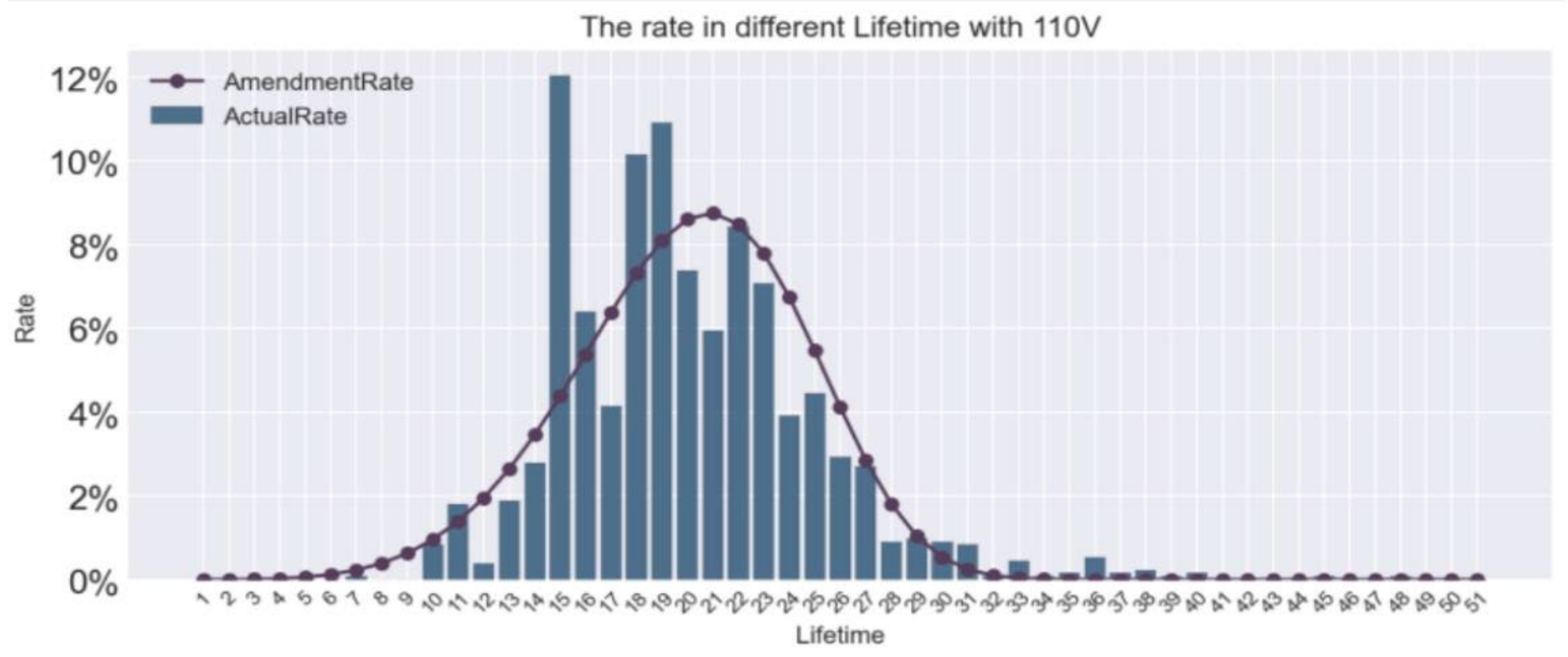
Figure 1 shows the analysis of a power company’s 110 KV transformer in-operation equipment using the AW model to predict the scale of device retirement of the stock assets.

Figure 1 is the result of smoothing according to the design life of a 110 KV transformer. According to the curve fluctuation, we can know that the peak of equipment commissioning would be ushered in around 2016 and 2018; the peak of equipment retirement will be ushered in around 2056 and 2058, correspondingly, so the fund scheduling can be carried out in advance to prevent the shortage of funds during the peak period of device decommissioning.

2.2. Monte Carlo Simulation (MC)

MC is also called the randomized test or statistical test method. V.A. Shneidman (1999) [18] first used MC to carry out the large-scale MC and theoretical analysis of small clusters and large nuclei on two-dimensional Ising lattices, verifying the dynamic and thermodynamic properties of several mainstream nucleation methods. The basic principle of the method is based on obtaining the frequency of events through some kind of large number of tests, which can be used as the solution to the problem according to the law of large numbers. MC solves various problems by constructing random numbers that conform to certain rules. It is an effective method for solving quantitative problems that are difficult to obtain results from and hold large uncertainty due to excessive computational complexity. For example, Rjiba Abdelkarim (2021) [19] used MC and the nearest neighbor method to study the structural properties of LiCl saline solution under environmental conditions; Zhang Y et al. (2022) [20] proposed a set of interval prediction schemes that can accommodate wind speeds with different error characteristics based on Monte Carlo theory; Lee Jae Ha (2021) [21] investigated the pharmacokinetics (PK) of meropenem, a severe adult patient receiving in vitro membrane oxygenation (ECMO), and used the MC to evaluate the probability of achieving the goal and determine the appropriate dose scheme; the literature [22,23] used MC to obtain the reliable life of equipment; in the context of the new electrical transformation, Wu (2018) [24] calculated the probability distribution of various risk variables that affect investment risk, used MC to obtain the net present value prediction model diagram, and observed the probability of each return level through the graph, so as to judge the feasibility of investment. Wang (2018) [25] refined the hierarchy of various uncertain influencing factors through the AHP and used MC to determine the probability distribution of net present value.

Since MC is an idea, the specific algorithm of the simulation needs to be analyzed according to the specific problem. The following are the specific steps for applying the MC methodology to the physical asset management of an energy company.

Step 1: Refine the equipment types, the voltage levels of each type, and collect data on all historical equipment put into operation by energy companies, including the years of operation of each piece of equipment, the life span of retired equipment, and the number of pieces of equipment in operation.

Step 2: Analyze the data of historical decommissioned equipment, calculate the decommissioning probability for each type of equipment for each decommissioning period, and take it as the assignment probability of MC.

Step 3: Count the number of pieces of equipment in operation for each type, perform MC for each piece of equipment in Step 2, and count the number of future years of decommissioning after simulation for all equipment to form a predicted equipment-decommissioning quantity wall for that type.

Step 4: Repeat the random simulation ten times, take the average value of the quantity of each year in the quantity wall, and make statistics again to form the device retirement quantity wall.

2.3. Variational Modal Decomposition (VMD)

Wavelet variation as a classical data processing method suffers from the problem that the wavelet basis function cannot change adaptively. To solve this problem, H. E. Huang (1998) [26] proposed a groundbreaking empirical modal decomposition algorithm (EMD), which was based on the characteristics of the original signal itself and was used without pre-research on the signal, decomposing the signal according to different requirements, decomposing the signal into several modes, and taking its decomposition results. It was a series of signal component modes with relatively fixed fluctuation periods with good physical characteristics. Its algorithm advantages were mainly reflected in the processing ability of nonlinear and non-stationary signals. The EMD algorithm breaks the traditional idea of defining frequency and successfully gives a description of the essential image of the signal. This method has been successfully applied to power load prediction, fault diagnosis, bridge fault monitoring, and other engineering fields. However, EMD also has an obvious drawback: in the case of the original signal having local large fluctuations, it is difficult for EMD to separate this feature. This problem is called the modal conflation problem. In WT and EMD with endpoint effects and modal confusion, the choice of wavelet function will directly affect the prediction accuracy. Zhang Y and others (2022) [27] tried to improve the EMD to solve this problem and scholars have proposed improvement algorithms such as the ensemble empirical modal decomposition (EEMD). In response to the problem of the incomplete noise removal of the EEMD method, the CEEMD method was proposed in 2011.

Variational Mode Decomposition (VMD) is a novel modal decomposition algorithm, proposed by Dragomiretskiy K et al. in 2013, which can effectively solve the modal mixing problem that occurs when the empirical mode decomposition (EMD) decomposes the original signal. Zhang Na (2022) [28] and others believed that VMD was a completely non-recursive signal variation and signal processing method that provided a practical method for processing non-stationary signals. Zhang Y. et al. (2022) [29] concluded that the VMD method can fully extract the linear and nonlinear features of the data and give full play to the advantages of different numerical prediction methods, which can significantly improve the performance of the prediction model and increase the prediction accuracy. Han Yu et al. (2022) [30] proposed that compared with the uncertainty of the number of modal components in the process of EMD algorithm decomposition, the VMD method can artificially specify the number of modal decompositions, and the determination of modal numbers of the VMD method was subjective, which affected the reliability of signal decomposition. Compared with the EMD algorithm, VMD has a more solid mathematical theoretical foundation. By a given number of decompositions, VMD can separate each intrinsic mode (IMF) by solving the optimal solution of the variational problem. Its decomposed IMFs have higher stationarity, which can better extract the information from the time series in carbon price forecasting and help to improve the forecasting effect.

VMD requires the construction of the variational problem of the signal, letting the original signal $\phi$ be decomposed into n modal components of definite frequency and finite bandwidth. The constraint is the sum of the modal components for the original signal; the optimal solution of the solution is the minimum sum of the bandwidth of each mode. The mathematical expression of the variational problem is:

$$\left\{\begin{array}{l}\underset{\left\{IM{F}_n\right\},\left\{{\omega }_n\right\}}{\min }\left\{{{\displaystyle \sum _n‖{\partial }_t\left[\left(\delta \left(t\right)+\frac{j}{\pi t}\right)\times IM{F}_n\left(t\right)\right]\times e^{-j{\omega }_{n}t}‖}}_2^2\right\}\\ s.t.{\displaystyle \sum _{n}IM{F}_n=\phi }\end{array}\right.$$

(6)

where $\left\{IM{F}_{\mathrm{n}}\right\}$ is the decomposed n modes and $\left\{{\omega }_n\right\}$ is the center frequency corresponding to each mode component. The decomposition of the variational mode is done by circular iteration and the final optimal solution is the solved variational mode.

2.4. Elman Neural Network

The BP neural network is one of the most basic neural networks, its backpropagation characteristic has a good effect on predicting nonlinear sequences. Chunzhi Wang (2021) and others [31] believed that the BP neural network was a neural network with forward signal propagation and error reverse propagation. It is mainly composed of three neuron layers, namely, the input layer, the hidden layer, and the output layer. The neurons between the layers are connected and the neurons within the layers are not connected. Yu Yuge et al. (2020) [32] proposed that the BP neural network belonged to the forward neural network, which was characterized by the addition of a reverse propagation algorithm. The core of the algorithm was to transmit the difference from the back to the front when the value of the network output deviated from the actual value. The weights of each layer of the network are adjusted in the direction of reducing the deviation to achieve the full purpose of the adjustment. After continuous forward and reverse adjustment, the deviation is reduced to the expected range. If the parameters are not selected correctly when using a neural network model, it can lead to too many training iterations or non-convergence. Zhang Y et al. (2020) [33] proposed the EPSO optimization method, which integrates the optimization ideas of the extreme value optimization (EO) algorithm into the PSO algorithm to solve this problem. However, the structure of the BP neural network is relatively simple, so it has poor performance in predicting more complex data. In addition, the BP neural network does not have the ability to remember the historical changes to the data and may ignore the information contained in it. Therefore, its carbon price prediction results are more inaccurate and less stable. To address these problems, the Elman neural network is chosen as a prediction tool instead of the BP neural network in this paper.

Liu B et al. (2021) [34] proposed that Elman neural network was a multi-level dynamic neural network. Due to its dynamic recursive structure, it has a good approximation ability for nonlinear functions. Compared with the BP neural network, the Elman neural network adds a takeover layer on top of the hidden layer. The takeover layer can record the output results of the hidden layer in the last training and pass the recorded information into the hidden layer in the current training. This connection enables the network to enjoy memory function, thus improving the network’s ability to process dynamic information. This improvement effectively improves the prediction ability of the neural network, making it possible to carry out the short-term memory of the historical change information of time series. Zhang Y and Chen Y (2021) [35] proposed that Elman improved by BP not only has the ability to handle large-scale data but also has good results in prediction by its local memory unit and local feedback connection. In addition, compared with complex deep learning algorithms, the structure of the Elman neural network is relatively simple and the prediction speed is faster. The forward training formula of the Elman neural network is as follows:

$$\begin{array}{l}x\left(k\right)=f\left({\omega }_1{x}_c\left(k\right)+{\omega }_{2}u\left(k-1\right)\right);\\ x_c\left(k\right)=\alpha x_c\left(k-1\right)+x\left(k-1\right);\\ y\left(k\right)={\omega }_{3}x\left(k\right)\end{array}$$

(7)

where $x\left(k\right)$ is the output value of the hidden layer, $x_c\left(k\right)$ is the output value of the take-up layer, $y\left(k\right)$ is the output value of the output layer, and $u\left(k-1\right)$ is the input value of the input layer. ${\omega }_1,{\omega }_2,{\omega }_3$ are the corresponding weights. $\alpha$ determines whether the context layer remembers the result of the last take-up; if $\alpha =0$, then the neural network is a standard neural network.

2.5. Gray Wolf Optimizer (GWO)

Many optimization algorithms are inspired by animals in nature, such as particle swarm algorithms imitating birds and bee swarm optimization algorithms that mimic bees, etc. The gray wolf optimizer (GWO) is a novel bionic optimization algorithm invented by scholar Mirjalili in 2014, whose algorithm imitates wolves’ predation. GWO is favored by scholars in many fields and is widely used in parametric optimization because of its simple structure, few parameters, and fast convergence speed.

Hou Yongyan (2022) [36] and others believed that the gray wolf optimization algorithm was a new metaheuristic search algorithm that simulated the social hierarchy structure and prey process of gray wolves in nature. The basic idea is to use the position vector of each individual wolf in the wolf pack to represent the parameters to be optimized, introduce a leader strategy to simulate the process of wolf pack surrounding and preying, treat the ideal optimal parameter value as the position of the prey, and complete parameter optimization.

Wolves in packs are highly social animals and the population is divided into multiple classes. Therefore, GWO also divides the search units in the algorithm into four classes: a, b, and c wolves representing the ruling class, which are composed of the top three wolves with the highest adaptation level in the pack, and d wolves, representing the commoner class, which consists of all the remaining wolves in the pack. In reality, the wolves will gradually surround the prey, and in the GWO algorithm, the process of surrounding the prey is expressed by Equation (8):

$$\begin{array}{l}D=\left|C\cdot X_h\left(t\right)-X\left(t\right)\right|\\ X\left(t+1\right)=X_h\left(t\right)-A\cdot D\end{array}$$

(8)

where $X\left(t\right)$ is the position of the wolves at the current moment. $X_h\left(t\right)$ is the position of the prey at moment t, and $A,C$ are the search coefficients, determined as follows:

$$\begin{array}{l}A=2a\cdot r_1-a\\ C=2\cdot r_2\end{array}$$

(9)

where $a$ is the shrinkage factor, which decreases linearly with the iteration, and $r_1,r_2$ is the random factor, whose random range is between [0, 1]. The addition of the random factor improves the randomness of the algorithm, which can effectively improve the global search ability of the algorithm and reduce the possibility of the algorithm falling into local optimal solutions.

The gray wolf algorithm is characterized by the possibility of $a,b,c$, three ruling wolves, directing the $d$ wolves to move and search for prey, a process that can be represented by the following equation:

$$\left\{\begin{array}{l}{D}_a=\left|C_a\cdot X_a-X_d\left(i\right)\right|\\ D_b=\left|C_b\cdot X_b-X_d\left(i\right)\right|\\ D_c=\left|C_c\cdot X_c-X_d\left(i\right)\right|\end{array}\right.$$

(10)

$$\left\{\begin{array}{l}{X}_1=X_a-A_a\cdot D_a\\ X_2=X_b-A_b\cdot D_b\\ X_3=X_c-A_c\cdot D_c\end{array}\right.$$

(11)

$$X_d\left(i\right)=\frac{\left(X_1+X_2+X_3\right)}{3}$$

(12)

where $D_1,D_2,D_3$ represents the distance between the ith wolf in $\mathrm{d}$ wolves and the three wolves in a, b, c. Factor $A_{1,2,3},C_{1,2,3}$ is generated in the same way as Equation (11).

The gray wolf recognized the location of the prey and surrounded the prey. When the position of the prey stopped moving, the gray wolf group will complete the hunting by gradually reducing the scope of the siege. (Zhang Na and others, 2022) [26].

In summary, the iterative search process of GWO is as follows:

Step 1: Initialize the function to randomly generate the positions of all wolves in the wolf pack.

Step 2: Calculate the fitness of each wolf and determine wolves a, b, c, and d according to their fitness.

Step 3: Update the contraction factor and the random factor.

Step 4: According to Equations (10)–(12), let wolves a, b, and c command the wolves to move and obtain the new position of the wolves.

Step 5: Iterate steps 2–4 until the search is reached or the maximum number of iterations is reached, then stop the algorithm.

3. Empirical Analysis—Taking a 220 kV Transformer and 110 kV Circuit Breaker as Examples

Since there are many power companies in the energy system, in this paper, we extracted data from a power company and selected two types of representative physical assets, 220 KV transformers and 110 KV circuit breakers, respectively. Through the empirical analysis of these two types of equipment, the feasibility of the improved “asset wall” model is demonstrated.

3.1. Correction of Actual Equipment Decommissioning Rate Using Weibull Distribution

3.1.1. Data Acquisition and Processing

According to the Enterprise Resource Planning (ERP) data of this power company, the information related to retired equipment is first derived according to the type of equipment and then according to each voltage level, which includes the years of commissioning of retired equipment, the years of retirement of retired equipment, the years of use, and the reasons for retirement. Then, we may analyze the situation of the equipment that has been retired and count the actual years of retirement of various types of equipment.

Due to the long life of the physical assets and equipment, most of the equipment put into operation in the past two decades is still in operation. For the convenience of statistical analysis, the following research is conducted with the equipment put into operation in 1970 (most of the equipment put into operation in 1970 is decommissioned).

In this paper, 100 transformers were randomly sampled from the decommissioned equipment put into operation in 1970, and the decommissioning rate of each year was calculated according to the decommissioning life of each unit. The actual decommissioning rate of 220 KV transformers and 110 KV circuit breakers in each year is shown in Figure 2 and Figure 3.

From Figure 2, in the 10th year, the 220 KV transformers began to be decommissioned, and the 16th–23rd years were at the peak of decommissioning. After that, the de-commissioning rate began to show a downward trend. In the 40th year, almost all the equipment was decommissioned.

From Figure 3, in the 8th year, the 110 KV circuit breakers began to be decommissioned. In the 15th to 24th year, they were at the peak of decommissioning, and in the 44th year, the equipment was basically fully decommissioned.

3.1.2. Fitting of the Weibull Distribution Parameters

The fitted Weibull distribution is corrected by the actual decommissioning rate of the decommissioned equipment for each year, in preparation for subsequent MC.

Taking the 220 KV transformer as an example, for Equation (13), $t$ is represented by $t_{\left(i\right)}$, for 1000 data arranged according to the length of the retirement life, a total of 1000, define $M_{\left(i\right)}$ as the sample with serial number $i$ in this sample and $t_{\left(i\right)}$ as the length of the retired life of the sample. Then:

$$1-F(t_{(i)})=e^{-{(\frac{t_{(i)}}{\mathsf{\eta }})}^{\mathsf{\beta }}}$$

(13)

where $F(t_{(i)})$ is the median rank and is calculated as $F(t_{(i)})=\frac{i-0.3}{n+0.4},n=1000$.

The transformation gives:

$$\ln (\ln \frac{1}{1-F(t_{(i)})})=\mathsf{\beta }\ln (t_{(i)})-\mathsf{\beta }\ln \mathsf{\eta }$$

(14)

The least squares fitting of observation $(t_{(i)},F(t_{(i)}))$ of group 1000 $M_{(i)}$ to Equation (14) yields $\mathsf{\eta },\mathsf{\beta }$ for the 220 KV transformer.

$$\mathsf{\eta }=21.78,\mathsf{\beta }=5.08$$

(15)

Substitute $\mathsf{\eta },\mathsf{\beta }$ into Equation (1) to obtain the Weibull distribution density function. The result is shown in Figure 4, in which the curve is the fitted Weibull curve of the 220 KV transformer decommissioning rate.

As can be seen from Figure 4, the curve showed a trend of “low at both ends and high in the middle”, in which the decommissioning rate was almost 0% in the first 5 years, peaked in the 22nd year, and then decreased linearly to 0% in the 33rd year. Except for a slight difference in the curve at the peak year, the rest of the curve was fitted intact.

Similarly, repeat the above operation for the 110 KV circuit breakers to obtain $\mathsf{\eta },\mathsf{\beta }$.

$$\mathsf{\eta }=23.19,\mathsf{\beta }=4.23$$

(16)

Figure 5 shows the Weibull curve fitted to the 110 KV circuit breaker retirement rate.

The actual decommissioning rate of 110 KV breakers was more scattered. When fitting the Weibull distribution, it can be seen in Figure 5 that there was a gap between the curve situation and the actual situation in the peak period; the actual decommissioning rate was higher in years 33–38, and the fitted value of the curve was lower. The rest of the fit is good except for each individual value.

Figure 4 and Figure 5 provided promising simulations, the Weibull-corrected decommissioning rate for each year will be used in MC to determine the decommissioning age of each unit.

3.2. Establish a Quantitative Wall

Based on the ERP data of the power company, the data of all the equipment in operation were first derived according to the type of equipment and then according to each voltage level, and the number of equipment was summed up based on the same year of operation to form a quantitative wall. The purpose of establishing the quantitative wall is to have an image of the operation scale of the existing equipment in operation each year and to deduce the future retirement peak based on the asset wall, so as to make capital dispatch in advance and prevent capital chain breakage.

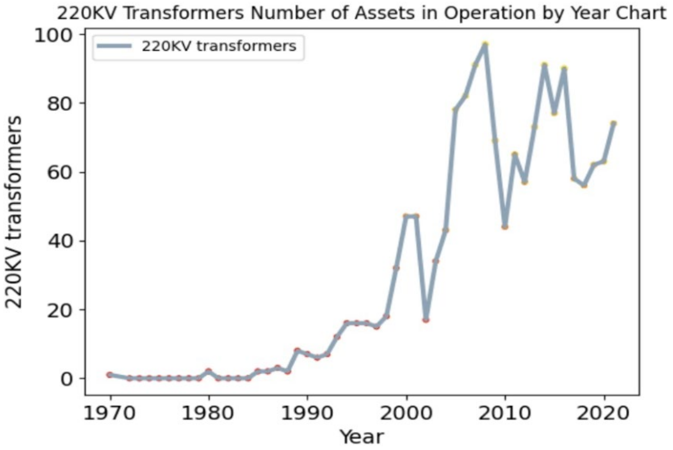
Figure 6 and Figure 7 are the quantity wall diagrams of 220 KV transformers and 110 KV circuit breakers, respectively.

According to the statistics, there were a total of 1580 transformers in operation at 220 KV. Figure 6 shows that there was almost no more equipment in operation from 1970 to 1983. The number of pieces of equipment in operation since 1985 and still in operation has shown a rapid upward trend, peaking in 2008. Since the number of pieces of equipment in operation was also closely related to the amount of equipment in operation in that year, when the amount of equipment in operation declined from 2009 to 2012, it can be observed that the number of pieces of equipment in operation also showed a decreasing trend. Since 2013, the number of shipments has again entered a period of rapid increase, but the highest point is almost the same as in 2008.

According to the statistics, there are 2838 circuit breakers in operation at 110 KV. According to Figure 7, the amount of equipment in operation before 1994 was low, and almost all the equipment in operation has been retired. Since 1995, the number of shipments has risen sharply, peaking at 431 around 2008, and then plummeting. In 2021, it was the lowest point in nearly 20 years, at 22, which is closely related to the significant reduction in 110 KV circuit breakers input since 2009.

3.3. Using MC to Analysis the Example

Figure 8 draws an MC flowchart with 220 KV transformers as an example, and the process of building other equipment is similar. The rest of the energy system’s physical assets can also be built according to this method of a quantitative wall.

The specific rules for utilizing MC for a single piece of equipment are as follows.

Step 1: Integrate the Weibull-corrected decommissioning years, because the probability of decommissioning life exceeding 40 years is low, so when conducting the stochastic simulation, all the service lives of equipment that may exceed 40 years are considered according to 40 years. Taking 220 KV transformers as an example,

Table 1. Weibull-modified decommissioning rate by year of 220 KV transformers.

Decommissioning Service Life	Retirement Rate	Decommissioning Service Life	Retirement Rate
1	0.000081%	21	8.8%
2	0.0014%	22	8.5%
3	0.0071%	23	7.8%
4	0.023%	24	6.7%
5	0.057%	25	5.5%
6	0.12%	26	4.1%
7	0.23%	27	2.9%
8	0.39%	28	1.8%
9	0.63%	29	1.0%
10	0.95%	30	0.53%
11	1.4%	31	0.24%
12	2.0%	32	0.10%
13	2.6%	33	0.033%
14	3.5%	34	0.0097%
15	4.4%	35	0.0024%
16	5.4%	36	0.00048%
17	6.4%	37	0.000079%
18	7.3%	38	0.000010%
19	8.1%	39	0.0000011%
20	8.6%	40	0.00000091%

was compiled.

Step 2: Determine the individual equipment $A_j^k$, $k$ for the equipment put into service in $k$ years and $j$ for the jth equipment put into service in $k$ years, e.g., $A_{12}^{2008}$ represents the 12th equipment put into service in 2008; define ${\mathrm{p}}_i$ as the decommissioning rate for $i$ years into service and ${\mathrm{x}}_i$ as the equipment with a service life of $i$ years.

Step 3: Take a random number $r\in \left[0,1\right]$ for the device. Let the current year be year $t$ for the jth device invested in year $k$.

If $t-k\le x_1$,

I. If $0<r\le p_{x_1}$, the decommissioning year of the equipment, $x=x_1$.

II. If ${\displaystyle \sum _{n=1}^m{p}_{x_n}}<r\le {\displaystyle \sum _{n=1}^{m+1}{p}_{x_n}},m=1,2,\dots ,38,39$, the decommissioning year of the equipment, $x=x_{m+1}$.

If $m<t-k\le m+1,m=1,2,\dots ,38,39:$ Take the set of remaining lifetimes $T=\left\{\left.x_{(1)},x_{(2)},\dots \dots ,x_{(k-1-m)}\right|x_{m+1}\ge t-i\right\}:$

(take the first life $m+1=x_{(1)},x_k=x_{(k-1-m)}$ that satisfies the condition), re-determine the weights for the life set as follows:

$$p={\displaystyle \sum _{i=1}^{k-m}{p}_{x_{(i)}},d=\frac{1}{p}}$$

$$p_{x_{(i)}}^{\prime }=d{p}_{x_{(i)}}$$

If $0<r\le p_{x_{(1)}}$, the decommissioning year of the equipment, $x=x_{(1)}$.

If ${\displaystyle \sum _{n=1}^l{p}_{x_{(i)}}^{\prime }}<r\le {\displaystyle \sum _{n=1}^{l+1}{p}_{x_{(i)}}^{\prime }},l=1,2,\dots ,(k-m-1)$, the decommissioning year of the equipment is $x=x_{(l+1)}$.

III. If $t-i>x_k$, for the year in which the equipment is retired.

Step 4: Random simulation of all the equipment in the form of step 2 can obtain the distribution of the number of pieces of equipment decommissioned for technical modifications in the future.

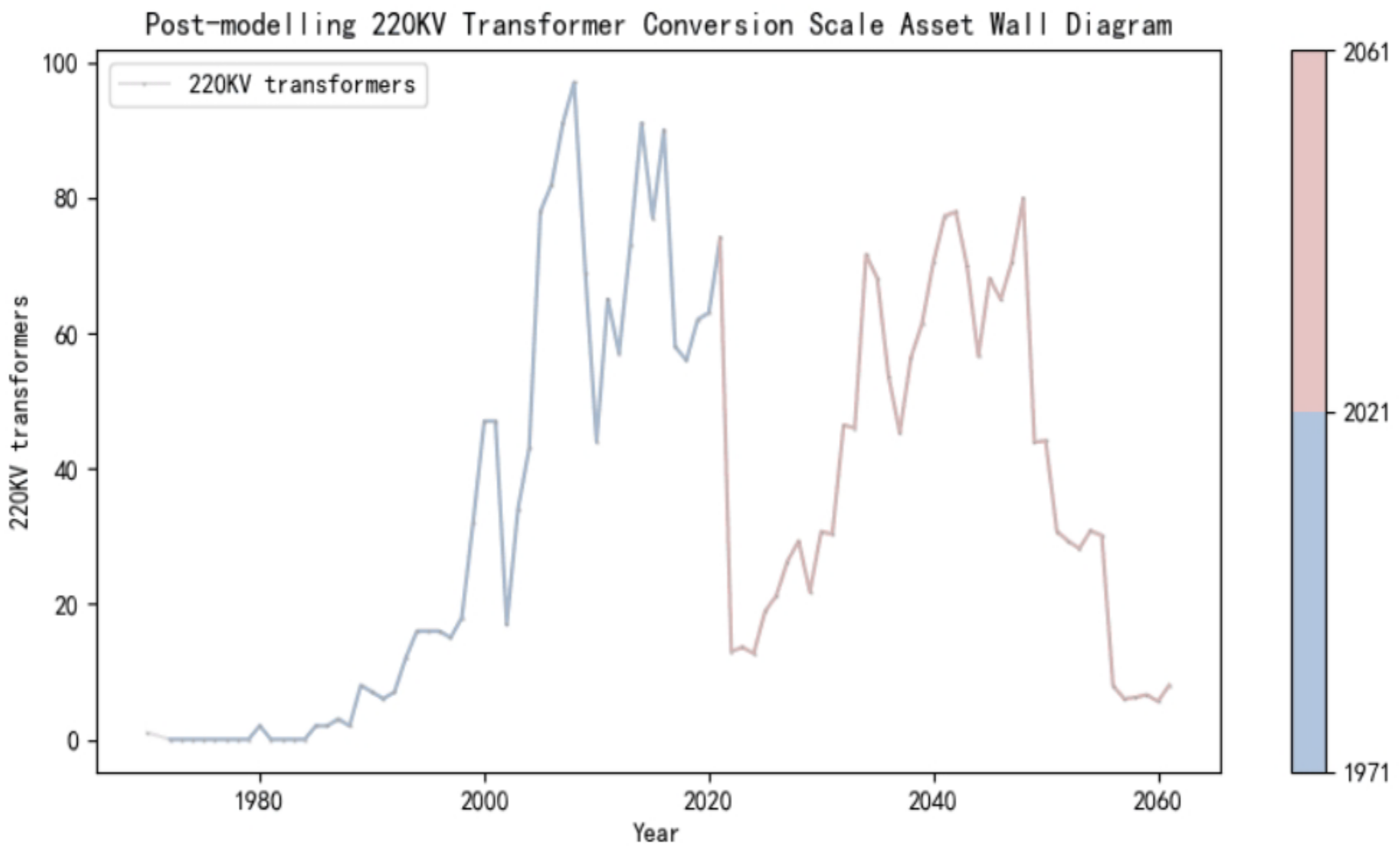
According to the above process and simulation rules, the future device decommissioning scale of 220 KV transformers is obtained (Figure 9).

For the analysis of Figure 9, the peak periods of in-operation equipment for 220 KV transformers were 2007, 2014, and 2020, and the peak periods of retirement after conducting MC were 2035, 2042, and 2048, which roughly correspond to the peak periods of equipment. Comparing the peaks, it could be seen that the peak of the equipment curve after MC was significantly lower than the peak of the equipment in operation, and the effect of the model was very significant.

Similarly, the same steps can be used to obtain the future decommissioning scale of the 110 KV circuit breakers (Figure 10).

According to Figure 10, the equipment in operation would be retrofitted from 2022 to 2061. The scale of the conversion was very similar to the fluctuation of the previous equipment input scale, but the peak of the future conversion scale was obviously reduced, which had a better effect of “cutting the peaks and filling the valleys” and again verified the feasibility of the empirical simulation.

3.4. Comparison between AW and WMCAW

This paragraph used AW to forecast the scale of equipment replacement in order to compare the results with those obtained by WMCAW and to illustrate the applicability of WMCAW. Because AW measured its value scale directly in the application, in this paper for a better comparison, we directly forecasted the number of equipment replacements using AW, and prices we considered separately in the Section 3.5 Price Forecast. Based on actual measurements, it could be seen that the average service life of 220 KV transformers was 26 years and the life was used as the basis for the AW panning. At the same time, the equipment that exceeded the average service life but was still operating was taken into direct retirement in 2022, which yielded Figure 11.

According to Figure 11, it could be seen that the graphs obtained using AW were generally consistent with the historical commissioning trends. For example, the peak of 220 KV transformer commissioning was reached in 2011, which, according to AW, corresponded to the peak of equipment replacement in 2037. The result was obvious because the average service life of the equipment was 26 years and the method was a simple mechanical leveling of the historical scale.

Compared to Figure 9, it is obvious that the forecast curve trend of the WMCAW method after 2022 was more moderate than that of AW. In order to better illustrate the difference between the data, we compared six indicators (sources of data: AW for 2022–2047, WMCAW for 2022–2061) and obtained

Table 2. Comparison chart of WMCAW and AW data indicators for 220 KV transformers.

	AVG	MAX	MIN	SD	SKEW	KURT
WMCAW	11.225	25.6	1.1	7.584321	0.329105	−1.23339
AW	17.26923	34	2	8.291237	−0.12013	−0.5347

.

According to the table, we see that the AVG (WMCAW) was smaller than AW, the MAX (WMCAW) was smaller than AW, and the MIN (WMCAW) was bigger than AW, which fully showed that using MC could not only extend part of retired life of equipment reasonably but also could effectively peak “cut”, presenting the equipment retired scale in a more stable state. Furthermore, the smaller the SD, the smaller the discrete degree of the data set, and the more stable the device data. SKEW was an indicator to measure the central tendency of equipment data. The data of AW was left-skewed, while the data of WMCAW was right-skewed. KURT is an index to measure the flatness of the data peak. The smaller the value, the more smooth the peak tended to be. Obviously, the former had a flatter peak.

Similarly, according to the calculation, the average service life of a 110 KV circuit breaker was 32 years. The 110 KV circuit breakers were analyzed by the same steps, and Figure 12 was obtained.

According to Figure 12, the trend of AW was still consistent with the historical trend. By comparing the figures of the two models, we could find that the modification effect of 110 KV circuit breakers using WMCAW is better than that of 220 KV transformers, and their peak period was weakened more obviously, which could also be seen in

Table 3. Comparison chart of WMCAW and AW data indicators for 110 KV circuit breakers.

	AVG	MAX	MIN	SD	SKEW	KURT
WMCAW	70.95	241.1	2.5	60.50783	1.069664	0.394752476
AW	88.6875	429	0	99.08661	1.728404	3.39945569

.

According to the indicators: MAX: WMCAW > AW, MIN: WMCAW < AW, AVG: WMCAW < AW, SD: WMCAW < AW. The conclusion is that WMCAW was more stable could be fully obtained. The SKEW of AW was larger, indicating that the data were more left-skewed, while the KURT of AW was significantly larger than that of WMCAW, which fully proved that the data peak of the latter is larger.

According to the empirical results, we concluded that the prediction scale of MWCAW was more stable than AW, so we believed that the model proposed in this paper was effective. Stable prediction results are very important for the replacement scale of energy enterprises. Weakening the peak period of the equipment replacement scale can ensure the operation of enterprises to carry out retirement in a more orderly manner. The model considers the randomness of equipment decommissioning, and its prediction results are more scientific than AW. Moreover, when considering the price, a stable replacement scale is conducive to the stability of the capital chain and reduces the probability of insufficient funds in the peak period of equipment replacement.

3.5. Price Forecast

Firstly, the price of 220 KV transformers is forecasted, and since there are many missing values in price before 1990, the price data from 1990 to 2021 were selected and decomposed by VMD, a total of 11 IMFs are obtained, and the decomposition effect is shown in Figure 13.

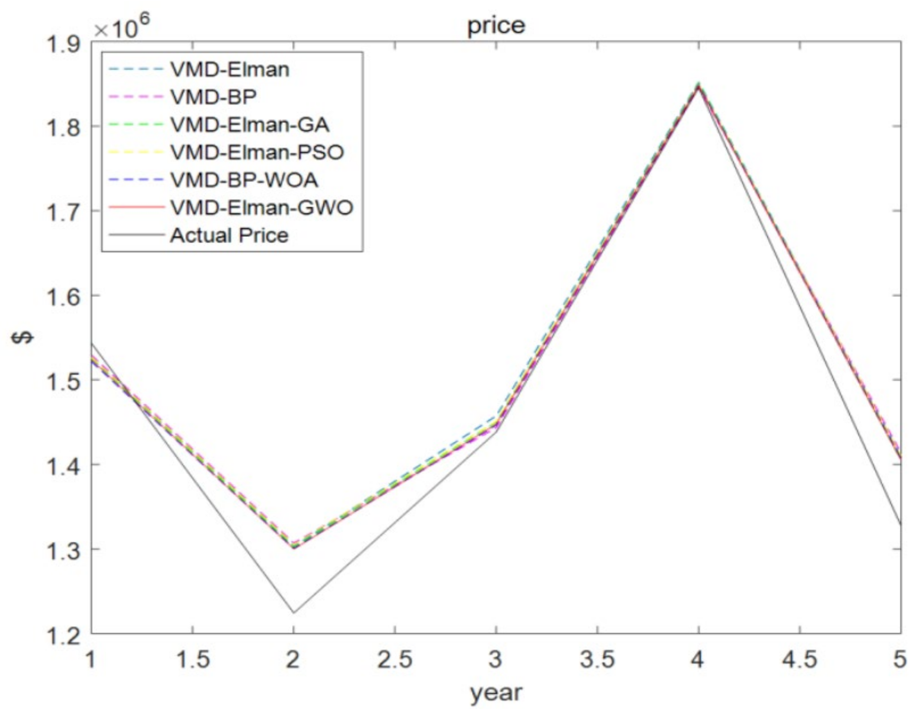
In this article, the BP and Elman neural networks are used for prediction based on VMD decomposition, and various optimization algorithms (e.g., PSO, WOA, GA) are used to optimize the five-year 220 KV transformer price. A graph of the fitting effect of each optimization algorithm for 220 KV transformer prices was obtained (shown in Figure 14).

According to Figure 14, it can be observed that the fitting effects of various types of decomposition optimization algorithms were similar and all were relatively good. In order to verify the differences in fitting effects between various types of optimization algorithms, the errors of various models were compared by comparing the results as shown in

Table 4. Error diagram of each model for 220 KV transformer price forecast.

	MAE	MAPE	RMSE
VMD-Elman-GA	37,998.09	2.888643	50,164.97864
VMD-Elman-GWO	36,943.02	2.815927	49,442.98488
VMD-Elman-PSO	39,317.38	2.997736	52,565.24256
VMD-Elman	40,630.82	3.074133	52,045.52512
VMD-BP	37,745.58	2.909011	53,720.5302
VMD-BP-WOA	37,632.3	2.863269	50,155.61527

.

By comparing the three error indicators of MAE, MAPE, and RMSE to various models, the model with the smallest MAE indicator was the VMD-Elman-GWO optimization algorithm with a value of 36,943.02; the model with the smallest MAPE indicator was the VMD-Elman-GWO optimization algorithm with the value of 2.815927; similarly, the RMSE indicator could be obtained as the most model was also the VMD-Elman-GWO optimization algorithm. In summary, we choose the VMD-Elman-GWO optimization algorithm model to forecast the price of 220 KV transformers in the next five years. The forecast results are shown in

Table 5. Price forecast for 220 KV transformers for the next five years.

Year	Price
2022	1,572,423.065
2023	1,291,444.871
2024	1,385,758.873
2025	1,257,645.102
2026	1,337,847.378

.

According to Table 5, we obtained the 220 KV transformer prices for the next five years. According to the forecast, the average unit price of this equipment reaches the highest value of $1,572,423.065 in 2022; the lowest was 2025 with a value of $1,257,645.102; the overall price change was fluctuating, and there was no significant upward or downward trend.

Similarly, forecasting the price of 110 KV circuit breakers, we can decompose the price of 110 KV circuit breakers into 11 IMFs using VMD, as shown in Figure 15, below. since 110 KV circuit breakers started to be put into operation on a large scale in 1994, we chose the average price data of 110 KV circuit breakers from 1994 to 2021 for our analysis.

Similarly, the BP and Elman neural networks were used for prediction on the basis of VMD decomposition, and various optimization algorithm models were used to optimize the five-year 110 KV circuit breaker prices, and the fitting effect diagram of each optimization algorithm of the price of 110 KV circuit breaker was obtained, as shown in Figure 16.

According to Figure 16, it could be found that the fitting effect of VMD-Elman-GWO was slightly better than other optimization algorithms. In order to better verify the difference in fitting effect between various optimization algorithms, similar to the treatment of 220 KV transformers, we selected three indicators, MAE, MAPE, and RMSE, to compare the errors of each combination model, and the following

Table 6. Error table for each model of 110 KV circuit breaker price forecast.

	MAE	MAPE	RMSE
VMD-Elman-GA	995.1635	4.4757	1004.6
VMD-Elman-GWO	930.7674	4.1487	980.5712
VMD-Elman-PSO	950.0764	4.2650	1023.983
VMD-Elman	935.6410	4.0872	1051.779
VMD-BP	956.6896	4.2572	979.0357
VMD-BP-WOA	960.9707	4.4006	989.2229

was obtained.

According to the results in Table 6, the MAE of the VMD-Elman-GWO optimization algorithm was the smallest among all optimization models, and the MAPE and RMSE values were ranked fifth, so the VMD-Elman-GWO optimization algorithm is the most suitable 110 KV circuit breaker price prediction model.

So, using the VMD-Elman-GWO algorithm to forecast the price of 110 KV circuit breakers for the next five years, we obtained

Table 7. Price forecast for 110 KV circuit breakers for the next five years.

Year	Price
2022	16,483.81601
2023	24,086.63351
2024	19,899.29797
2025	24,681.17964
2026	27,945.10401

.

According to Table 7, the price of 110 KV circuit breakers is the lowest in 2022 with a value of $16,483.81601 and reaches a peak of $27,945.10401 in 2026; the overall analysis of the data for the next five years shows a clear upward trend in the overall price, with the price in 2026 being almost 1.7 times higher than that in 2022.

3.6. Asset Wall Integration

Based on Section 3.3 and Section 3.4, we aggregate the obtained quantitative asset wall model and price forecast data to obtain an improved value asset wall model.

A modified wall model was used to forecast the size of the value of 220 KV transformers for the next five years of retirement. Figure 15 shows the results of the data selected for 2010–2021 and the integration of data for 2022–2026.

According to Figure 17, there was a clear downward trend in the value scale of technological improvements from 2022 to 2026 compared to the value scale of the last decade, mainly because the technological improvements in the next five years are targeted at equipment in operation around 2000, since the volume scale has increased significantly in recent years, and the actual capital costs incurred in the last decade have also produced a clear upward trend compared to 2000–2010. The trend is that the improved wall model will reduce the number of pieces of equipment decommissioned during this peak period and reduce the capital risk.

Similarly, the volume wall and price forecast data for 110 KV circuit breakers were aggregated to obtain the value scale wall, i.e., Figure 18.

Figure 18 shows a very similar situation to Figure 17, due to the significant increase in 110 KV circuit breakers in the last ten years, while 2022–2026 reflects the first twenty years of input equipment decommissioning, so even though the price of transformers shows a rapid upward trend in the next five years, the scale of retirement funding for this equipment in 2022–2026 is still significantly reduced compared to the scale of the last ten years.

3.7. Empirical Conclusions and Research Outcomes

In this work, the decommissioning rate curve of the equipment was corrected by the Weibull distribution to ensure that the curve fitted the decommissioning pattern of the equipment and that its overall fit was good in Section 3.1. In Section 3.2, we used AW to draw an asset wall based on the actual number of equipment in operation in each year of input, in preparation for the subsequent MC. In Section 3.3, MC was performed based on the decommissioning rate curve and the asset wall of in-service equipment to obtain the predicted number of in-service equipment replacements for each future year. The results were collapsed into the asset wall of Section 3.3 and carried forward by year. In Section 3.4, we compared the difference between the predicted asset wall and the actual asset wall and found that the average number of decommissions in each year of the asset wall obtained with WMCAW was less than that of AW. At the same time, the former effectively weakened the peak of equipment replacement, which can effectively ensure the stability of the capital chain and prevented underfunding due to potential equipment retirement peaks, proving the need for this paper’s research. In Section 3.5, firstly the noise of the equipment price curve was reduced by VMD, and then each neural network model was compared to obtain the best model for predicting equipment prices (VMD-Elman-GWO) for equipment prices over the next five years, the forecast errors were within acceptable limits, and we considered the forecast prices to be meaningful. The projected equipment quantities and prices were integrated in Section 3.6 to form the final asset wall of equipment values. A comparison of the asset wall for 2022–2026 with that for 2010–2021 clearly showed that the replacement of equipment over the next five years was relatively small, mainly due to the fact that less equipment remained retired over the next five years. At the same time, the years 2022–2026 showed a clear upward trend, mainly due to the fact that overall equipment prices showed a clear upward trend, and it was foreseeable that there will still be significant financial pressure in the future.

In summary, we believe that this study is necessary to provide significant value to the development of energy companies in both equipment management and sustainable development through this methodology.

The main outcomes of the paper are summarized as follows:

• WMCAW can help energy enterprises to be fully prepared to deal with financial risk when they face a possible peak in equipment replacement in the future. Meanwhile, the model has the effect of “cutting the peak and filling the valley”. Compared to the AW model, the WMCAW model can effectively reduce the number of equipment replacement peaks during the same period, providing for maintaining the stability of the capital chain and for the safe, efficient, and stable operations of energy enterprises.
• WMCAW offers reasonable advice on how to identify equipment replacement risk mitigation measures, propose an optimal approach to corporate investment strategy, and achieve precise investment in equipment replacement.

4. Policy Implication and Future Work

Before the 21st century, when energy companies were not very large, there was still a single goal-based approach to work, i.e., the important aim was to ensure the stable and safe operation of equipment and to satisfy the need for the repair and replacement of equipment as far as possible, without much consideration of economic factors. However, with the rapid growth in the size of energy companies over the last 20 years, this model is no longer appropriate for the management of equipment in energy companies.

The predictive research in the paper provides significant value in improving the working pattern of energy companies from a single to a multi-objective type. Energy companies can calculate the actual number of commissioned equipment and the decommissioning rate for each year, and get the number of equipment to be replaced in each future year according to the model. Replacing equipment and preparing funds according to this predicted number will not only still maintain stable equipment operation, but also take into account economic factors, weaken potential future equipment replacement peaks, taking into account economic factors, smoothing the amount of capital invested by energy companies each year, and providing a reference for companies to prepare equipment replacement capital in advance, thus better enabling the sustainability of energy equipment.

In the future, the shortcomings in the WMCAW model will be further studied. The model is applicable to a large amount of equipment put into operation with a long service life. For the others, the model’s predictions will be not accurate because of errors in the simulation probabilities, so we need to pay attention to some of the work in forecasting the scale of the replacement of these devices. Furthermore, for equipment in operation that has exceeded the maximum life in the decommissioned equipment sample, we selected its retirement for the current year. However, whether energy companies can afford the huge costs involved in using WMCAW is a question that needs to be explored, as it is important to ensure the scientific validity of the data while taking into account as many economic and human factors as possible in practice.