Modal Identification of Low-Frequency Oscillations in Power Systems Based on Improved Variational Modal Decomposition and Sparse Time-Domain Method

Abstract

Power systems have an increasing demand for operational condition monitoring and safety control aspects. Low-frequency oscillation mode identification is one of the keys to maintain the safe and stable operation of power systems. To address the problems of low accuracy and poor anti-interference of the current low-frequency oscillation mode identification method for power systems, a low-frequency oscillation mode feature identification method combining the adaptive variational modal decomposition and sparse time-domain method is proposed. Firstly, the grey wolf optimization algorithm (GWO) is used to find the optimal number of eigenmodes and penalty factor parameters of the variational modal decomposition (VMD). And the improved method (GWVMD) is used to decompose the measured signal with low-frequency oscillations and then reconstruct the signal to achieve a noise reduction. Next, the processed signal is used as a new input for the identification of the oscillation modes and their parameters using the sparse time-domain method (STD). Finally, the effectiveness of the method is verified by the actual low-frequency oscillation signal identification in the Hengshan power plant and numerical signal simulation experiments. The results show that the proposed method outperforms the conventional methods such as Prony, ITD, and HHT in terms of modal discrimination. Meanwhile, the overall reduction in the frequency error is 34, 44, and 21%, and the overall reduction in the damping error is 37, 41, and 18%, compared with the recently proposed methods such as the EFEMD-HT, RDT-ERA, and TLS-ESPRIT. The effectiveness of the methods in suppressing the modal confusion and noise immunity is demonstrated.

1. Introduction

With the continuous expansion of the scale of the power network, the close connection between the power grids in various regions and the dramatic increase in the demand for electrical energy have led to some oscillation accidents in the power system from time to time [1]. Among these, the risk of ultra-low-frequency oscillation and low-frequency oscillation of power-system-producing units is rising, particularly in the power network dominated by hydroelectric units [2,3]. If such low-frequency oscillation events are allowed to progress without prompt treatment, the risks they pose will definitely interfere with the regular operation of the entire generating unit [4]. The early and precise identification of the oscillation modes and associated systemic factors is the key to managing low-frequency oscillations in a power system [5]. In the actual operating environment, it is challenging to clearly distinguish the unit’s modal properties from the background noise. For ensuring the secure and stable functioning of thermal power-generating units, the investigation of the low-frequency oscillation mode identification is crucial [6,7].

When the power system is perturbed to varying degrees by load fluctuations, equipment failures, etc., electrical quantities such as the system power angle, power, and voltage oscillate to varying degrees. This phenomenon is known as low-frequency oscillation, and it refers to the relative oscillation between the rotors of synchronously running generators. This oscillation typically occurs between 0.2 and 2.5 Hz. Low-frequency oscillation can be split into two categories, the regional oscillation mode and local oscillation mode, depending on the range that it involves. The interconnection inter-regional contact line power oscillation is the regional oscillation mode. Through the contact line, the oscillation power is transmitted throughout the entire system. The system is more negatively impacted. The oscillation between units in the plant station is referred to as the local oscillation mode. It mostly has an impact on the power exchange in the vicinity of the oscillation. The primary mechanical sources of the low-frequency oscillations at the moment include negative damping, forced oscillation, parametric resonance, and nonlinear mechanisms [8]. At this stage, the methods of the low-frequency oscillation problems can be mainly divided into two types of methods, such as the theoretical analysis methods based on the system structure and model parameters [9] and the signal analysis methods based on a dynamic simulation or real measurement data [10].

The theoretical analysis methods based on the system structure and model parameters mainly include an electrical torque analysis, eigenvalue analysis, and a regular shape and time-domain analysis. In the literature [11], the electrical torque method is applied to analyze the effects of the PV penetration rate, PV plant location, and controller speed loop and power angle loop feedback PID gain on the electromechanical oscillation effect of a PV suppression system in electromechanical time scale, respectively. In the literature [12], an eigenvalue analysis method is used to analyze the effects of three factors, namely the grid strength, power level, and control parameters, on low-frequency oscillations. The oscillation suppression measures of changing the controller parameters and adding additional controllers are proposed. The stability analysis problem of the low-frequency oscillation at the DC side is solved. In the literature [13], the second-order approximate analytical solution of the state equation of the power system is derived based on the regular shape transformation of the nonlinear vector field. A nonlinear index is proposed to measure the magnitude of the nonlinearity of the power system, and the nonlinear correlation between the low-frequency oscillation modes and the influence on the dynamic characteristics of the power system are revealed. The time-domain simulation method can consider the nonlinear characteristics of the system without the limitation of the system size [14]. However, the identification results are easily affected by the location and class of disturbances and require longer simulation time as the system size increases.

The signal analysis methods based on a dynamic simulation or real data mainly include Prony, Fourier transform, HHT, and deep learning methods. A Prony analysis [15] uses a linear superposition of a set of exponential terms to fit the isometric sampled data. The analysis can be used to obtain information such as the signal amplitude, initial phase, damping factor, and oscillation frequency from it. However, the Prony method has a low accuracy when dealing with non-stationary signals due to its own fitting nature and easy noise effects [16]. The Fourier transform method is less effective in the identification of time-varying or non-stationary modes [17]. Without the further processing of the signal frequency domain, the damping characteristics of the signal cannot be obtained by direct information, and thus it is difficult to distinguish such modal information. The HHT methods [18] can effectively identify non-smooth signals. The HHT methods are mainly the empirical mode decomposition (EMD) [19] and Hilbert transform, respectively. The EMD decomposes the original signal into a multiple intrinsic mode function (IMF), and then the Hilbert transform is used to identify the modal parameters. However, the EMD is prone to problems such as modal mixing in the signal decomposition process, which leads to the poor overall identification of the HHT method. The literature [20] proposes a deep learning-based algorithm for determining the order of multi-order LFO signals. A deep belief network (DBN) consisting of a Restricted Boltzmann Machine (RBM) superposition is chosen as the algorithm model, and the recognition of the low-frequency oscillation signal order is achieved with the help of the DBM training algorithm. In the literature [21], a singular value decomposition, group search algorithm, and deep belief network are also used to solve the low-frequency oscillation mode identification problem. Compared to the traditional low-frequency oscillation modal analysis method, it also has a certain effect on noise immunity [22], but the method ignores the modal time-varying and non-smooth characteristics of low-frequency oscillation [23].

Most of the traditional low-frequency oscillation discrimination methods can only achieve the discrimination of single-channel parameters and cannot handle multiple signals at the same time. The random decrement method (ITD) [24] is a common method to achieve the multi-channel discrimination of parameters. However, the recognition accuracy of this method is low when processing low signal-to-noise ratio signals. The sparse time-domain method (STD) is a commonly used method for the extraction of low-frequency oscillation mode parameters [25]. This algorithm is less computationally intensive and more efficient in operation during the operation of the matrix. The literature [26] uses the sparse time-domain method (STD) to extract the oscillation mode parameters. However, the lack of a certain signal preprocessing link leads to a low accuracy of the parameters identified by the algorithm in the case of a low signal-to-noise ratio. The literature [27] uses wavelet thresholding for signal denoising. However, there are problems of a difficult selection of the threshold and wavelet ridges and defects in the threshold function itself, which lead to the distortion of the processed signal waveform and reduce the accuracy of the identification of key oscillation mode parameters. Variational mode decomposition (VMD) is a new time–frequency analysis method with the advantages of no smooth signal assumptions and the adaptive decomposition of low-frequency oscillation signals. The literature [28] uses the VMD method to extract the main trends of the partial discharge characteristic parameters, excluding the influence of the noisy oscillatory components on the real-time evaluation. The effectiveness of the VMD method for signal denoising is also demonstrated in the literature [29]. However, the problem of taking the number of eigenmodes and penalty factors in the VMD method is still one of the main difficulties at present.

In this paper, we propose a method to identify the low-frequency oscillation mode features of a unit by combining an improved variational modal decomposition with a sparse time-domain method. First, we propose a novel variational modal decomposition method (GWVMD). We use the gray wolf optimization algorithm (GWO) to determine the optimal eigenmodes number and penalty factor values for the VMD. Then, we use the improved variational modal decomposition method to decompose and reconstruct the measured signal with low-frequency oscillations to filter out the noise in the signal and improve the modal parameter identification performance of the sparse time-domain method. Finally, we use the sparse time-domain (STD) method for the identification of the modes and their parameters. The proposed method solves the problems of low accuracy and poor anti-interference in the low-frequency oscillation modal discrimination of power systems. The effectiveness of the proposed method is verified by the real low-frequency oscillation signal identification experiments of the Hengshan power plant units.

The main contributions of this research are as follows:

(1)

We propose a method for the modal feature identification of low-frequency oscillations of a unit by combining the improved variational modal decomposition with the sparse time-domain method. The method improves the accuracy and anti-interference in the modal discrimination of low-frequency oscillation signals in power systems.

(2)

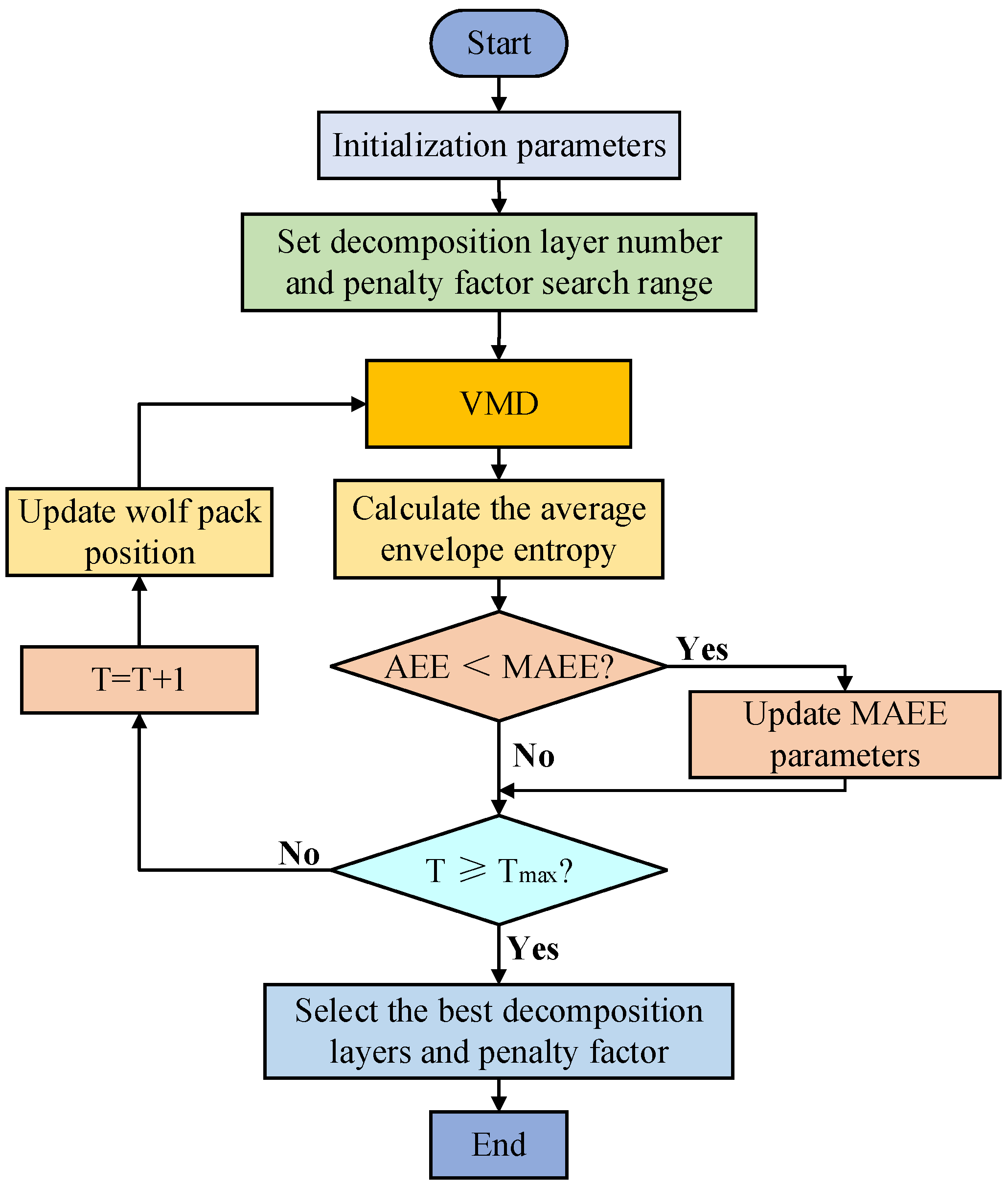
We use the grey wolf optimization algorithm (GWO) to find the optimal number of eigenmodes and penalty factors for the VMD. The noise in the signal is also filtered out using the improved variational modal decomposition (GWVMD).

(3)

We use the sparse time-domain method to accurately identify the modal parameters in the noise-reduced low-frequency oscillation signal and solve the multi-channel identification performance of the low-frequency oscillation identification method.

(4)

Through the signal identification experiments in the Hengshan power plant, it can be concluded that the GWVMD-STD method has an overall reduction of 34, 44, and 21% in the frequency error and 37, 41, and 18% in the damping error compared to the EFEMD-HT, RDT-ERA, and TLS-ESPRIT methods.

The rest of this paper is organized as follows: Section 2 and Section 3 introduce the basic principles of the variational modal decomposition and the sparse time-domain method. Section 4 presents the basic steps for improving the variational modal decomposition method and the overall modal identification method, and the evaluation indexes for subsequent experiments. In Section 5, a comparison experiment of the low-frequency oscillation identification of the Hengshan power plant and a numerical simulation are conducted to verify the effectiveness and superior performance of the proposed model. Finally, the identification method and experimental results are discussed and analyzed, and the conclusions of the research are given.

2. Variational Modal Decomposition

Variational modal decomposition (VMD) is a new signal adaptive processing method. The adaptive decomposition of the signal is achieved by continuously and iteratively updating the frequency center and bandwidth of each oscillation mode. Compared with the empirical modal decomposition (EMD) method, it has a better performance and higher operational efficiency in anti-noise and non-smooth signal processing.

The variational modal decomposition decomposes the original signal into multiple modal functions with different center frequencies by an adaptive filter bank. Set $f(x)$ as the original signal, ${\omega }_k$ as the center frequency, and $u_k$ as the mode function. To obtain the modal components with different bandwidth frequencies, a Hilbert transform is usually applied to each modal function $u_k$ to obtain the marginal spectrum.

$$h_k(t)=\left(\delta (t)+\frac{\mathrm{j}}{\pi t}\right)\times u_k(t)$$

(1)

where $\delta (t)$ is the Dirichlet function; $k$ is the number of preset modal components; $h_k(t)$ is the marginal spectrum of each mode. The center frequency of the resolved signal of each mode is predicted, and the spectrum of each mode is modulated to the corresponding fundamental frequency band.

$${\eta }_k(t)=\left(\delta (t)+\frac{\mathrm{j}}{\pi t}\right)\times u_k(t)*{\mathrm{e}}^{-\mathrm{j}{\omega }_{k}t}$$

(2)

where ${\eta }_k(t)$ is the fundamental frequency band of each mode; * is the convolution sign. By calculating the signal gradient’s squared parametrization, the signal bandwidth of each mode is determined. The below is a possible formulation of the constrained variational problem.

$$\{\begin{array}{l}{\min }_{\left\{u_k\right\},\left\{{\omega }_k\right\}}\left\{{\displaystyle \sum _k{\Vert {\partial }_t\left[\left(\delta (t)+\frac{\mathrm{j}}{\pi t}\right)\times u_k(t)\right]{\mathrm{e}}^{-\mathrm{j}{\omega }_{k}t}\Vert }_2^2}\right\}\hfill \\ \mathrm{s}.\mathrm{t}.\hspace{1em}{\displaystyle \sum _k{u}_k}=f(t)\hfill \end{array}$$

(3)

where $\left\{u_k\right\}=\{u_1,\dots ,u_k\}$ is the $k$ modal components obtained by decomposition; $\left\{{\omega }_k\right\}=\{{\omega }_1,\dots ,{\omega }_k\}$ is the frequency center of each component. By introducing the penalty factor and the Lagrangian operator, the augmented Lagrangian formula can be obtained as

$$L\left(\left\{u_k\right\},\left\{{\omega }_k\right\},\lambda \right)=\alpha {\displaystyle \sum _k{\Vert {\partial }_t\left[\left(\delta (t)+\frac{\mathrm{j}}{\pi t}\right)\times u_k(t)\right]{\mathrm{e}}^{-\mathrm{j}{\omega }_{k}t}\Vert }_2^2}+{\Vert f(t)-{\displaystyle \sum _k{u}_k}(t)\Vert }_2^2+\left[\lambda (t),f(t)-{\displaystyle \sum _k{u}_k}(t)\right]$$

(4)

where $\alpha$ is the penalty factor; $\lambda (t)$ is the Lagrangian multiplicative operator.

The saddle point of the augmented Lagrangian expression is sought by alternately updating $u_k^{n+1}$, ${\omega }_k^{n+1}$, and ${\lambda }_k^{n+1}$, thus decomposing $f$ into $k$ narrowband IMF components. The computational equation is given by

$${\widehat{u}}_k^{n+1}(\omega )=\frac{\widehat{f}(\omega )-{\displaystyle \sum _{i\ne k}{\widehat{u}}_i}(\omega )+\frac{\widehat{\lambda }(\omega )}{2}}{1+2\alpha {\left(\omega -{\omega }_k\right)}^2}$$

(5)

$${\omega }_k^{n+1}=\frac{{\displaystyle {\int }_0^{\infty }\omega }{\left|{\widehat{u}}_k(\omega )\right|}^{2}d\omega }{{\displaystyle {\int }_0^{\infty }{\left|{\widehat{u}}_k(\omega )\right|}^2}d\omega }$$

(6)

$${\widehat{\lambda }}^{n+1}(\omega )={\widehat{\lambda }}^n(\omega )+\tau \left[\widehat{f}(\omega )-{\displaystyle \sum _k{\widehat{u}}_k^{n+1}}\right]$$

(7)

where the Fourier transform forms of $u_k^{n+1}$, ${\omega }_k^{n+1}$, and ${\lambda }_k^{n+1}$ are ${\widehat{u}}_k^{n+1}(\omega )$, ${\omega }_k^{n+1}$, and ${\widehat{\lambda }}^{n+1}(\omega )$, respectively.

3. Sparse Time-Domain Method

In the presence of an oscillating signal $x(t)$, setting the eigenvalue of the oscillation mode to ${\lambda }_i$, the angular frequency to ${\omega }_i$, the damping ratio to ${\xi }_i$, and the oscillation coefficient to $p_i$, we can obtain the signal representation in the form of a linear combination of complex exponential functions.

$$x(t)={\displaystyle \sum _{i=1}^m{p}_i}{\mathrm{e}}^{{\lambda }_{i}t}={\displaystyle \sum _{i=1}^m{p}_i}{\mathrm{e}}^{\left(-{\xi }_i{\omega }_i+\mathrm{j}{\omega }_i\sqrt{1-{\xi }_i^2}\right)t}$$

(8)

where $n$ is the system order, $m=2n$. We sample the observation points in the signal to derive the response matrix.

$$\mathsf{\Phi }=\left[\begin{array}{cccc}{x}_1\left(t_1\right)& x_1\left(t_2\right)& \cdots & x_1\left(t_N\right)\\ x_2\left(t_1\right)& x_2\left(t_2\right)& \cdots & x_2\left(t_N\right)\\ ⋮& ⋮& & ⋮\\ x_r\left(t_1\right)& x_r\left(t_2\right)& \cdots & x_r\left(t_N\right)\end{array}\right]$$

(9)

where $r$ is the number of observation points of the system and $\mathsf{\Phi }$ is the constructed response matrix. The fusion of Equations (8) and (9) leads to:

$$\mathsf{\Phi }=\left[\begin{array}{cccc}{p}_{11}& p_{12}& \cdots & p_{1m}\\ p_{21}& p_{22}& \cdots & p_{2m}\\ ⋮& ⋮& & ⋮\\ p_{r1}& p_{r2}& \cdots & p_{rm}\end{array}\right]\left[\begin{array}{cccc}{\mathrm{e}}^{{\lambda }_1{t}_1}& {\mathrm{e}}^{{\lambda }_1{t}_2}& \cdots & {\mathrm{e}}^{{\lambda }_1{t}_1}\\ {\mathrm{e}}^{{\lambda }_2{t}_1}& {\mathrm{e}}^{{\lambda }_2{t}_2}& \cdots & {\mathrm{e}}^{{\lambda }_2{t}_N}\\ ⋮& ⋮& & ⋮\\ {\mathrm{e}}^{{\lambda }_m{t}_1}& {\mathrm{e}}^{{\lambda }_m{t}_2}& \cdots & {\mathrm{e}}^{{\lambda }_m{t}_N}\end{array}\right]$$

(10)

To calculate the unknown elements in the matrix, calculate the response matrix $\widehat{\mathsf{\Phi }}$ after a delay of $\Delta t$.

$$x\left(t_{k+1}\right)=x\left(t_k+\Delta t\right)={\displaystyle \sum _{i=1}^m{p}_i}{\mathrm{e}}^{{\lambda }_i\left(t_k+\Delta t\right)}$$

(11)

$$\widehat{\mathsf{\Phi }}=\left[\begin{array}{cccc}{x}_1\left(t_2\right)& x_1\left(t_3\right)& \cdots & x_1\left(t_{N+1}\right)\\ x_2\left(t_2\right)& x_2\left(t_3\right)& \cdots & x_2\left(t_{N+1}\right)\\ ⋮& ⋮& & ⋮\\ x_r\left(t_2\right)& x_r\left(t_3\right)& \cdots & x_r\left(t_{N+1}\right)\end{array}\right]$$

(12)

Because $B=\widehat{\mathsf{\Phi }}/\mathsf{\Phi }$, we can calculate the individual elements $b_i$ in matrix $B$.

$$B=\left[\begin{array}{cccccc}0& 0& 0& \cdots & 0& b_1\\ 1& 0& 0& \cdots & 0& b_2\\ 0& 1& 0& \cdots & 0& b_3\\ ⋮& ⋮& ⋮& & ⋮& ⋮\\ 0& 0& 0& \cdots & 1& b_N\end{array}\right]$$

(13)

After obtaining matrix $B$, we can calculate the frequency and damping ratio of the signal as shown in the following Equations (14) and (15).

$$f_i=\frac{\ln {\lambda }_i}{2\pi \Delta t}$$

(14)

$${\xi }_i=\frac{1}{\sqrt{1+{\left(\mathrm{Im}\left(V_i\right)/\mathrm{Re}\left(V_i\right)\right)}^2}}$$

(15)

where $f_i$ is the frequency, ${\xi }_i$ is the damping ratio, and the eigenvalue of the matrix is ${\tilde{\lambda }}_i={\mathrm{e}}^{{\lambda }_i\Delta t}$. We can analyze the reconstructed signal after noise reduction using the sparse time-domain method to identify the frequencies and damping ratios in each mode.

4. Low-Frequency Oscillation Mode Identification Based on Improved VMD and STD

4.1. Improvement in Variational Modal Decomposition

To solve the problem that the eigenmodes number and penalty factor of the variational modal decomposition are difficult to determine, we use the gray wolf optimization algorithm (GWO) to improve the VMD and find the optimal solution of the two parameters. The gray wolf optimization (GWO) algorithm has the advantages of fast convergence, high optimization efficiency, and short running time compared to other metaheuristic swarm intelligence algorithms. However, the algorithm suffers from premature convergence and the tendency to fall into local optima [30].

The basic principle of gray wolf optimization (GWO) is that the wolves are arranged in descending order according to the fitness function and are classified into four classes, namely $a_1$, $b_1$, $c_1$, and $d_1$. The optimal solution is found by updating the values through continuous iterations and finally completing the search for the optimal solution, in which the optimal solution of the objective function is determined by $a_1$, $b_1$, and $c_1$ in the solution process and executed by $d_1$ to obtain the optimal solution. The GWO for position updating is as follows:

$$x(t+1)=\frac{{\displaystyle \sum _{i=1}^3{x}_i}}{3}$$

(16)

$$\{\begin{array}{l}{x}_1=x_{a_1}-A_1\cdot D_{a_1}\\ x_2=x_{b_1}-A_2\cdot D_{b_1}\\ x_3=x_{c_1}-A_3\cdot D_{c_1}\end{array}$$

(17)

$$\{\begin{array}{l}{D}_{a_1}=\left|C_1\cdot x_{a_1}-X\right|\\ D_{b_1}=\left|C_2\cdot x_{b_1}-X\right|\\ D_{c_1}=\left|C_3\cdot x_{c_1}-X\right|\end{array}$$

(18)

where $X$ denotes the current optimal solution; $C_1$ and $A_1$, $C_2$ and $A_2$, $C_3$ and $A_3$ are the coefficient vectors of wolf packs $a_1$, $b_1$, and $c_1$, respectively; $x_{a_1}$, $x_{b_1}$, and $x_{c_1}$ are the current position vectors of wolf packs $a_1$, $b_1$, and $c_1$, respectively; $t$ denotes the number of iterations. We choose MAEE as the fitness function to find the optimum for the relevant parameters.

$$\langle \widehat{k},\widehat{\alpha }\rangle =\underset{(k,\alpha )}{\arg \min }\left\{\frac{1}{\widehat{k}}{\displaystyle \sum _{i=1}^k{H}_{\mathrm{en}}}(i)\right\}$$

(19)

$$p_j=\frac{a(j)}{{\displaystyle \sum _{j=1}^{N}a}(j)}$$

(20)

$$H_{\mathrm{en}}=-{\displaystyle \sum _{j=1}^N{p}_j}\log \left(p_j\right)$$

(21)

where $p_j$ is the result after normalization of the envelope signal $m(j)$; $N$ is the sampling point; $\widehat{k}$ and $\widehat{\alpha }$ are the optimal parameters; $H_{\mathrm{en}}$ is the envelope entropy of the modal components; and $T_{max}$ is the maximum number of iterations. The overall flow of the GWVMD method is shown in Figure 1.

4.2. Overall Process Steps of the Model

The method first performs noise reduction on the input signal and reconstructs the denoising process using a modified variational modal decomposition method (GWVMD). Then, we use the sparse time-domain method to identify parameters such as frequency and damping ratio in the reconstructed signal. The specific steps of the proposed method are as follows:

Step 1: Firstly, the noise-bearing signal is preprocessed to remove the running trend.

Step 2: The gray wolf optimization algorithm (GWO) is used for parameter search and MAEE is used as the fitness function to determine the number of decomposition layers and the quadratic penalty factor of the variational modal decomposition.

Step 3: Adaptively decompose the noisy and non-smooth signals using the GWVMD method, and then reconstruct the signal to filter out the noise.

Step 4: Input the reconstructed low-frequency oscillation signal and construct the free response matrix without and after delay, respectively.

Step 5: Solve the Hessenberg matrix based on the inter-matrix relationship.

Step 6: Calculate the frequency and damping ratio of the signal in each mode.

The overall flow of low-frequency oscillation signal mode identification in this paper is shown in Figure 2.

4.3. Evaluation Indexes

4.3.1. Signal-to-Noise Ratio

Signal-to-noise ratio (SNR) is a common measurement index used to evaluate the denoising effect [31]. The higher the SNR, the purer the signal and the less the mixed noise components. The calculation formula is in Equation (22):

$$SNR=10{\log }_{10}(\frac{P_s}{P_n})$$

(22)

where $P_s$ is the signal power; $P_n$ is the noise power.

4.3.2. Correlation Coefficient

The correlation coefficient is a common evaluation index to evaluate the matching accuracy of the original signal and the one that was rebuilt [32]. The absolute value of the correlation coefficient is proportional to the correlation. The more the absolute value of the correlation coefficient approaches 1, the stronger the correlation is indicated. The calculation formula is in Equation (23):

$$Coef=\frac{{\displaystyle \sum _{i=1}^{N}x(t)y(t)}-\left[{\displaystyle \sum _{i=1}^{N}x(t)}{\displaystyle \sum _{i=1}^{N}y(t)}\right]/N}{\sqrt{\left({\displaystyle \sum _{i=1}^N{x}^2(t)}-\left[{\left({\displaystyle \sum _{i=1}^{N}x(t)}\right)}^2\right]/N\right)\left({\displaystyle \sum _{i=1}^N{y}^2(t)}-{\left({\displaystyle \sum _{i=1}^{N}y(t)}\right)}^2/N\right)}}$$

(23)

where $Coef$ is the correlation coefficient. $x(t)$ is the original signal sequence, $t=1,2,\dots ,N$; $y(t)$ is the reconstructed signal sequence, $t=1,2,\dots ,N$; $N$ is the number of sampling points.

4.3.3. Mean Squared Error

The mean square error is used to measure the degree of matching between the reconstructed signal and the original signal. The calculation formula is in Equation (24):

$$\mathrm{MSE}=\frac{1}{N}{\displaystyle \sum _{t=1}^N{\left(x(t)-y(t)\right)}^2}$$

(24)

where $x(t)$ is the original signal sequence, $t=1,2,\dots ,N$; $y(t)$ is the reconstructed signal sequence, $t=1,2,\dots ,N$; $N$ is the number of samples.

5. Modal Identification Comparison Experiment

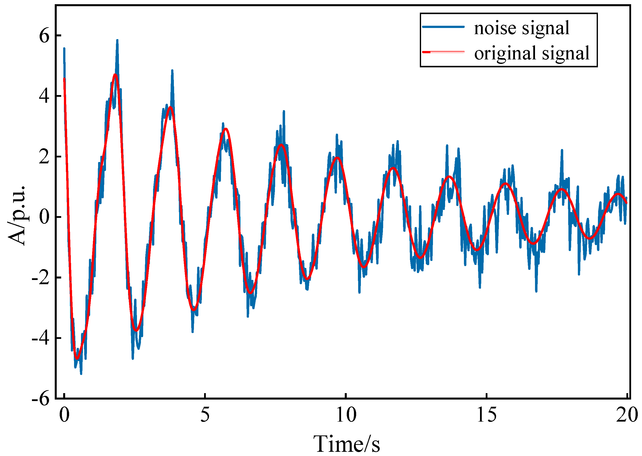
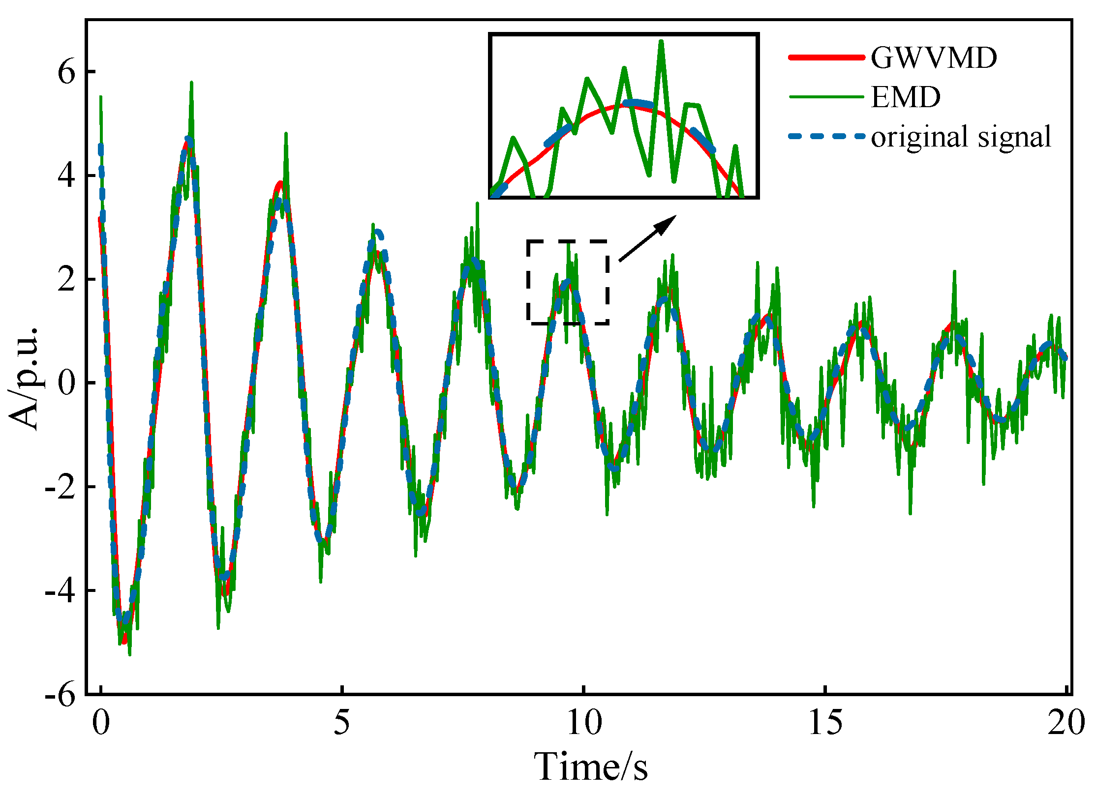
5.1. Numerical Signal Experiment

To confirm the value of the approach presented in this paper, we construct a low-frequency oscillation signal. The damping ratio is 0.0318, 0.0477, and 0.0530, respectively.

$$u(t)=5{\mathrm{e}}^{-0.1t}\cos \left(2\pi \times 0.5t+{60}^{°}\right)+1.5{\mathrm{e}}^{-0.3t}\cos \left(2\pi \times t+{30}^{°}\right)+{\mathrm{e}}^{-0.5t}\cos \left(2\pi \times 1.5t+{45}^{°}\right)+v(t)$$

(25)

where $v(t)$ is a Gaussian white noise with a signal-to-noise ratio of 9.5 dB. The sampling frequency is 25 Hz, and the number of sampling points is 500.

Because the frequency difference between the three modes is small, and the noise interference is mixed in it, it will cause the phenomenon of modal confusion. This is to check the suggested method’s accuracy in the case of low-frequency oscillation with a modal overlap. Figure 3 displays the original numerical simulation signal, where A is the amplitude and dimensionless.

The parameter settings of the gray wolf optimization algorithm (GWO) are given in

Table 1. Main parameter setting of GWO method.

Parameter	Numerical Simulation	Hengshan Power Plant Signal
Number of wolves	60	80
Number of iterations	100	150
Dimensionality	2	2
Upper boundary of k	5000	6000
Lower boundary of k	200	200
Upper boundary of α	10	12
Lower boundary of α	2	2

. The number of decomposition layers is determined to be 5, and the penalty factor is 2500 according to the results of the gray wolf optimization. Figure 4 shows a series of the IMF components of the low-frequency oscillation signal after decomposition by the GWVMD and EMD.

From Figure 4, it can be seen that four eigenmode functions and one residual are generated by the GWVMD decomposition. The first IMF component and the second IMF component after the EMD decomposition show the frequency fluctuation and confusion due to the noise interference. However, the decomposition results of the proposed GWVMD method do not show this phenomenon. This indicates that the GWVMD method can effectively suppress the noise interference and mode confusion and reduce the generation of spurious components.

Figure 5 shows the reconstructed signal after the decomposition of the EMD and GWVMD and the filtering of the remaining residuals, and its indexes are shown in

Table 2. Comparison of each indicator of reconstructed signal.

Method	Component Number	SNR	Coef	MSE
EMD	7	10.1724	0.9312	1.3145
GWVMD	5	21.3372	0.9971	0.7932

. The proposed GWVMD method can greatly suppress the modal confusion and has strong noise immunity.

The accuracy of the method to identify the low-frequency oscillation modal parameters is verified by a simulation. The comparative identification experiments of the modal parameters are carried out using the Prony method, the random decrement method (ITD), the HHT method, and the sparse time-domain method (STD) proposed in this paper, respectively. Because Prony and the other comparison algorithms are more sensitive to the noise of the signal, in order to ensure the objectivity of the simulation results, each method will use the signal after the GWVMD preprocessing as the simulation input signal. The identification results of each method for the low-frequency oscillation signals are shown in

Table 3. Identification results of each method for low frequency oscillation signals.

Method	Type	Frequency	Damping Ratio	Frequency Error	Damping Ratio Error
Prony	Modal 1	0.5034	0.0351	0.0034	0.0033
	Modal 2	1.0177	0.0550	0.0177	0.0073
	Modal 3	1.5401	0.0579	0.0401	0.0049
ITD	Modal 1	0.4973	0.0609	0.0027	0.0027
	Modal 2	0.9927	0.0283	0.0073	0.0194
	Modal 3	1.4807	0.0489	0.0193	0.0041
HHT	Modal 1	0.5031	0.0425	0.0031	0.0107
	Modal 2	1.0086	0.0615	0.0086	0.0138
	Modal 3	1.5162	0.0591	0.0162	0.0061
STD	Modal 1	0.5009	0.0541	0.0009	0.0011
	Modal 2	1.0034	0.0490	0.0034	0.0013
	Modal 3	1.5087	0.0539	0.0087	0.0009

.

From the comparison of the parameters in Table 3, it can be seen that in the case of noise interference and frequency mixing, the methods in this paper are able to extract the characteristic parameters of each mode accurately, and the frequency error and damping error are small. In contrast, the Prony method, random decrement method (ITD), HHT, and other methods have larger errors and lower recognition accuracy. Therefore, the method proposed in this paper can not only accurately extract the low-frequency oscillation characteristic parameters but also has a small overall error of identification. The accuracy of the method for low-frequency oscillation signal identification is proved.

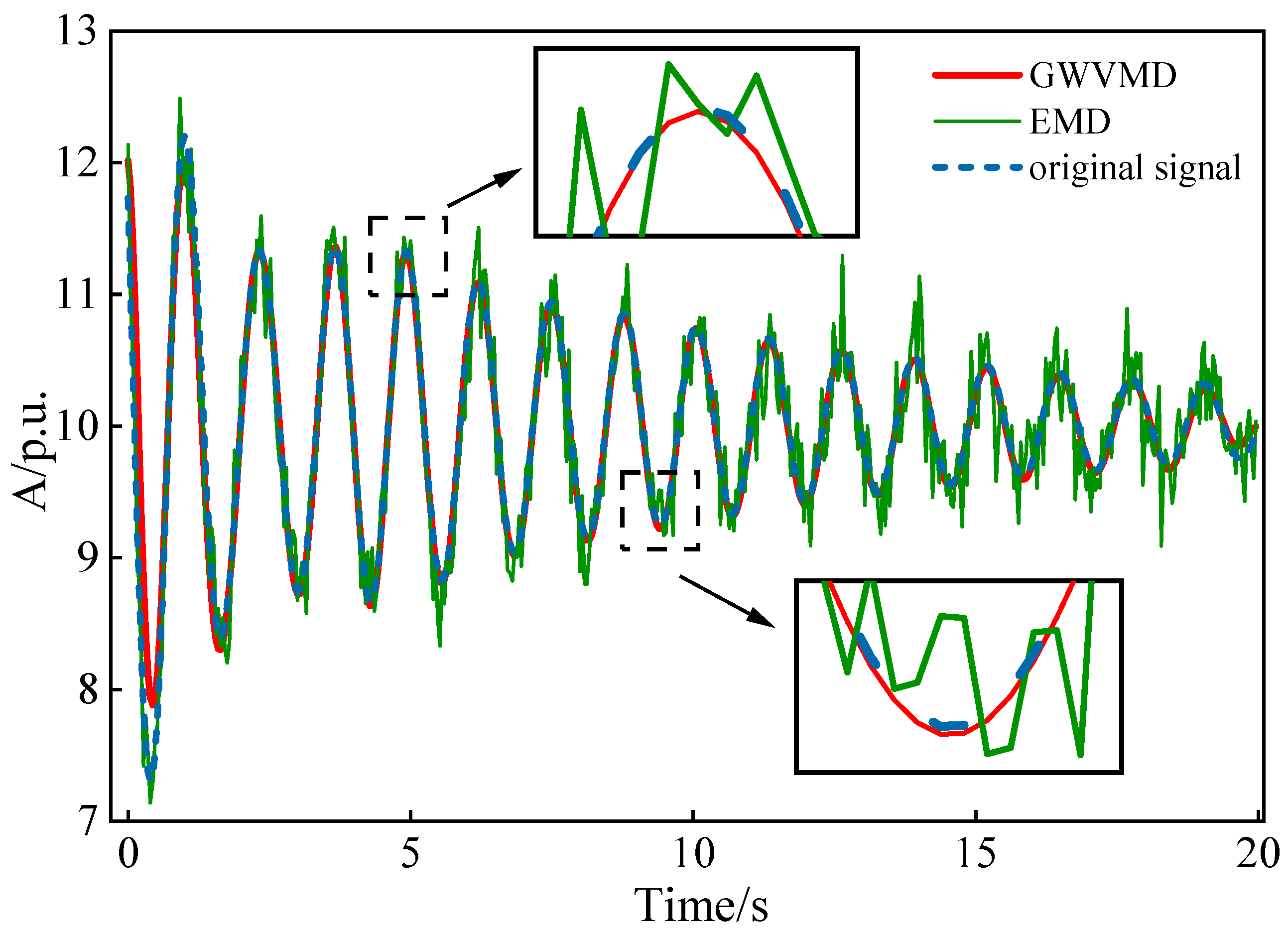
5.2. Hengshan Power Plant Unit Experiment

This paper uses the low-frequency oscillation data of the #1 unit system of the Hengshan power plant for the simulation experiments. The oscillation signal of the relative power angle of unit #1 is collected, and Gaussian white noise with a signal-to-noise ratio of 9.5 dB is added to this low-frequency oscillation signal as the experimental data set. The number of decomposition layers is determined to be four according to the results of the gray wolf optimization, and the calculation determines the quadratic penalty factor to be 3300. The image of the original low-frequency oscillation signal is shown in Figure 6, where A is the amplitude value and dimensionless.

The series of the IMF components obtained by decomposing the noise-containing signal by the EMD and GWVMD, respectively, are shown in Figure 7.

As can be seen from Figure 7, the 1st IMF component decomposed by the EMD is seriously confused in frequency due to the noise interference, which affects the accuracy of the later mode identification. However, under the same noise interference, the GWVMD does not suffer from noise interference, and at the same time, the number of IMF components decomposed by it is less. It is proved that the proposed method can effectively reduce the noise interference, suppress the modal confusion, and reduce the spurious components. Figure 8 shows the reconstructed signal after the decomposition of the oscillation signal. The decomposition performance of each method is shown in

Table 4. Comparison of each indicator of reconstructed signal.

Method	Component Number	SNR	Coef	MSE
EMD	6	16.6903	0.8923	1.9223
GWVMD	4	21.9122	0.9773	1.0817

.

As shown in Table 4, the signal-to-noise ratio of the reconstructed signal processed by the GWVMD can be improved from 9.5 to 21.9122 dB. At the same time, it outperforms the EMD method in many evaluation indexes, such as the correlation coefficient and mean square deviation of the original signal.

In order to verify the noise reduction performance of the GWVMD method, we use the EMVMD [33], PSOVMD [34], and SVDVMD [35] low-frequency oscillation noise reduction methods for the comparison experiments. The experimental results are shown in

Table 5. Noise reduction performance comparison results.

Method	Component Number	SNR	Coef	MSE
EMVMD	5	18.9127	0.9012	1.9223
PSOVMD	5	19.1947	0.9153	1.7037
SVDVMD	4	20.0011	0.9371	1.6939
GWVMD	4	21.9122	0.9773	1.0817

. From Table 5, it can be seen that the signal-to-noise ratio of the reconstructed signals processed by the GWVMD method is improved by 14, 12, and 9%, respectively, compared with the noise reduction methods of the EMVMD, PSOVMD, and SVDVMD. Meanwhile, the correlation between the reconstructed signal and the original signal is higher, and the error is lower. The effectiveness of the gray wolf optimization algorithm for the VMD improvement and noise reduction performance is demonstrated experimentally.

To further confirm the efficiency of the suggested approach, the Prony method, the random subtraction method (ITD), the HHT method, and the sparse time-domain method (STD) of this paper are also chosen to perform the modal discrimination of the noisy voltage amplitude signal, and the results are shown in

Table 6. Identification results of each method for low frequency oscillation signals.

Method	Type	Frequency	Damping Ratio	Frequency Error	Damping Ratio Error
Prony	Modal 1	0.7898	0.0313	0.0113	0.0191
	Modal 2	0.9946	0.0647	0.0134	0.0203
ITD	Modal 1	0.7906	0.0290	0.0121	0.0168
	Modal 2	0.9942	0.0636	0.0130	0.0192
HHT	Modal 1	0.7878	0.0339	0.0093	0.0217
	Modal 2	0.9954	0.0673	0.0142	0.0229
STD	Modal 1	0.7846	0.0246	0.0061	0.0124
	Modal 2	0.9893	0.0591	0.0081	0.0147

.

From the comparison of the results in Table 6, it can be seen that the frequency error and damping error of the method in this paper for the identification of each modal characteristic parameter is smaller compared with the other compared methods when the noise interference is included. The accuracy of the Prony method, the stochastic subtraction method (ITD), and the HHT method for the identification of low-frequency oscillations is lower. Once again, the effectiveness of the proposed method in the identification of low-frequency oscillation modes in actual coal-fired units is demonstrated.

Meanwhile, we choose the latest EFEMD-HT [36], RDT-ERA [37], and TLS-ESPRIT [38] low-frequency oscillation identification methods to conduct the comparison experiments on the noise-laden voltage amplitude signals.

Table 7. Low-frequency oscillation identification comparison results.

Method	Type	Frequency	Damping Ratio	Frequency Error	Damping Ratio Error
EFEMD-HT	Modal 1	0.7868	0.0300	0.0083	0.0178
	Modal 2	0.9919	0.0636	0.0107	0.0192
RDT-ERA	Modal 1	0.7876	0.0305	0.0091	0.0183
	Modal 2	0.9925	0.0641	0.0113	0.0197
TLS-ESPRIT	Modal 1	0.7859	0.0280	0.0074	0.0158
	Modal 2	0.9911	0.0605	0.0099	0.0161
GWVMD-STD	Modal 1	0.7846	0.0246	0.0061	0.0124
	Modal 2	0.9893	0.0591	0.0081	0.0147

shows the low-frequency oscillation identification results of the first two modes in each method. From Table 7, it can be seen that the GWVMD-STD method has an overall reduction of 34, 44, and 21% in the frequency error and 37, 41, and 18% in the damping error compared to the EFEMD-HT, RDT-ERA, and TLS-ESPRIT methods. This is because the GWVMD method effectively reduces the noise interference of the original signal. Meanwhile, the sparse time-domain method (STD) can achieve the multi-channel parameter identification for the noise-reduced signal. The proposed model is experimentally demonstrated to have a high discrimination accuracy for low-frequency oscillation signals.

5.3. Discussions

(1) In order to solve the problems of low accuracy and poor anti-interference of the current low-frequency oscillation mode identification methods for power systems, this paper proposes a low-frequency oscillation mode feature identification method that improves the combination of the variational modal decomposition and sparse time-domain method. We use the gray wolf optimization algorithm (GWO) to determine the important parameters in the variational modal decomposition (VMD), so as to decompose and reconstruct the low-frequency oscillation signal and filter out the noise in the signal. Then, we use the sparse time-domain (STD) method to identify the modal parameters, which improves the identification performance of the STD method.

(2) The gray wolf optimization (GWO) algorithm can find the optimal number of decomposition layers and penalty factor values for the variable modal decomposition. The simulation results of the actual low-frequency oscillation at the Hengshan power plant show that the signal-to-noise ratio of the reconstructed signal processed by the GWVMD method is improved by 14, 12, and 9% compared with the noise reduction methods of the EMVMD, PSOVMD, and SVDVMD, respectively. The correlation between the reconstructed signal and the original signal is higher, and the error is lower. Also, the GWVMD verifies the superiority of the method in the numerical simulation experiments.

(3) The sparse time-domain method can accurately identify the modal parameters in the noise-reduced low-frequency oscillation signal. The actual low-frequency oscillation simulation results of the Hengshan power plant show that the STD method is more accurate than the Prony, ITD, and HHT methods in identifying low-frequency oscillation signals when noise interference is included. The frequency error and damping error of the method for the identification of the characteristic parameters in each mode are smaller. Meanwhile, the numerical simulation experiments also prove that the proposed method has a higher recognition accuracy for low-frequency oscillation signals.

(4) Compared with the EFEMD-HT, RDT-ERA, and TLS-ESPRIT methods in the recent literature, the proposed method reduces the frequency error by 34, 44, and 21% and the damping error by 37, 41, and 18% for the actual low-frequency oscillation signal with a noisy voltage amplitude in the Hengshan power plant. The effectiveness of the proposed method in the identification of low-frequency oscillation modes in practical power systems is further demonstrated.

6. Conclusions

In this paper, a low-frequency oscillation mode feature identification method based on the combination of the adaptive variational modal decomposition (GWVMD) and sparse time-domain method (STD) is proposed. First, an adaptive variational modal decomposition method (GWVMD) is proposed to preprocess the low-frequency oscillation signal of the unit, and the gray wolf optimization (GWO) algorithm is introduced to optimize the variational modal decomposition and find the optimal quantity of the decomposition layers and penalty factor values of the model. Secondly, the noise-reduced processed signal is used as the new input signal, and the sparse time-domain method is used to identify the oscillation modes and their parameters. Finally, the effectiveness of the proposed method is verified by comparing the actual low-frequency oscillation signals of the Hengshan power plant units. The experimental results show that the proposed method is better than various methods such as Prony, ITD, and HHT in the identification of low-frequency oscillation modes and can accurately extract the characteristic parameters of each mode. Meanwhile, the overall frequency error of the method is reduced by 34, 44, and 21%, and the overall damping error is reduced by 37, 41, and 18% compared with the EFEMD-HT, RDT-ERA, and TLS-ESPRIT methods in the recent literature. The excellent performance of the proposed methods in suppressing the modal confusion and noise immunity is demonstrated.

References

1. Ma, J.; Jie, H.; Zhou, Y.; Shao, H.; Zhao, S.; Du, Y.; Wang, J.; Sun, S.; Huang, Y.; Shen, Y. A low frequency oscillation suppression method for grid-connected DFIG with virtual inertia. Int. J. Electr. Power Energy Syst. 2023, 144, 108531. [Google Scholar] [CrossRef]
2. Zou, X.; Du, X.; Tai, H. Stability analysis fo and direct-drive permanent magnet synchronous generator based wind farm integration system considering wind speed. IET Renew. Power Gener. 2020, 14, 1894–1903. [Google Scholar] [CrossRef]
3. Shao, B.; Miao, Z.; Wang, L.; Meng, X.; Chen, Z. Low frequency oscillation analysis of two-stage photovoltaic grid-connected system. Energy Rep. 2022, 8, 241–248. [Google Scholar] [CrossRef]
4. Chen, A.; Ba, Y.; Luo, X.; Huang, H.; Meng, L.; Shi, J. Strategy for grid low frequency oscillation suppression via VSC-HVDC linked wind farms. Energy Rep. 2022, 8, 1287–1295. [Google Scholar] [CrossRef]
5. Chen, G.; Liu, C.; Fan, C.; Han, X.; Shi, H.; Wang, G.; Ai, D. Research on damping control index of ultra-low frequency oscillation in hydro-dominant power systems. Sustainability 2020, 12, 7316. [Google Scholar] [CrossRef]
6. Rudnik, V.; Ufa, R.; Malkova, Y. Analysis of low frequency oscillation in power system with renewable energy sources. Energy Rep. 2022, 8, 394–405. [Google Scholar] [CrossRef]
7. Yu, X.; Zhou, L.; Guo, K.; Liu, Q. A review of research on low frequency oscillation damping control of power systems containing new energy generation access. Chin. J. Electr. Eng. 2017, 37, 6278–6290. [Google Scholar]
8. Pourbeik, P.; Gibbard, M. Damping and synchronizing torques induced on generators by FACTS stabilizers in multimachine power systems. IEEE Trans. Power Syst. 1996, 11, 1920–1925. [Google Scholar] [CrossRef]
9. Kundur, P.; Rogers, G.J.; Wong, D.Y.; Wang, L.; Lauby, M.G. A comprehensive computer program package for small signal stability analysis of power systems. IEEE Trans. Power Syst. 1990, 5, 1076–1083. [Google Scholar] [CrossRef]
10. Li, S.; Ye, C.; Zhang, H.; Chen, D.; Zhu, Z. Overview of power system low frequency oscillation suppression based on DFIG power oscillation damper. Power Constr. 2022, 43, 25–33. [Google Scholar]
11. Chai, H. Research on the Control Strategy of Suppressing Electromechanical Oscillation of Power Grid by Photovoltaic. Master’s Thesis, Shanxi University, Taiyuan, China, 2021. [Google Scholar]
12. Chen, Q.; Fan, D.; Wang, C.; Liu, W.; Yuan, X.; Yuan, X. Small signal model of AC/DC distribution network and analysis of DC side low frequency oscillation. Power Eng. Technol. 2022, 41, 117–125. [Google Scholar]
13. Dang, J.; Liu, D.; Zeng, C. Analysis of power system low frequency oscillation based on normal form theory of vector field. Power Sci. Eng. 2012, 28, 26–31. [Google Scholar]
14. Mu, X.; Jiang, P.; Xu, M.; Cui, J.; Guan, W.; Liu, Z. Parameter identification of excitation system of a 600 MW unit in Heilongjiang based on time domain analysis. Heilongjiang Electr. Power 2019, 41, 495–498. [Google Scholar]
15. Rai, S.; Lalani, D.; Nayak, S.K.; Jacob, T.; Tripathy, P. Estimation of low frequency modes in power system using robust modified Prony. IET Gener. Transm. Distrib. 2016, 10, 1401–1409. [Google Scholar] [CrossRef]
16. Netto, M.; Mili, L. A Robust Prony Method for Power System Electromechanical Modes Identification. In Proceedings of the 2017 IEEE Power & Energy Society General Meeting, Chicago, IL, USA, 16–20 July 2018; IEEE: Piscataway, NJ, USA, 2018. [Google Scholar]
17. Zhu, W.; Ma, J.; Zeng, Z.; Zhou, Y. Low frequency oscillation pattern recognition method based on segmented Fourier neural network. Power Syst. Prot. Control. 2012, 40, 40–45. [Google Scholar]
18. Ge, W.; Yin, X.; Ge, Y.; Qu, C.; Huang, X.; Wang, C. Study on Pattern Recognition Method of Power System Low Frequency Oscillation Based on MEMD and HHT. Power Syst. Prot. Control 2020, 48, 124–135. [Google Scholar]
19. Su, A.; Sun, Z.; He, X.; Zhang, Y.; Wang, C. Power System Low Frequency Oscillation Mode Identification Based on Multivariate Empirical Mode Decomposition. Power Syst. Prot. Control 2019, 47, 113–125. [Google Scholar]
20. Wang, Y. Power System Low Frequency Oscillation Pattern Recognition Based on Deep Learning Algorithm. Master’s Thesis, South China University of Technology, Guangzhou, China, 2017. [Google Scholar]
21. Wang, X. Research on Low Frequency Oscillation Mode Identification of Power System Based on Intelligent Computing. Master’s Thesis, South China University of Technology, Guangzhou, China, 2017. [Google Scholar]
22. Ma, N.; Xie, X.; He, J.; Wang, H. Overview of research on broadband oscillation of power system with high proportion of new energy and power electronic equipment. Chin. J. Electr. Eng. 2020, 40, 4720–4732. [Google Scholar]
23. He, P.; Chen, J.; Geng, S.; Shen, R.; Qi, P. Analysis of Low Frequency Oscillation Characteristics of Interconnected Systems with Wind Power by FACTS Devices. Power Syst. Prot. Control 2020, 48, 86–95. [Google Scholar]
24. Wang, M.; Wu, Y. Simulation research on modal analysis of vibration system based on random decrement method. Electromechanical Technol. 2017, 5, 56–64. [Google Scholar]
25. Li, Z.; Xiang, J.; Sheng, T.; Xiao, B. Time domain weighted sparse constraint space-time adaptive processing algorithm. J. Air Force Univ. Eng. (Nat. Sci. Ed.) 2020, 21, 87–92. [Google Scholar]
26. Han, R.; Teng, Y.; Xie, J.; Wang, X.; Che, Y. Low frequency oscillation identification of power system based on improved STD method. Power Autom. Equip. 2019, 39, 58–63. [Google Scholar]
27. Shen, Z.; Ding, R. A Novel Neural Network Approach for Power System Low Frequency Oscillation Mode Identification. In Proceedings of the 2019 IEEE International Symposium on Circuits and Systems (ISCAS), Sapporo, Japan, 26–29 May 2019; IEEE: Piscataway, NJ, USA, 2019. [Google Scholar]
28. Yan, H.; Hwang, J.; Gao, Y. Power system low frequency oscillation modal parameter identification based on noise like data. Power Gener. Technol. 2022, 43, 19–31. [Google Scholar]
29. Si, W.; Li, S.; Xiao, H.; Li, Q. PD characteristics and development degree assessment of oil-pressboard insulation with ball-plate model under 1:1 combined AC-DC voltage. IEEE Trans. Dielectr. Electr. Insul. 2017, 24, 3677–3686. [Google Scholar] [CrossRef]
30. Song, Y.; Liu, G.; Zhu, L.; Wang, J. Application of Improved Grey Wolf Optimization Algorithm in SVM Parameter Optimization. Sens. Microsyst. 2022, 41, 151–155. [Google Scholar]
31. Wu, T.; Sun, K.; Shi, W. Research on cable partial discharge noise reduction based on AVMD adaptive wavelet packet method. Power Syst. Prot. Control. 2020, 48, 95–103. [Google Scholar]
32. Wu, H.; Zhu, C.; Zhang, Y.; Long, Y. An adaptive typical day selection method based on improved fuzzy clustering algorithm. Smart Power 2022, 50, 60–67. [Google Scholar]
33. Yong, T. Study on Power System Oscillation of Hydroelectric Units Containing High Permeability. Master’s Thesis, Northeastern Electric Power University, Jilin, China, 2020. [Google Scholar]
34. Cheng, Y.; Ping, H.; Zhu, Y. Research on low-frequency oscillation of power system based on optimized VMD-HT algorithm. J. Jiangxi Electr. Power Vocat. Tech. Coll. 2022, 35, 7–10. [Google Scholar]
35. Ouyang, Z. Research on the Analysis Method of Power System Pan-Band Oscillation Based on the Measured Signal. Master’s Thesis, Hunan University, Changsha, China, 2020. [Google Scholar]
36. Zhang, C.; Qiu, B.; Liu, J. Low-frequency oscillation mode identification of power system based on EFEMD-HT energy method. South. Power Grid Technol. 2022, 16, 48–57. [Google Scholar]
37. Zeng, X.; Xiao, H.; Wang, H.; Liu, J. Low-frequency oscillation mode parameter identification based on RDT and ERA algorithm. J. Electr. Power 2018, 33, 471–477. [Google Scholar]
38. Zhu, J. Low-frequency oscillation mode identification of power system based on improved TLS-ESPRIT. Electr. Switch 2021, 59, 64–67. [Google Scholar]
Figure 1. GWVMD method process steps.
Sustainability 14 16867 g001
Figure 2. Overall flow chart of low-frequency oscillation mode identification.
Sustainability 14 16867 g002
Figure 3. Image of the original signal after adding noise.
Sustainability 14 16867 g003
Figure 4. Components of the decomposed low-frequency oscillation signal. (a) Signal after EMD decomposition. (b) Signal after GWVMD decomposition.
Sustainability 14 16867 g004
Figure 5. Reconstructed signal after decomposition by different methods.
Sustainability 14 16867 g005
Figure 6. Relative power angle oscillation signal.
Sustainability 14 16867 g006
Figure 7. Components of the decomposed low-frequency oscillation signal. (a) Signal after EMD decomposition. (b) Signal after GWVMD decomposition.
Sustainability 14 16867 g007
Figure 8. Reconstructed signal of low-frequency oscillation.
Sustainability 14 16867 g008