Multi-Aircraft Cooperative Strategic Trajectory-Planning Method Considering Wind Forecast Uncertainty

Abstract

We address the issue of multi-aircraft cooperative strategic trajectory planning in free-route airspace (FRA) in this study, taking into consideration the impact of time-varying and altitude-varying wind forecast uncertainty. A bi-level planning model was established in response to the properties of the wind. The upper level focused on minimizing the flight time, while the lower level aimed to reduce potential conflicts. Meanwhile, a heuristic approach based on conflict severity (CS) within the framework of a cooperative co-evolution evolutionary algorithm (CCEA) was proposed to accelerate the convergence speed in view of the complexity of this optimization issue. In order to conduct the experiments, historical data of 1479 flights over western Chinese airspace were retrieved. The number of conflicts, total flight time, total flight time variance, and deviation were used as indicators to evaluate the safety, efficiency, and predictability of the trajectory. When compared to a trajectory in the structured airspace, the optimal solution was conflict-free and reduced the total flight time by about 17.7%, the variance by 11.7%, and the deviation by 37.5%. Additionally, the contrast with the two-stage model demonstrated that the proposed method was entirely meaningful. The outcome of this survey can provide an effective trajectory-planning method, which is crucial for the sustainable development of future air traffic management (ATM).

1. Introduction

Increasing air traffic is expected in the coming decades, impacting flight efficiency and safety. The IATA estimates that the worldwide passenger number will reach 7.3 billion, according to its 20-year forecast to 2034. The IATA forecasts that, by 2034, 1.8 billion additional passengers will travel to, from, and within the Asia-Pacific region, with an overall market size of 2.9 billion. The size will carry 42% of all world traffic, with an average annual growth rate of 4.9% [1]. An unavoidable barrier to achieving the sustainable development of the air transportation system is the imbalance between the expanding air traffic demand and the constrained capacity of the airspace.

Against this backdrop, the need to modernize the air transportation system is evident. Prominent initiatives have been launched both in Europe (i.e., SESAR) and in the US (i.e., NextGen) to develop a future air transportation system that is more flexible, resilient, and scalable than that of today [2]. The implementation of both the ICAO free-route airspace [3] and trajectory-based operation [4] concepts serves as the cornerstone of these endeavors. In FRA, users freely plan a route between a defined origin and destination, with the possibility of routing via intermediate points, which is more flexible. With the shift toward TBO, aircraft need to meet strict time and space constraints in the form of four-dimensional trajectory (4DT) [5]. In this framework, more accurate trajectory information can be provided for ATM.

Trajectory planning is a crucial subject in ATM from the operational point of view. According to the studied time horizon, trajectory planning can be classified into strategic (usually considering at network scale), pre-tactical, and tactical (usually considering only a sector). Under the paradigm of TBO, it is realizable to conduct trajectory planning in the strategic stage. Due to the coupling relationship between aircraft, tactical trajectory planning may create a “domino” effect, keeping the trajectory planning in a reactive state and endangering airspace safety. For example, when we modify departure time to resolve potential conflicts, a delayed aircraft may still need to wait for many other aircraft to meet the capacity constraints [6]. Strategic trajectory planning, however, may not only provide the optimal solution from a global perspective and lessen the workload of air traffic controllers, but it may also resolve the problem of large-scale trajectory planning.

Because of the extensively studied time horizon and broad flight span, there is no doubt that uncertainty factors cannot be discarded in strategic trajectory planning. There are several different sources of uncertainty that impact ATM, from participant choices to ambiguity and unavailability of the trajectory data [7]. Wind direction and speed, fog, snowfall, and thunderstorms are some of the weather-related factors that have significant effects on ATM systems. 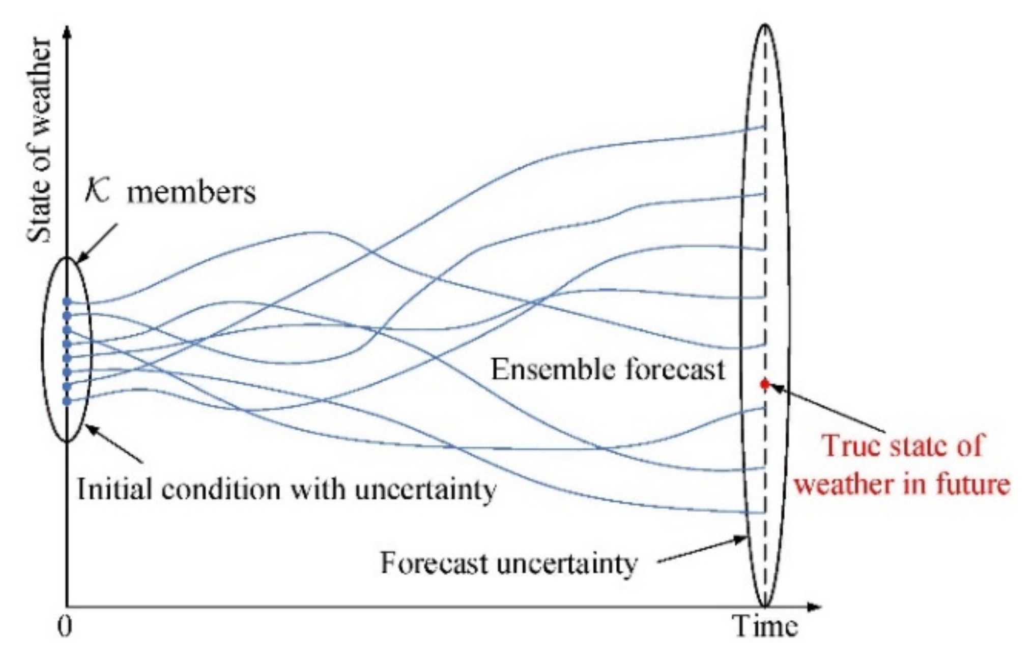Incomplete knowledge of current and future weather conditions is responsible for aircraft delays and cancellations, which negatively affects ATM systems and converts into additional costs for airlines and air navigation service providers [8]. The trend today for describing and quantifying inherent forecast uncertainty is ensemble prediction systems (EPSs), which are based on ensemble modeling [9].

Numerous studies have used EPSs to account for weather forecast uncertainty in order to enhance the robustness of trajectory planning. Gonzalez-Arribas et al. suggested combining a robust optimal control framework with probabilistic forecasts generated by an EPS [10,11]. A straightforward strategy is to take into account each EPS member independently, apart from this. Legrand [12] applied the Bellman algorithm to each member to obtain the optimal trajectory ensemble, based on which a hierarchical clustering algorithm was proposed to obtain a robust optimal trajectory from the ensemble. Although complex in terms of computation, this approach was accurate. Therefore, it was not appropriate for cooperative trajectory planning issues. On the other hand, extending some of the probabilistic trajectory prediction approaches is a frequent strategy. The optimal solution is, therefore, discovered using a discrete optimization method [13,14]. A Dijkstra-based trajectory predictor based on a deterministic trajectory prediction system was transformed into a probabilistic trajectory prediction system by Cheung et al. [15]. For the purpose of optimizing trajectory over the north Atlantic, Franco et al. [9] integrated the Dijkstra algorithm with a probabilistic trajectory predictor based on a suggested probabilistic transformation approach. Additionally, using a mixed-integer linear-programming method, they created a multi-objective mathematical model in a structured airspace while taking wind uncertainty information into account in [16]. The author noted that this method was equally adapted to FRA. This approach was more effective in solving a large-scale trajectory planning problem compared to the former.

In trajectory planning, ensuring the safety of the aircraft is as essential as improving efficiency. Several efforts have been made in the past to address the problem of conflict detection and resolution (CD&R) under the presence of weather forecast uncertainty. An approach is to propagate the uncertainty from the source into the trajectory prediction. Rodionova et al. [17] studied five types of CD&R models considering uncertainty based on EPSs. Hernández-Romero [8,18] supposed that the wind components followed a four-parameter β distribution. The probabilistic conflict detection problem was tackled using a probabilistic transformation method and the probability distribution of the aircraft position was derived based on the joint distribution of the wind components. The limitation was that the wind was constant within a certain area in their research. The trajectory uncertainty can be accurately captured by the probabilistic transformation approach, but the computational complexity is insufficient for large-scale problems and strategic CD&R. Another common method assumes that the aircraft location or flight time follows a predefined probability distribution and treats it as a random variable. According to Jacquemart [19], the motion of an aircraft consisted of a deterministic motion and a three-dimensional Brownian motion perturbation, with the variance increasing with time. To enhance the accuracy of conflict probability estimates while predicting the probability of collision, the authors implemented an interacting particle system. Guan [20] used a Gaussian distribution to represent the location of an aircraft. In this article, the authors made the supposition that aircraft were independent of one another and that the probability density function (PDF) solely related to the moment when the aircraft arrived at the segment’s origin. A multiple CD&R model was suggested by Jilkov et al. [21] that took intention and weather uncertainty into account, modeling the separation vector between two aircraft as a Gaussian mixed distribution. By linearly distributing the arrival time deviation of an aircraft to its waypoints, Courchelle [22] investigated the impact of weather uncertainty on CD&R. The expected arrival time and the deviation were used to calculate the arrival time interval at each waypoint. However, the potential conflicts were solved only by adjusting the aircraft speed. Dai [23] also utilized an uncertainty radius to represent the unknowable uncertainty of the aircraft. However, it was challenging to estimate the magnitude and was not accurate enough to manage uncertainty.

The presented studies have usually assumed the wind uncertainty as constant. However, strategic trajectory planning has an extensive time span. Inevitably, wind changes over time as a flight progresses. The time-varying nature of wind can cause the planned optimal trajectory to be non-optimal and adversely affect CD&R efficiency. Furthermore, existing studies have often performed the route planning and CD&R separately. Nevertheless, in CD&R, the corresponding conflict resolution strategy may lead to a change in the optimal route. For example, the optimal route fluctuates owing to time-varying wind when a departure time adjustment strategy is adopted.

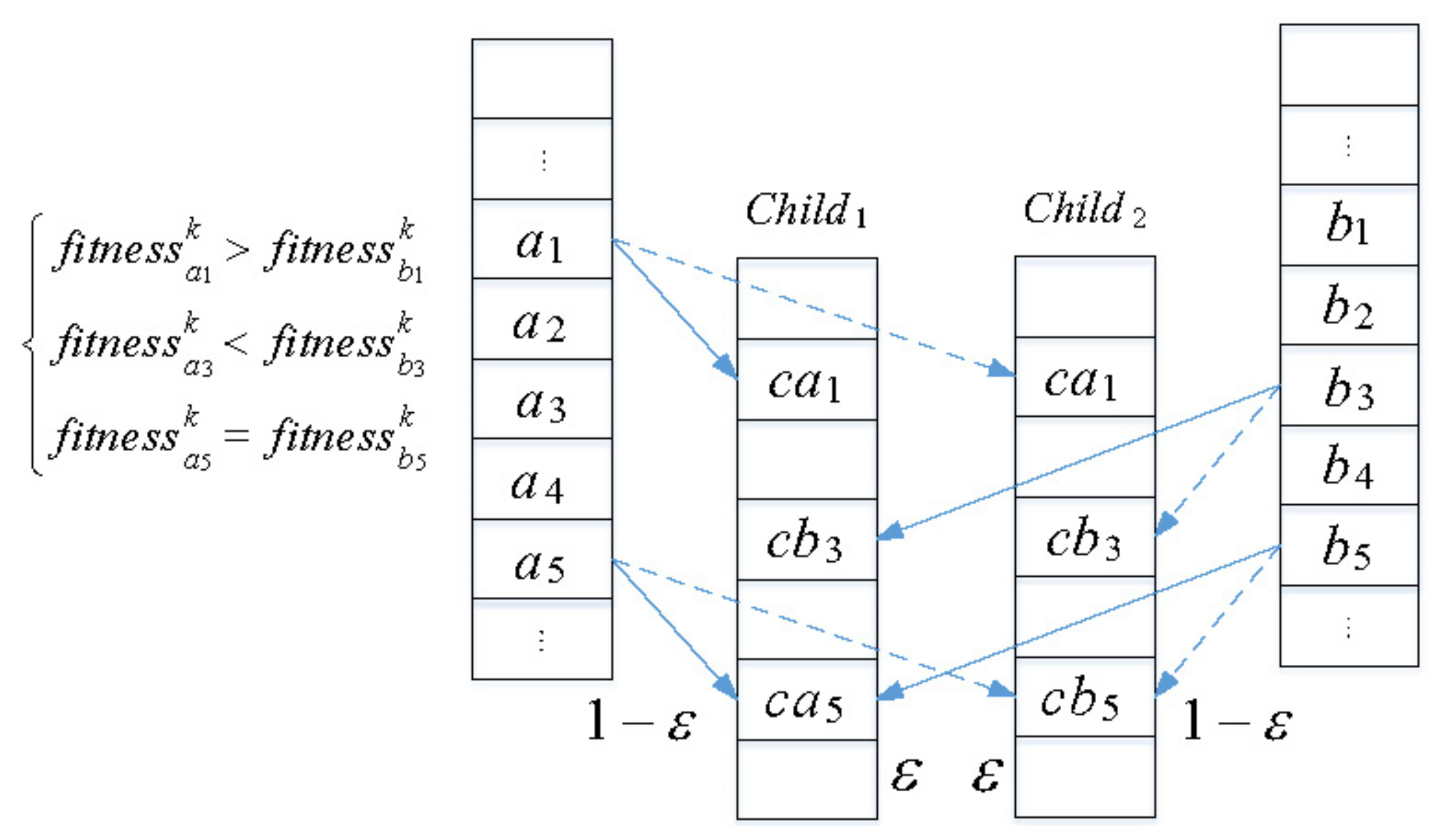
To address the problems above, this paper proposes a bi-level programming model based on EPSs taking time-varying and altitude-varying wind forecast uncertainty into account. In order to integrate aircraft efficiency and safety, the upper level optimizes the route, and the lower level performs CD&R. To solve the problem quickly, a heuristic strategy based on conflict severity is designed under the framework of a cooperative co-evolution evolutionary algorithm [24]. Simulation validation is performed using flights over the western Chinese airspace from 8:00 a.m. to 12:00 p.m. on 8 June 2019, and the experiment results show the proposed model and algorithm have good benefits.

The structure of this essay is as follows: The ensemble trajectory prediction model is introduced in Section 2. In Section 3, we describe the bi-level mathematical model and how it was applied to the issue of trajectory planning. The methods employed in the upper and lower model are described in Section 4; Section 5 presents the results analysis. Finally, in Section 6, we conclude with a brief discussion of the work.

2. Ensemble Trajectory Prediction

A probabilistic weather prediction model is the most suitable one for strategic trajectory planning in order to account for inherent weather unpredictability. The use of probability forecasting enables users to make decisions based on quantified weather uncertainty, which contributes to the socio-economic benefits [16]. Applying EPSs to represent forecast uncertainty is now popular. Accordingly, one of the important strategies for examining trajectory uncertainty is ensemble trajectory prediction [15].

2.1. Time-Varying and Altitude-Varying Wind and Forecast Uncertainty

An EPS generates a forecast ensemble by running a numerical weather prediction system $\mathcal{K}$ times, each time with a different starting state and physical parameter. For example, PEARP (France) contains 35 members; MOGREPS (UK) has 12 members; the ECMWF (Europe) consists of 51 members; and the multi-model ensemble SUPER, formed by the combination of the previous three, is constructed of 98 members. Each member represents a possible future weather condition [15], as shown in Figure 1.

Figure 1. Ensemble prediction system.

The integrated forecasting system of the ECMWF is an ensemble of 51 members (1 control member and 50 perturbed members). The ECMWF has a forecast up to 15 days, with two times per day at 0000UTC and 1200UTC. The horizontal interval is 32 km, and the vertical direction is divided into 91 layers [25].

A wind grid was constructed to store the wind information provided by the EPS. The size was $N\times M$, with a step ${\Delta }_{lat}$ in latitude and ${\Delta }_{lon}$ in longitude. The grid ranged from ${\lambda }_{\min }$ to ${\lambda }_{\max }$ in latitude and from ${\varphi }_{\min }$ to ${\varphi }_{\max }$ in longitude, as shown in Figure 2. Each grid node stored information, including latitude $\lambda$, longitude $\varphi$, altitude $h$, the east wind component $W_E$, and the north wind component $W_N$.

Figure 2. Wind grid.

When the studied time span was [0, T], the forecasting wind data was given at the time interval $t_{\mathrm{vp}}$, starting from the moment of 0. The wind was variable in time and vertical dimension, and the moment when the wind changes was called the time-varying point. Undoubtedly, $W_E(t)$ and $W_N(t)$ were related to time. In Figure 3, on 8 June 2019, the trends of $W_E(t)$ and $W_N(t)$ from 8:00–12:00 at $\left(31°\mathrm{N},93°\mathrm{E}\right)$ with an altitude of 10,100 m and the trends of $W_E(t)$ and $W_N(t)$ from 8900–11,600 m at 8:00 are given.

Figure 3. The trends of $W_E(t)$ and $W_N(t)$ from 8:00–12:00 at $\left(31°\mathrm{N},93°\mathrm{E}\right)$ (altitude 10,100 m) and the trends from 8900 m–11,600 m at 8:00 (red dot represents the wind speed).

At each grid point, the wind bearing ${\theta }_w(t)$ is shown in Figure 4a, ${\theta }_w(t)$ and the wind norm $‖\overrightarrow{W}(t)‖$ was calculated with the following formula:

$$\begin{array}{l}{ \theta }_w(t)=\arctan \left\{\frac{W_E(t)}{W_N(t)}\right\}\\ ‖\overrightarrow{W}(t)‖=\sqrt{W_E^2(t)+W_N^2(t)}\end{array}$$

(1)

Figure 4. Wind bearing (a) and segment bearing (b), red (waypoint), green (wind).

In strategic trajectory planning, due to the long advance time and the large span of the aircraft operation time, it is necessary to consider the critical effect of time-varying and the altitude-varying wind.

2.2. Time-Varying Ensemble Trajectory Prediction Model

According to Dancila [26], choosing a geographic area is a crucial decision in trajectory planning since it influences both the effectiveness of the algorithm and the optimal solution. For the multi-aircraft collaborative trajectory-planning problem, the entry and exit points into and out of FRA cover a wide area. Hence, a rectangular geographical area [27] was constructed.

In this work, the latitude and longitude ranges of the geographical search area were consistent with the wind grid and had the same grid granularity. The grid nodes formed the waypoint set $\mathcal{W}$. Each node had a list of allowed neighbors, which are represented by the black links in Figure 5. These links formed the segment set $ℰ$. The available altitude set was defined as $\mathscr{H}$. Therefore, $\forall h\in \mathscr{H}$, and the FRA could be modeled as a graph $\mathcal{G}(\mathcal{W},\mathcal{E})$.

Figure 5. Waypoint connection rule: current waypoint (red), allowed (blue), and disallowed (green).

Let us consider a set of flights $\mathcal{F}$ scheduled to pass over a given FRA in [0, T]. Then, $\forall f\in ℱ,h\in \mathscr{H}$, and the 4DT could be described as $\left\{\right(e_f^1,h_f,{\mathcal{T}}_f^{e^1}),\{(e_f^2,h_f,{\mathcal{T}}_f^{e^2}),\dots ,(e_f^n,h_f,{\mathcal{T}}_f^{e^{\mathrm{n}}})\}$: where $e_f^i$ is the segment $i$ aircraft $f$ passed; $h_f$ is the corresponding flight altitude; and ${\mathcal{T}}_f^{e^i}$ is the flight time set on segment $e_f^i$. When $r_f$ is the horizontal route of the aircraft $f$, then it can be expressed as a sequence of $n$ segments, i.e.:

$$\begin{array}{l} r_f=\left(e_f^1,\dots ,e_f^n\right),\\ e_f^i\in ℰ, e_f^{i-1}\in {\stackrel{=}{ℰ}}_{e_f^i},e_f^{i+1}\in \underset{=}{ℰ}{e}_f^i,\\ e_f^i=(w_f^i,w_f^{i+1}),w_f^i\in \mathcal{W}\end{array}$$

where ${\stackrel{=}{ℰ}}_{e_f^i}$ is the set of segments entering the tail node of segment $e_f^i$, and $\underset{=}{ℰ}{e}_f^i$ is the set of outgoing segments from the head node. ${ℰ}_{e_f^i}={\stackrel{=}{ℰ}}_{e_f^i}\cup \underset{=}{ℰ}{e}_f^i$ is the set of segments connected to the blue nodes in Figure 5.

$T_f^{e^i}$ was obtained by ensemble trajectory prediction. We considered a three-degree-of-freedom point-mass model of a commercial aircraft flying over the FRA, with the assumption that the aircraft was in the cruise part with a constant speed and altitude.

$\forall e\in ℰ$ connected one origin node $w_o$ and the destination node $w_d$. The great circle distance of segment $e$ was given by the following formula:

$$d^e=R\cdot \arccos \left({\overrightarrow{P}}_d\cdot {\overrightarrow{P}}_o\right)$$

(2)

where

$$\begin{array}{l}{\overrightarrow{P}}_o={\left(X_o,Y_o,Z_o\right)}^T\\ {\overrightarrow{P}}_d={\left(X_d,Y_d,Z_d\right)}^T\end{array}$$

(3)

${\overrightarrow{P}}_o$ and ${\overrightarrow{P}}_d$ are the Cartesian coordinates of the nodes $w_o$ and $w_d$, respectively. Assuming $R$ is the radius of the Earth indicates the vector inner product. For a given waypoint $w$, the Cartesian coordinates were given by the following formula:

$$\overrightarrow{P}=\left\{\begin{array}{l}X=R\cdot \cos (\lambda )\times \cos (\varphi )\hfill \\ Y=R\cdot \cos (\lambda )\times \sin (\varphi )\hfill \\ Z=R\cdot \sin (\varphi )\hfill \end{array}\right.$$

(4)

The segment bearing ${\theta }_e$ is shown in Figure 4b and was calculated by the following formula:

$$\left\{\begin{array}{l}{\theta }_e\left(w_o,w_d\right)=\arctan \left(\frac{y}{x}\right)\hfill \\ y=\sin \left({\varphi }_d-{\varphi }_o\right)\cdot \cos \left({\lambda }_d\right)\hfill \\ \begin{array}{l}x=\cos \left({\lambda }_o\right)\cdot \sin \left({\lambda }_d\right)-\\ \sin \left({\lambda }_o\right)\cdot \cos \left({\lambda }_d\right)\cdot \cos \left({\varphi }_d-{\varphi }_o\right)\end{array}\hfill \end{array}\right.$$

(5)

Based on the previous equation, we now computed the tail wind for the origin $w_o$ and destination $w_d$ of segments $e$ (${VW}_o^e(t)$ and ${VW}_d^e(t)$):

$$\begin{array}{l}{VW}_o^e(t)=‖\overrightarrow{W_o}(t)‖\cdot \cos \left({\theta }_e-{\theta }_{w_o}(t)\right)\\ {VW}_d^e(t)=‖\overrightarrow{W_d}(t)‖\cdot \cos \left({\theta }_e-{\theta }_{w_d}(t)\right)\end{array}$$

(6)

The two tail winds were then averaged and associated with each segment:

$${VW}^e(t)=\frac{{VW}_o^e(t)+{VW}_d^e(t)}{2}$$

(7)

Then, for each segment, the time needed by the aircraft to connect node $w_o$ and $w_d$ was:

$$T^e(t)=\frac{d^e}{V_a+{VW}^e(t)}$$

(8)

where $V_a$ is the true airspeed of the aircraft.

The deterministic trajectory prediction method was repeatedly applied to each member of the EPS. Consequently, we could obtain some parameter sets of the trajectory, such as flight time, fuel consumption, and so on.

According to the above-mentioned segment flight time calculation method, under the condition of member $k$, we could calculate the flight time ${(T_k^e(t))}_f$. Finally, the flight time set ${\mathcal{T}}_f^e(t)=((T_1^e(t){)}_f,(T_2^e(t){)}_f,T_3^e(t){)}_f,\cdots ,T_{\mathcal{K}}^e(t){)}_f)$ could be obtained, and $\mathcal{K}$ was the number of EPS members. Based on the assumption that each member in the EPS had the same probability of occurring, the flight cost of the segment could be defined as the mean [28], the deviation, or a linear combination of any other characteristics [29].

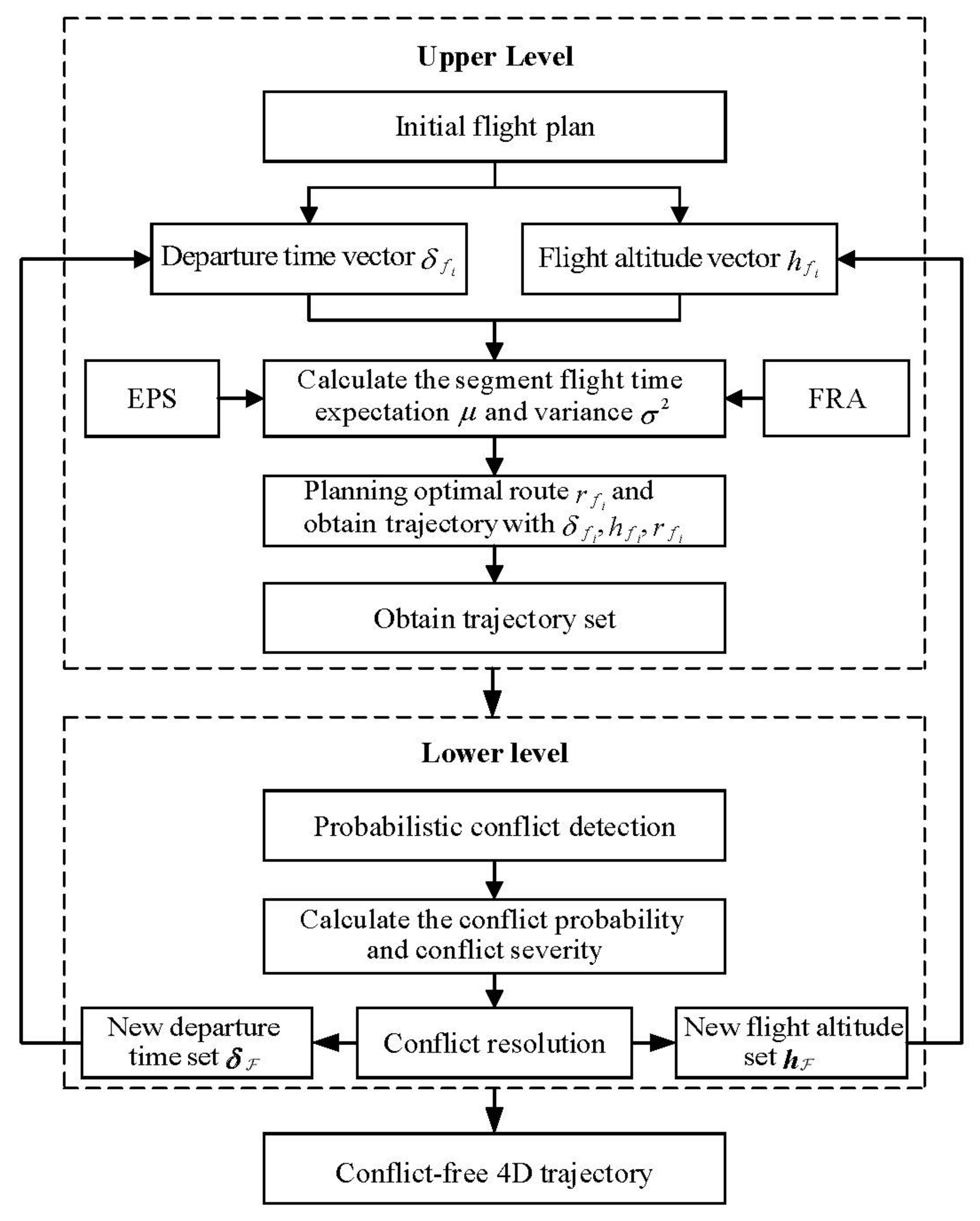
3. Trajectory-Planning Model

Based on the analysis of time-varying and altitude-varying wind and forecast uncertainty, a bi-level trajectory planning model was established. This model integrated the efficiency and safety of aircraft, with the aircraft departure time and flight altitude as the trigger conditions. The upper level focused on the aircraft optimal route planning, and the objective of the lower-level programming was to minimize the conflict number and trajectory amendment cost for conflict resolution. A flow chart of the model is shown in Figure 6.

Figure 6. Bi-level programming model flow chart.

3.1. Assumptions

In this work, the following assumptions were considered:

• The time $\Delta T$ from the departure moment to the entry moment of the flight entering the FRA was constant and known;
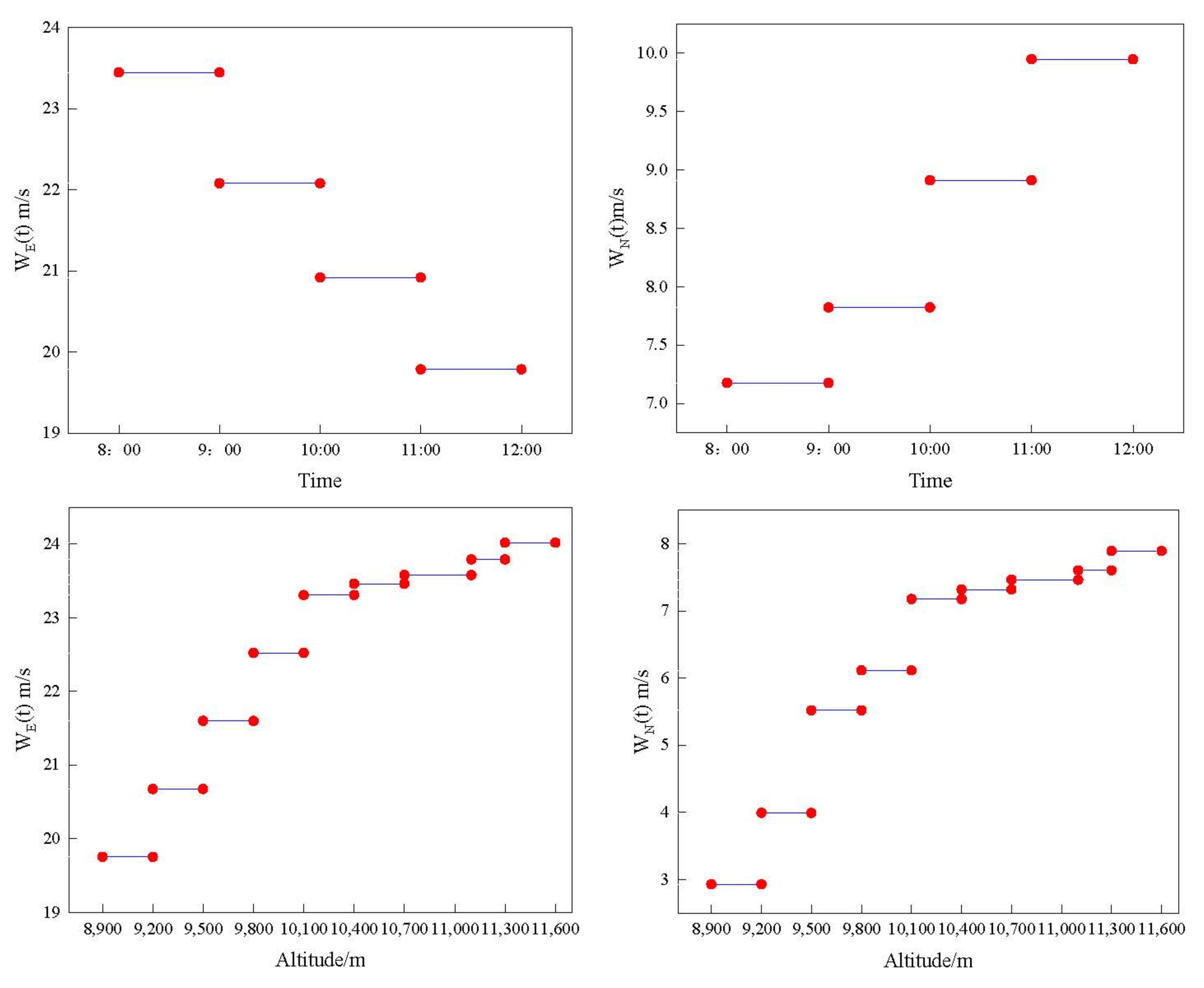
• The segment flight time was related to the moment when the aircraft arrived at the beginning of the segment only, ignoring the effect of wind change over a segment;
• The segment flight time variance and maximum error in arrival time at the end of the segment grew linearly with flight time;
• The PDFs of the flight times on different segments were independent, and the PDFs between different aircraft were independent, too.

3.2. The Upper Level for Route Planning

The effect of time-varying and altitude-varying wind was considered in the route planning. The objective of the upper-level programming was to minimize the expected flight time of the route with a variance constraint. Therefore, the optimal route must satisfy two requirements: the shortest flight time and the allowed predictability.

$\forall f\in ℱ,h\in \mathscr{H}$, $e\in r_f$ under the influences of wind, the unbiased estimates of the flight time expectation ${\mu }_{f,h}^e(t)$, and variance ${{\sigma }^2}_{f,h}^e(t)$ could be obtained from ${\mathcal{T}}_{f,h}^e(t)$ from Section 2.2:

$${\widehat{\mu }}_{f,h}^e(t)=\frac{1}{\left|\mathcal{K}\right|}{\displaystyle \mathbf{\sum }_{k=1}^{\left|\mathcal{K}\right|}}(T_k^e(t){)}_{f,h},{\widehat{\sigma }}_{ f,h}^{2e}(t)=\frac{1}{\left|\mathcal{K}\right|-1}{\displaystyle \mathbf{\sum }_{k=1}^{\left|\mathcal{K}\right|}}((T_k^e(t){)}_{f,h}-{\widehat{\mu }}_{f,h}^e(t){)}^2$$

(9)

We defined the time arriving at the start of the segment as $t_{f,h}^{oe}$ and the time departing the end of the segment as $t_{f,h}^{de}$, resulting in the following:

$$\begin{array}{l}{t}_{f,h}^{oe}={\delta }_f+\Delta T+{\displaystyle \mathbf{\sum }_{\tilde{e}\in \widetilde{ℰ}}}{\widehat{\mu }}_{f,h}^{\tilde{e}}(t), \\ t_{f,h}^{de}=t_{f,h}^{oe}+{\widehat{\mu }}_{f,h}^e(t)\end{array}$$

(10)

where ${\delta }_f$ is the departure time, $\Delta T$ is known, and $\widetilde{ℰ}$ represents the set of segments passed through by $f$ before segment $e$.

As shown in Figure 7, there were two continuous segments of $e^i$ and $e^{i+1}$ in the FRA, and $f$ may be affected by Wind1 and Wind2, where the assumed effective times of Wind1 and Wind2 are $[0,t_{\mathrm{vp}}]$ and $[t_{\mathrm{vp}},{2t}_{\mathrm{vp}}]$, respectively.

Figure 7. No time-varying point on the segment (a) and the presence of time-varying point on the segment (b).

Firstly, on segment $e^i$, as shown in Figure 7a, the aircraft was under the influence of Wind1. If $t_{f,h}^{o{e}^i}<t_{vp}$ and $t_{f,h}^{{de}^i}<t_{vp}$, then we defined no time-varying point. On the contrary, as shown in Figure 7b, if $t_{f,h}^{o{e}^i}<t_{vp}$ and $t_{f,h}^{{de}^i}\ge t_{vp}$, then there was a time-varying point.

In the first situation, the wind did not change on segment $e^i$ and $e^{i+1}$, and aircraft $f$ was influenced by Wind1, yielding the following:

$$\begin{array}{l}{\overline{T}}_{f,h}^{e^i}(t)={\mu }_{f,h,1}^{e^i}(t),{{\sigma }^2}_{f,h}^{e^i}(t)={{\sigma }^2}_{f,h,1}^{e^i}(t)\\ {\overline{T}}_{f,h}^{e^{i+1}}(t)={\mu }_{f,h,1}^{e^{i+1}}(t),{{\sigma }^2}_{f,h}^{e^{i+1}}(t)={{\sigma }^2}_{f,h,1}^{e^{i+1}}(t)\end{array}$$

In the second situation, aircraft $f$ was influenced by Wind1 on segment $e^i$ and influenced by Wind2 on segment $e^{i+1}$, resulting in the following:

$$\begin{array}{l} {\overline{T}}_{f,h}^{e^i}(t)={\mu }_{f,h,1}^{e^i}(t),{{\sigma }^2}_{f,h}^{e^i}(t)={{\sigma }^2}_{f,h,1}^{e^i}(t),\\ {\overline{T}}_{f,h}^{e^{i+1}}(t)={\mu }_{f,h,2}^{e^{i+1}}(t),{{\sigma }^2}_{f,h}^{e^{i+1}}(t)={{\sigma }^2}_{f,h,2}^{e^{i+1}}(t)\end{array}$$

Obviously, Wind1 and Wind2 were in connection with the flight altitude $h_f$, and $t$ was associated with ${\delta }_f$.

According to the previous inference discretizing the overall time range [0, T] into the time set, we could calculate the functions for ${\overline{T}}_{f,h}^e(t)$ and ${{\sigma }^2}_{f,h}^e(t)$.

The departure time and flight altitude were obtained from the lower level, i.e., ${\delta }_f^{up}={\delta }_f^{low}$, $h_f^{up}=h_f^{low}$. Then, the upper-level programming model could be described as $\forall f\in ℱ$, planning the flight time optimal route with variance constraint ${\sigma }_0^2$ when the departure time ${\delta }_f$ and the flight altitude $h_f$ were known.

To formulate the problem, the following decision variable was defined:

$$x_{f,h}^e(t)=\left\{\begin{array}{l}1,\mathrm{if} f \mathrm{is} \mathrm{on} \mathrm{segment} e \mathrm{at} \mathrm{altitude} h \mathrm{by} time t\\ 0,\mathrm{else}\end{array}\right.$$

Then, the vector $X_{f,h}(t),=[x_{f,h}^{e^1}(t),x_{f,h}^{e^2}(t),\dots ,x_{f,h}^{e^{\left|\mathcal{E}\right|}}(t)],t\in \mathcal{T}$ represented the segment status by time $t$. Moreover, the dimension of the vector was equal to the segment number.

The upper-level programming model was as follows:

$$\begin{array}{cc}\hfill & min{\displaystyle \sum _{e\in \mathcal{E},t\in \mathcal{T}}}{\overline{T}}_{f,h}^e\left(t\right)x_{f,h}^e\left(t\right)\hfill \end{array}$$

$$\begin{array}{cc}\hfill & s.t. t(x_{f,h}^e\left(t\right)-x_{f,h}^e(t-1))={\delta }_f \forall f\in \mathcal{F},h\in \mathcal{H},t\in \mathcal{T}:e={orig}_f\hfill \end{array}$$

(11)

$$\begin{array}{cc}\hfill & x_{f,h}^e\left(t\right)\le {\displaystyle \sum _{e^{\prime }\in \stackrel{=}{\mathcal{E}}{e}_f}}{x}_{f,h}^{e^{\prime }}(t+{\overline{T}}_{f,h}^e\left(t\right)) \forall f\in \mathcal{F},h\in \mathcal{H},t\in \mathcal{T}:e\ne {dest}_f\hfill \end{array}$$

(12)

$$\begin{array}{cc}\hfill & x_{f,h}^e(t+{\overline{T}}_{f,h}^{e^{\prime }}\left(t\right))\le {\displaystyle \sum _{e^{\prime }\in \underset{=}{\mathcal{E}}{e}_f}}{x}_{f,h}^{e^{\prime }}\left(t\right) \forall f\in \mathcal{F},h\in \mathcal{H},t\in \mathcal{T}:e\ne {orig}_f\hfill \end{array}$$

(13)

$$\begin{array}{cc}\hfill & {\displaystyle \sum _{e\in \mathcal{E},t\in \mathcal{T}}}{\sigma }_{f,h}^{2^e}\left(t\right)x_{f,h}^e\left(t\right)\le {\sigma }_0^2 \forall f\in \mathcal{F},h\in \mathcal{H}\hfill \end{array}$$

(14)

$$\begin{array}{cc}\hfill & {\displaystyle \sum _{t\in \mathcal{T}}}{x}_{f,h}^e\left(t\right)\le 1 \forall f\in \mathcal{F},h\in \mathcal{H},e\in \mathcal{E}\hfill \end{array}$$

(15)

$$\begin{array}{cc}\hfill & {\displaystyle \sum _{e\in \mathcal{E}}}{x}_{f,h}^e\left(t\right)=1 \forall f\in \mathcal{F},h\in \mathcal{H},t\in \mathcal{T}\hfill \end{array}$$

(16)

where constraint (11) imposes that the aircraft needs to satisfy the allowed departure time. Constraints (12) and (13) indicate that the entry and exit points cannot be changed. In addition, constraint (14) states that the variance does not exceed the acceptable range, constraint (15) is used to ensure that the optimal route does not contain cycles; and constraint (16) indicates that, at any moment, the aircraft must select a segment (that is, $‖X_{f,h}(t)‖=1$).

$$\mathrm{In} \mathrm{general}, \forall t\in \mathcal{T}, e_{f,h}\left(t\right)=X_{f,h}·\mathcal{E}, r_{f,h}=\{e_{f,h}(t_1),e_{f,h}(t_2),\cdots ,e_{f,h}(t_n)\}.$$

3.3. The Lower Level for Probabilistic Strategic CD&R

In the lower-level programming model, the number of conflicts was minimized by ground delay and altitude changes.

Under the context of 4DT, a set of 4D points ${\mathcal{S}}_f$ was obtained by sampling the trajectory at equal distance intervals, i.e.:

$$S_f=\left\{\left({lon}_f^1,{lat}_f^1,h_f^1,T_f^1\right),\right.\left({lon}_f^s,{lat}_f^s,h_f^s,T_f^s\right),\cdots ,\left.\left({lon}_f^{\left|S_f\right|},{lat}_f^{\left|S_f\right|},h_f^{\left|S_f\right|},T_f^{\left|S_f\right|}\right)\right\}$$

(17)

where $\left|{\mathcal{S}}_f\right|$ denotes the number of sample points. ${lon}_f^s$ and ${lat}_f^s$ represent the longitude and latitude of the sample point, respectively; $h_f^s$ is the flight altitude; and $T_f^s$ is obtained from the set ${\mathcal{T}}_{f,h}^e(t)$ mentioned in Section 2.2, indicating the PDF of the aircraft crossing time of the sample point $s$.

3.3.1. Conflict Number and Conflict Severity

Due to the wind forecast uncertainty, an approach to statistically quantifying the severity of aircraft conflict was presented, and we employed the conflict probability (CP) as an indicator to identify the conflict. Then, the conflict number (CN) could be calculated as follows:

$$\begin{array}{c} \mathit{CN}={\displaystyle \sum _{i=1}^{\left|\mathcal{F}\right|}}{\displaystyle \sum _{\underset{j>i}{i=1}}^{\left|\mathcal{F}\right|}}C(S_{f_i},S_{f_j})\\ \mathit{if}\left|\right|({\mathit{lon}}_{f_i}^{S_i},{\mathit{lat}}_{f_i}^{S_i}),({\mathit{lon}}_{f_j}^{S_j},{\mathit{lat}}_{f_j}^{S_j})|{|}_2<N_{ h,}\\ |h_{f_i}^{S_i}-h_{f_j}^{S_j}|N_{ v},{\mathit{CP}}_{f_i,f_j}\ge {\mathit{CP}}_0,\\ \mathit{then}: \\ C(S_{f_i},S_{f_j})=1\end{array}$$

(18)

where $N_h$ is the horizontal separation, $N_v$ is the vertical separation, and ${CP}_0$ is the maximum acceptable conflict probability.

According to the upper-level programming model, the expectation of the flight time on segment $e$ was ${\overline{T}}_{f,h}^e$, and the variance was ${{\sigma }^2}_{f,h}^e$, defining the maximum error in the arrival time at the end of the segment as follows:

$$\begin{array}{c}\begin{array}{c}{\omega T}_{f,h}^e=\max \left\{({\omega T}_{f,h}^e{)}_{\min },({\omega T}_{f,h}^e{)}_{\max }\right\}\\ where:\left({\omega T}_{f,h}^e\right)\min ={\overline{T}}_{f,h}^e-\underset{k\in \mathcal{K}}{\min }\left(\right(T_k^e{)}_{f,h})\\ ({\omega T}_{f,h}^e{)}_{\max }=\underset{k\in \mathcal{K}}{\max }(\left(T_k^e{)}_{f,h}\right)-{\overline{T}}_{f,h}^e\end{array}\end{array}$$

(19)

If there was no time-varying point on $e$, then:

$$\begin{array}{c}\begin{array}{c}\forall {\overline{t}}_{f,h}^s\in \left[t_{f,h}^{oe},t_{f,h}^{de}\right],({\omega t}_{f,h}^e{)}^s=\frac{{\overline{t}}_{f,h}^s-t_{f,h}^{oe}}{t_{f,h}^{de}-t_{f,h}^{oe}}\times {\omega T}_{f,h}^e+{\displaystyle \sum _{\tilde{e}\in \tilde{\mathcal{E}}}}{\omega T}_{f,h}^{\tilde{e}},\\ ({\sigma }^{2_{f,h}^e}{)}^s=\frac{{\overline{t}}_{f,h}^s-t_{f,h}^{oe}}{t_{f,h}^{de}-t_{f,h}^{oe}}\times {\sigma }_{f,h}^{2^e}+{\displaystyle \sum _{\tilde{e}\in \tilde{\mathcal{E}}}}{\sigma }^{2_{f,h}^{\tilde{e}}}.\end{array}\end{array}$$

(20)

If there was a time-varying point on $e$ (Figure 7b), then the segment was divided into two sub-segments at the time-varying point. In addition, the time-varying point must be contained in the sample point set ${\mathcal{S}}_f$. The crossing-time expectation and variance in the sample point on the sub-segments could be calculated by Equation (20).

We considered aircraft $f_1$ with sample point $s_1$, as well as aircraft $f_2$ with sample point $s_2$. Under the assumption that the crossing time, in general, obeyed a Gaussian distribution, $T_{f_1}^{s_1}$ and $T_{f_2}^{s_2}$ could be acquired, where the expectation and variance were calculated by Equations (19) and (20).

Then, the joint PDF was:

$$T_{f_1,f_2}^{s_1,s_2}(t)=T_{f_1}^{s_1}(t)\times T_{f_2}^{s_2}(t)$$

(21)

The CP and conflict time (CT) are shown in Figure 8 and were determined with the following equation:

$$\begin{array}{c}\begin{array}{c}CP={\int }_{{DT}_1}^{{DT}_2}{T}_{f_1,f_2}^{s_1,s_2}\left(t\right)dt,CT={\int }_{{DT}_1}^{{DT}_2}t{T}_{f_1,f_2}^{s_1,s_2}\left(t\right)dt\\ {DT}_1=\min ({\overline{t}}_{f_1,h_1}^{s_1}+{\omega t}_{f_1,h_1}^{s_1},{\overline{t}}_{f_2,h_2}^{s_2}-{\omega t}_{f_2,h_2}^{s_2}),{DT}_2=\max ({\overline{t}}_{f_1,h_1}^{s_1}+{\omega t}_{f_1,h_1}^{s_1},{\overline{t}}_{f_2,h_2}^{s_2}-{\omega t}_{f_2,h_2}^{s_2})\end{array}\end{array}$$

(22)

where $[{DT}_1,{DT}_2]$ is the overlap of the time intervals.

Figure 8. Conflict probability and conflict time.

The conflict severity (CS) was the sum of the CTs of two aircrafts’ total sample points, i.e.:

$$CS={\displaystyle \sum _{S_{f_i},S_{f_j}}}CT$$

(23)

3.3.2. Conflict Resolution Model

The decision variable in the lower-level programming was:

$$u: =(\delta ,h)$$

where $\delta : =\left({\delta }_1,{\delta }_2,{\delta }_3,\cdots ,{\delta }_{\left|ℱ\right|}\right)$ is the departure time vector, and $h: =\left(h_1,h_2,h_3,\cdots ,h_{\left|ℱ\right|}\right)$ is the flight altitude vector.

In order to deviate from the optimal trajectory as little as possible, we defined the trajectory amendment cost (TAC), which consisted of the ground delay cost ($C_{GD}$) and the flight altitude changes cost ($C_{FA}$). In this paper, $C_{GD}$ and $C_{FA}$ were normalized. The TAC was calculated as follows:

$$\begin{array}{l}TAC={\chi }_{GD}\times C_{GD}+{\chi }_{FA}\times C_{FA}\\ C_{GD}={\displaystyle \sum _{f\in ℱ,h\in \mathscr{H}}}\left({\delta }_f-{\delta }_f^{orig}\right)\\ C_{FA}={\displaystyle \sum _{f\in ℱ,h\in \mathscr{H}}}\left|h_f-h_f^{orig}\right|\end{array}$$

(24)

where ${\chi }_{GD}$ and ${\chi }_{FA}$ represent the ground delay and flight altitude changes cost weights, respectively.

Then, the objective function in the upper-level programming was:

$$objective=\max \left\{\frac{1-TAC(u)/{TAC}_{\max }}{1+CN(u)}\right\}$$

The following constraints should be satisfied in this model:

• Ground delay constraint: With the aim to prevent the flight from being postponed too long, the ground delay ${GD}_f$ was be limited to lie in the discrete interval $[0,{\Delta T}_{GD}]$:

  $$\begin{array}{c}\forall f\in ℱ,G{D}_f\in \left\{0,\Delta t_{GD},\dots ,\Delta T_{GD}\right\}\\ G{D}_f={\delta }_f-{\delta }_f^{orig} \end{array}$$

  (25)

  where ${\Delta t}_{GD}$ is the ground delay slot; ${\Delta T}_{GD}^{}$ represents the maximum acceptable delay; and ${\delta }_f$ and ${\delta }_f^{orig}$ are the real and initial departure times, respectively.
• Flight altitude constraint: In order to limit the change in flight altitude, the set of all the possible flight altitude changes was set to the following:

  $$\begin{array}{l}\forall f\in ℱ,F{A}_f\in \left\{0,\Delta h_{FA},\dots ,\Delta H_{FA}\right\}\\ F{A}_f=\left|h_f-h_f^{orig}\right|\end{array}$$

  (26)

  where ${\Delta h}_{FA}$ is the flight altitude slot; ${\Delta H}_{FA}^{}$ represents the maximum allowed change; and $h_f$ and $h_f^{orig}$ are the real and initial flight altitudes, respectively.
  In general, the lower-level programming model was:

  $$\begin{array}{l} max \frac{1-TAC(u)/{TAC}_{\max }}{1+CN(u)}\\ s.t. G{D}_f\in \left\{0,\Delta t_{GD},\dots ,\Delta T_{GD}\right\}\\ F{A}_f\in \left\{0,\Delta h_{FA},\dots ,\Delta H_{FA}\right\}\end{array}$$

  (27)

4. Algorithms

Trajectory planning is a large-scale combinatorial optimization problem, which is often solved by heuristic algorithms. The successful implementation of this bi-level methodology largely depended on developing efficient solution algorithms. In this work, a genetic algorithm (GA) and a CCEA were used to optimize the upper- and lower-level programming models, respectively. Moreover, a heuristic strategy based on CS was designed to accelerate the convergence of the CCEA. The framework is described in Algorithm 1.

Algorithm 1: The framework of the proposed method.

Input: Historical data, MAXgenerations

Output: Conflict free 4D trajectory

//Upper level

1: Planning the optimal initial route with GA according to the decision variables;

2: Obtain the optimal trajectory set;

//Lower level

3:For i = 1: MAXgenerations do

4:  Resolve the potential conflicts with CCEA and obtain new decision variable;

5:  Recalculate optimal trajectory set with upper level according to new decision variable.

6:End for

4.1. GA for Upper-Level Optimization

4.1.1. Chromosome Structure

As described in Section 2, the grid nodes were firstly numbered in the orders of east to west and south to north. Then, the route $r_f$ could be represented as a set of node sequences. Therefore, when solving the model with the GA, we used an integer-coding method and sorted the nodes in temporal order. The chromosome structure is shown in Figure 9.

Figure 9. Chromosome structure.

4.1.2. Initialized Population

The population, in terms of possible routes, should respect the following constraints:

• The aircraft could only fly to adjacent waypoints;
• The entry and exit points in the FRA could not be changed.

4.1.3. Route Crossover

In this paper, a one-point crossover method was used. According to the connection rule shown in Figure 5, it could be classified into two cases. When the crossover solution satisfied the connection rule, then a valid route was obtained, as depicted in Figure 10a; on the contrary, an invalid route was created, as shown in Figure 10b. A tournament selection mechanism was employed to randomly choose two parents from the population.

Figure 10. Valid crossover route (full line, (a)) and invalid crossover route (dotted line, (b)), red dot represents the waypoint.

4.1.4. Route Mutation

We used a one-point mutation method, and the mechanism is shown in Figure 11, where the solid line indicates a valid mutation route, and the dashed line indicates an invalid mutation route.

Figure 11. Valid mutation route (full line) and invalid mutation route (dotted line), red dot represents the waypoint.

4.2. CCEA for Lower-Level Optimization

A CCEA was originally proposed by Potter [30]. In applying a CCEA, the complexity of a large-scale optimization problem is reduced by decomposing it into multiple sub-problems according to a certain grouping strategy, including uniform grouping, random grouping, and variable grouping based on domain knowledge [31]. Each sub-problem is evolved by an individual evolutionary algorithm. A complete problem solution is acquired by assembling the representative members from each sub-population. CCEAs and their improvements have been successfully applied in ATM.

As discussed above, the flights were divided according to a dynamic grouping strategy design based on their interdependence. In the process of sub-problem optimization, we used a fast GA [32] with a CS strategy. The framework was as follows (Algorithm 2):

Algorithm 2: CCEA

Input: Initial solution, MAXgenerations, maxgenerations

Output: CCEA solution

//Main procedure

1:Initialize the initial solution based on CS to generate the initial population;

2:for i = 1: MAXgenerations do

3:  Evaluate all the individuals in the population and select the best one based on the

4:  fitness matrix;

//Cooperative co-evolution

5:  Decompose the best solution into mi sub-problems based on the dynamic

6:  grouping strategy;

7: Set j = 1

8: while j ≤ mi do

9:    for k = 1: maxgenerations do

10:      Initialize the jth sub-population;

11:      Select the offspringk based on the fitness matrix;

12:        Use the adaptive crossover and mutation strategy to obtain the offspringk+1;

13:    end for

14:   j = j + 1

15: end while

16:end for

4.2.1. Dynamic Grouping Strategy

First of all, we defined a matrix $\mathcal{C}\mathcal{S}$ to indicate the CSs between two flights:

$$\begin{array}{cc}\hfill & \mathcal{C}\mathcal{S}=\left(\begin{array}{ccc}C{S}_{11}& \cdots & C{S}_{1\left|\mathcal{F}\right|}\\ ⋮& ⋮& ⋮\\ C{S}_{\left|\mathcal{F}\right|1}& \cdots & C{S}_{\left|\mathcal{F}\right|\left|\mathcal{F}\right|}\end{array}\right)\hfill \end{array}$$

(28)

where ${CS}_{ij}$ represents the CS between $f_i$ and $f_j$.

Secondly, a conflict interaction matrix $\mathcal{C}\mathcal{I}$ was defined to denote whether two flights conflicted with each other:

$$\begin{array}{cc}\hfill & \mathcal{C}\mathcal{I}=\left(\begin{array}{ccc}C{I}_{11}& \cdots & C{I}_{1\left|\mathcal{F}\right|}\\ ⋮& ⋮& ⋮\\ C{I}_{\left|\mathcal{F}\right|1}& \cdots & C{I}_{\left|\mathcal{F}\right|\left|\mathcal{F}\right|}\end{array}\right),C{I}_{ij}=\left\{\begin{array}{cc}1,& if C{S}_{ij}>0\\ 0,& if C{S}_{ij}=0\end{array}\right.\hfill \end{array}$$

(29)

If $\forall i\ne j, {CI}_{ij}=0$, a uniform grouping strategy was applied to divide the aircraft into $m$ groups with the same size.

If $\exists i\ne j, {CI}_{ij}=1$, the flights were divided into different groups according to their conflict interactions:

$$\begin{array}{l}{group}^k=\left(f_1^k,f_2^k,\cdots ,f_{\left|{ℱ}_k\right|}^k\right)\\ 0<\left|{ℱ}_k\right|<\left|ℱ\right|,\sum \left|{ℱ}_k\right|=\left|ℱ\right|\end{array}$$

(30)

The flights in each group satisfied the following correlation:

$$\begin{array}{l}\exists f_i,f_j\in {group}^k, {CI}_{ij}=1,\\ \forall f_i\in {group}^k,f_j\in {group}^l, {CI}_{ij}=0.\end{array}$$

(31)

4.2.2. Adaptive Initialization Operator

According to matrix $\mathcal{C}\mathcal{S}$, the CS of $f_i$ was:

$${CS}_i={\displaystyle \sum _{j=1}^{\left|ℱ\right|}}{CS}_{ij}$$

(32)

To select the flight to participate in the initialization, a roulette selection method was used, and preference was given to flights with bigger CSs.

We assume that the probability of adjusting departure time was $P_{GD}$, and the probability of changing flight altitude was $P_{FA}$. Firstly, we randomly generated a number $r,0<r\le 1$. Then, there were two possible cases: if $0<r\le P_{GH}$, we performed the operation of ground delay, and if $P_{GH}<r\le 1$, we changed the flight altitude.

In addition, since each sub-population contained a different number of flights (chromosome size), the number of perturbations was determined according to the size during initialization. The process is shown in Figure 12.

Figure 12. Sub-population initialization.

4.2.3. Adaptive Crossover Operator

The local fitness of each gene in the chromosome, which was determined by the TAC and conflict number of each flight, was offered as an alternative to taking into account a global fitness. The local fitness of each flight was defined as follows:

$${fitness}_j^k=\frac{1-{TAC}_j^k/{TAC}_{max}}{1+{CN}_j^k}$$

(33)

where ${fitness}_j^k$ indicates the fitness of aircraft $j$ in group $k$, and ${TAC}_{max}$ represents the maximum acceptable cost. $a$ and $b$ are selected as parents from the population. If we compared the fitness of the same aircraft from the two parents, the adaptive crossover operator could include the following three cases, as shown in Figure 13:

If ${fitness}_{a_j}^k<{fitness}_{b_j}^k$, the two children inherited from $b_j$, accordingly.

If ${fitness}_{a_j}^k>{fitness}_{b_j}^k$, the two children inherited from $a_j$, accordingly.

If ${fitness}_{a_j}^k={fitness}_{b_j}^k$, the two children were calculated with Equation (34):

$$\begin{array}{l}{ca}_j=floor\left(\epsilon a_j+\left(1-\epsilon \right)b_j\right)\\ {cb}_j=floor\left(\epsilon b_j+\left(1-\epsilon \right)a_j\right)\end{array}$$

(34)

where $floor$ denotes the downward rounding strategy, and $\epsilon$ is the linear recombination coefficient. The crossover probability is $P_c$.

Figure 13. Adaptive crossover operator, child1 (solid lines), child2 (dashed lines).

4.2.4. Adaptive Mutation Operator

It can be concluded from Figure 14 that, if ${fitness}_j^k<\xi$, the mutation operator was performed with probability $P_m$.

Figure 14. Adaptive mutation operator.

5. Case Study

5.1. Database and Experimental Setup

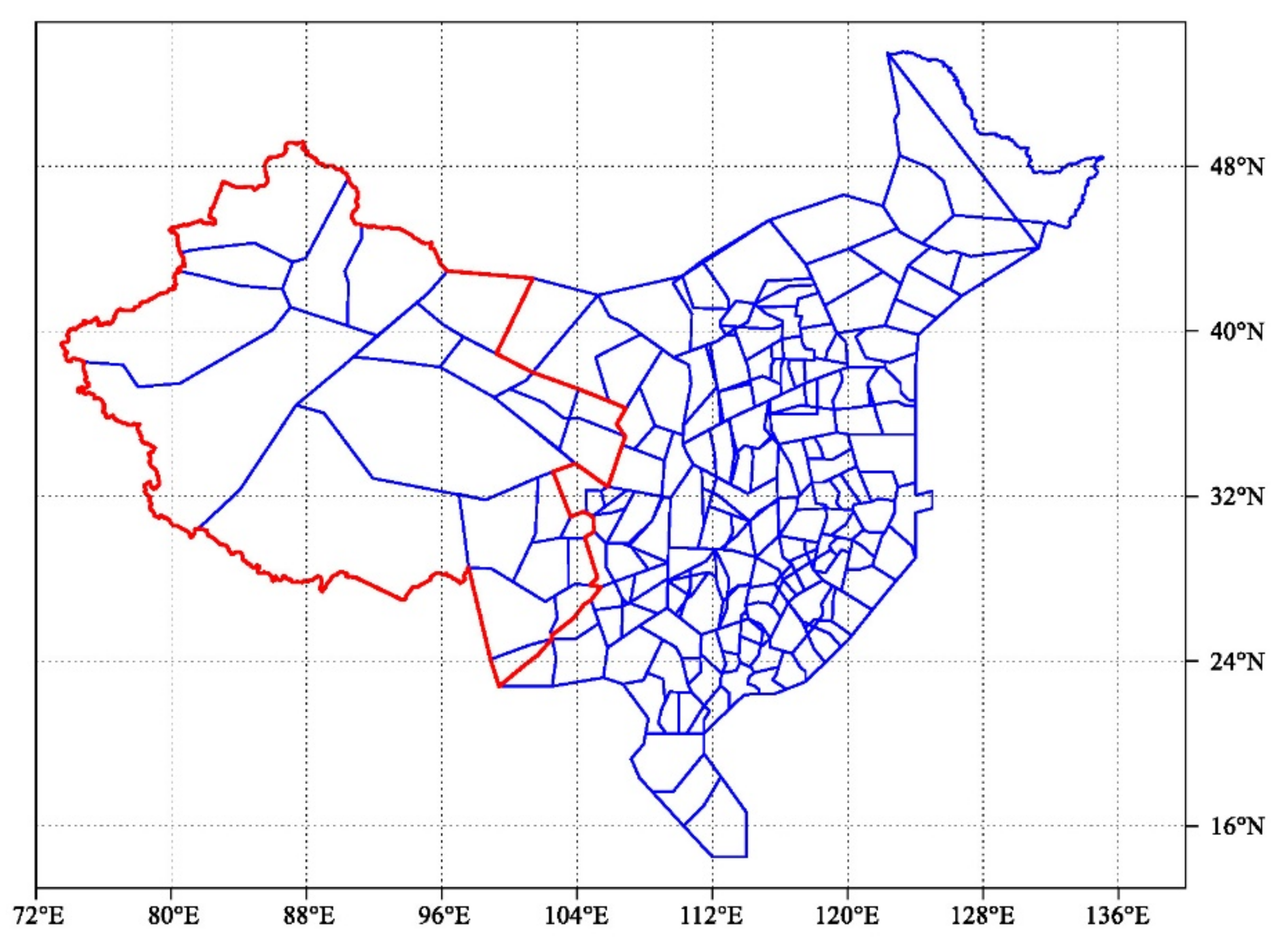
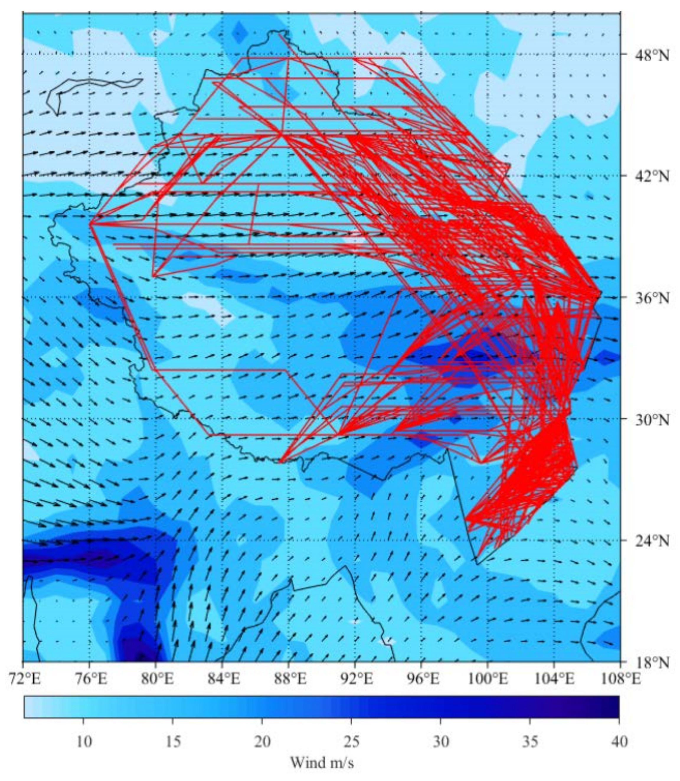
The dataset corresponded to air traffic over western Chinese airspace on 8 June 2019 between 8:00 a.m. and 12:00 p.m. Figure 15 displays the position of the western Chinese airspace. The entry moments into the FRA and altitude distributions of the resulting 1479 flights are shown in Figure 16. Influenced by time-varying wind, the conflicts calculated according to the trajectories in the structured airspace and great circle trajectories are depicted in Figure 17, where the reference wind was the mean value within 4 h (arrow indicates wind value and wind direction, and color represents the deviation of the wind).

Figure 15. The location of western Chinese airspace.

Figure 16. The distribution of the entry times and cruise flight altitudes.

Figure 17. The distribution of routes (red) and conflicts (yellow).

In the process of conflict resolution, the maximum delay of flight ${\Delta T}_{GD}^{}$ was 30 min, and the time slot was 3 min. The altitude range was separated every 300 m, from 8900 m to 11,600 m. The maximum allowed altitude adjustment ${\Delta L}_{FA}^{}$ was 1200 m.

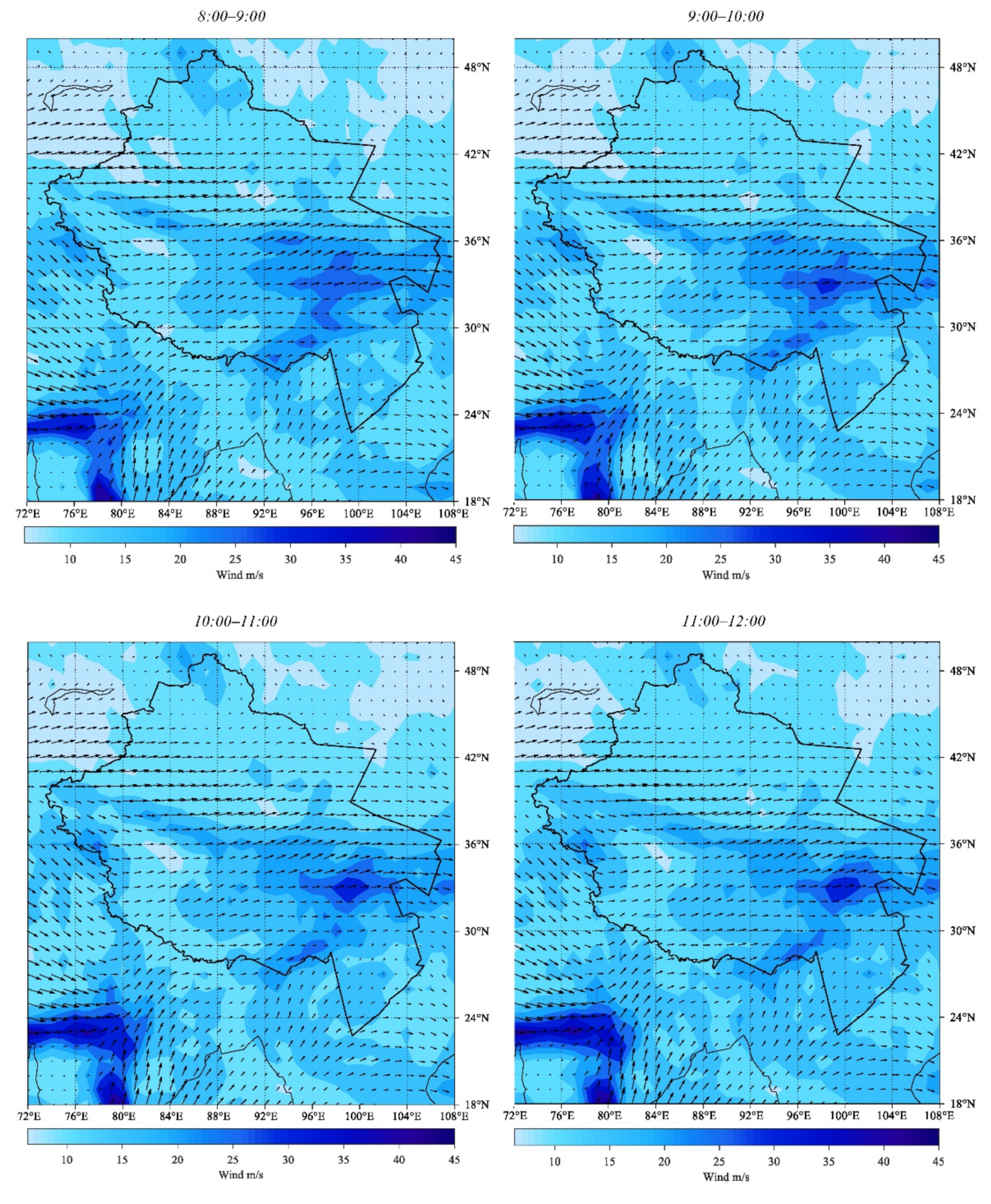
Wind data were obtained from the ECMWF for 8 June 2019 between 8:00 a.m. and 12:00 p.m., with a look-ahead time of 24 h. The wind grid had a granularity of 0.2° and covered the longitude range of 72° E to 108° E, as well as the latitude range of 22° N to 50° N. Figure 18 gives information on the wind at a 10,100 m altitude over 4 h. As we can see, the wind tended to weaken, and the wind uncertainty steadily increased.

Figure 18. The wind in western Chinese airspace between 8:00 a.m. and 12:00 p.m. on 8 June 2019.

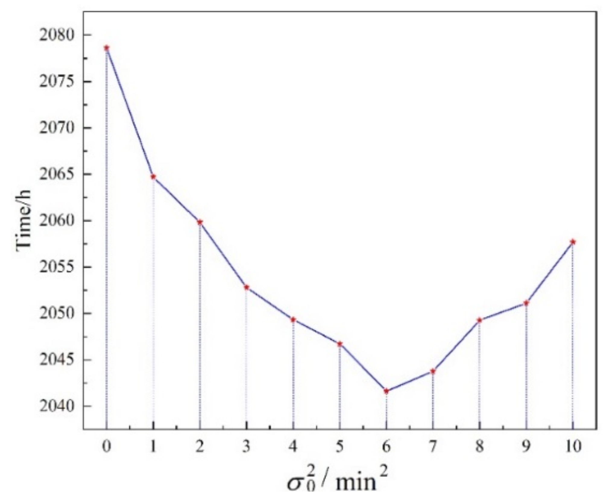
5.2. Parameter Settings and Sensitivity Analysis

The ${\sigma }_0^2$ needed to be sensitivity analyzed for our proposed method. In this section, the sensitivity analysis was based on the total flight time of all the flights. First, a maximum allowable was determined, and then the optimal parameter was chosen between 0 and the maximum value. If we obtained the expected value, we supposed that the flight time and predictability of the trajectory were both taken into consideration.

As shown in Figure 19, the maximum value was 10, and the flight time was obtained over 20 independent runs. It could be concluded that, when ${\sigma }_0^2={6 \min }^2$, the total flight time was the shortest, which was 2041.62 h. It was used in the following experiments.

Figure 19. Sensitivity analysis of ${\sigma }_0^2$.

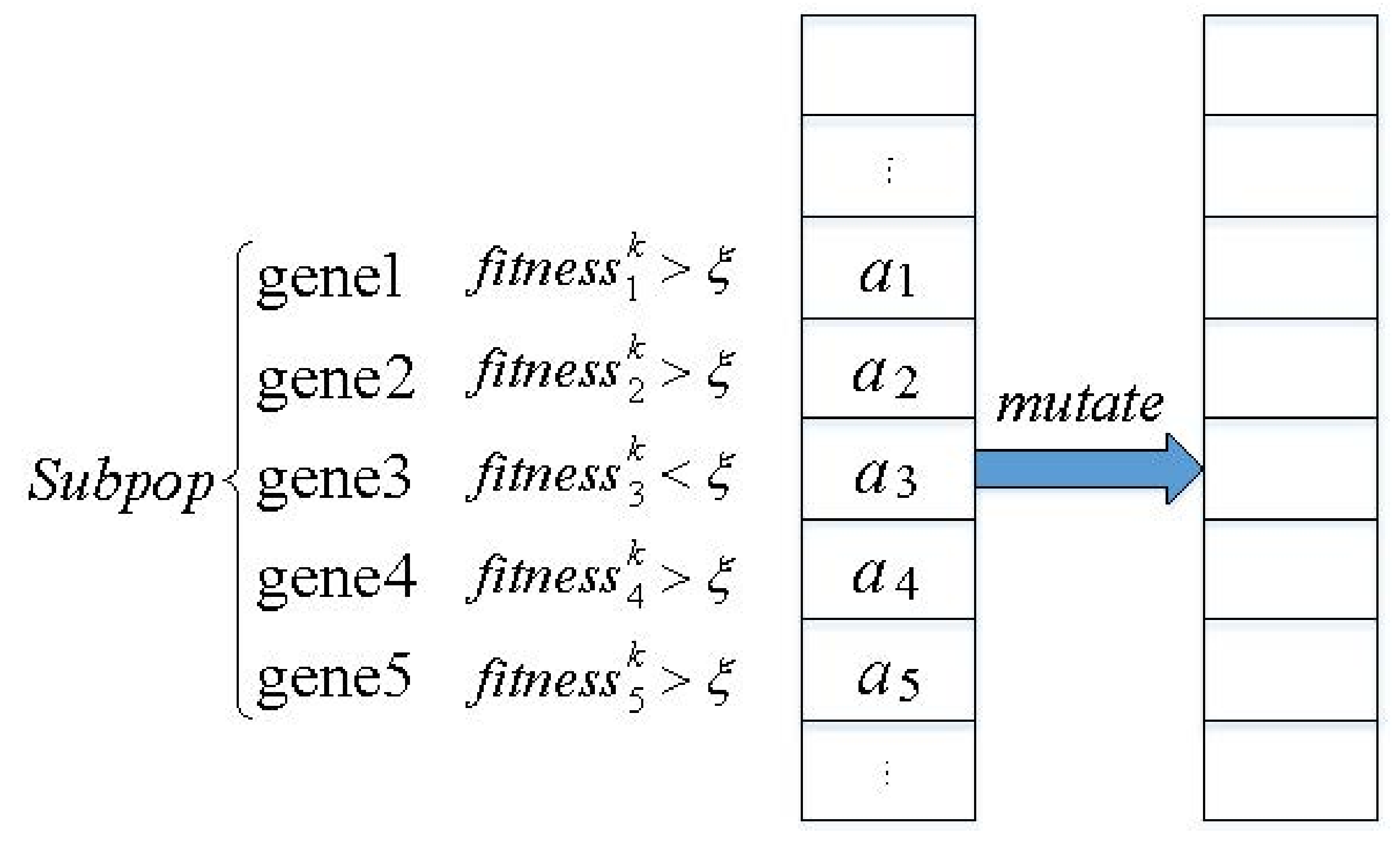
The rest parameters were set empirically. Among them, ${CP}_0=0.01$ [8]. Because we supposed that the superiority and inferiority of genes from different chromosomes were same, $\epsilon =0.5$. Moreover, in Equation (29), if ${CN}_j^k\ge 1$, then $\xi \le 0.5$. Therefore, in order to improve the efficiency of conflict resolution, we set $\xi =0.5$. The parameters were set as shown in Table 1.

Table 1. Parameter settings.

Model	Parameters	Description	Value
Upper level	${\sigma }_0^2$	Variance constraint	6
	$p_c$	Crossover rate of GA	0.9
	$p_m$	Mutation rate of GA	0.7
	$g_{\max }$	Maximum generations of GA	100
	$pop\_size$	Population size of GA	100
Lower level	${CP}_0$	Allowed conflict probability	0.01
	${\chi }_{GD}$	Ground delay cost weight	0.4
	${\chi }_{FA}$	Flight altitude shift cost weight	0.6
	$P_{GD}$	Ground delay probability	0.5
	$P_{FA}$	Flight altitude shift probability	0.5
	$\epsilon$	Linear recombination factor	0.5
	$\xi$	Expected local fitness	0.5
	$P_c$	Crossover rate of CCEA	0.8
	$P_m$	Mutation rate of CCEA	0.1
	$G_{\max }$	Maximum generations of CCEA	100
	$Pop\_size$	Population size of CCEA	100

5.3. Results Analysis

In the lower-level programming model, a CCEA based on CS was applied for the solution. The trends of the conflict number and the total flight time of the flights with the evolutionary generation are given in Figure 20. The conflict-free optimal trajectory is depicted in Figure 21.

Figure 20. The trends of the conflict number and the total flight time.

Figure 21. Conflict-free optimal trajectory.

It could be separated into two distinct stages based on the inflection point (red line) in the left picture. The number of conflicts in the first 60 generations progressively reduced to zero. The total flight time fluctuated continually between 1948.75 h and 2200.75 h. This was due to the existence of time-varying and altitude-varying wind in the process of conflict resolution. When the departure time and flight altitude were modified, the wind condition had great variability. However, in the stage of 60 to 100 generations, there were no longer any conflicts, and the algorithm solved for the shortest total flight time. Therefore, the total flight time in this stage was stably reduced until convergence.

In addition, the trend of the conflict number based on the random strategy is also given in the left picture (blue line). It is clear that the blue line converged slowly and could not reach a solution without conflict. As a result, the performance could be effectively enhanced by the heuristic strategy based on CS.

In order to analyze the advantages of the optimization results, the trajectory in structured airspace, the great circle trajectory, and the bi-level optimal trajectory were compared. The conflict number, total flight time, variance, and deviation were used as indicators to evaluate the safety, efficiency, and predictability, as shown in Table 2.

Table 2. The comparison between the trajectory in structured airspace, the great circle trajectory, and the bi-level optimal trajectory.

Indicators	Trajectory in Structured Airspace	Great Circle Trajectory	Bi-Level Optimal Trajectory
Conflict number	1672	1844	0
Total flight time (h)	2480.52	1869.75	2041.62
Variance (h2)	6.55	6.94	5.78
Deviation (h)	19.72	15.53	12.32

Notice that the bi-level optimal trajectory was greatly improved in terms of flight safety and predictability, as it was the only one without conflict. On the contrary, both the trajectory in structured airspace and the great circle trajectory had large numbers of conflicts. Due to the shortest distance, the great circle trajectory had the best performance in flight time. Comparing the trajectory in structured airspace with the bi-level optimal trajectory, the total flight time was reduced by 438.9 h, about 17.7%. For each flight, it was reduced by about 17.8 min. This was because, in structured airspace, aircraft must follow a planned route, as shown in Figure 17. Not only does this incur extra flight distance, but it also diminishes the flexibility of the aircraft. However, the bi-level optimal trajectory was more flexible and, thus, could effectively take more advantage of the predominant tailwinds. In addition, it allowed the aircraft to avoid areas with higher uncertainty (with a darker background color) and improve predictability while minimizing variance and deviation.

5.4. Time-Varying Wind Analysis

The analysis of time-varying wind enabled the characteristics of the wind to be effectively captured during the trajectory planning. Existing studies have usually supposed that the wind is constant during the whole flight operation process, which lacks a comprehensive perspective.

The optimal trajectory considering time-varying wind was compared with an optimal trajectory with constant wind. The forecast data from 8:00 a.m. to 9:00 a.m. was taken as the constant wind. After optimization with the bi-level programming model, the optimal trajectory with constant wind is shown in Figure 22. When it was analyzed with time-varying wind, the corresponding indicators were as shown in Table 3.

Figure 22. Optimal routes with constant wind.

Table 3. The comparison between optimal trajectories in constant wind and time-varying wind.

Indicators	Constant Wind	Time-Varying Wind
Conflict number	27	0
Total flight time (h)	2121.67	2041.62
Variance (h2)	6.24	5.78
Deviation (h)	11.96	12.32

It can be concluded that the optimal trajectory with constant wind mostly chose to avoid encountering strong headwinds in the northwest. Combined with Figure 18, notice that the wind tended to weaken. When the time-varying wind was not taken into account, the aircraft could not effectively obtain the wind information and decided to detour. In contrast, when we considered the time-varying wind, then the aircraft could make full use of the wind conditions according to the dynamic information.

A flight from Guangzhou, China (ZGGG), to Amsterdam, Netherlands (EHAM), was used for further analysis. The coordinates of the entry and exit points were $(105°18\prime \mathrm{E},28°29\prime \mathrm{N})$ and $(82°53\prime \mathrm{E},46°52\prime \mathrm{N})$, respectively.

The route of ZGGG–EHAM in the structured airspace (red), the optimal route with constant wind (green), the optimal route with time-varying wind (yellow), and the great circle route (black) are given in Figure 23. It can be seen that the green line was more northward. As already noted, the wind tended to weaken, and the wind uncertainty tended to strengthen continuously. In order to reduce the distance, the route with time-varying wind could choose a route that was closer to the great circle route. Conversely, the route could shift northwardly to avoid strong headwinds if the wind was constant all the time. Considering the real situation, the strong wind vanished when the aircraft arrived. Table 4 shows the comparison of the flight time, variance, and deviation of the optimal routes from ZGGG to EHAM.

Figure 23. Optimal routes from ZGGG to EHAM, structured airspace (red), great circle (black), constant wind (green), time-varying wind (yellow).

Table 4. The comparison between the routes from ZGGG to EHAM.

Indicators	Route in Structured Airspace	Great Circle Route	Route with Constant Wind	Route with Time-Varying Wind
Flight time (min)	232.81	196.55	214.34	205.42
Variance (min2)	8.42	9.68	6.94	5.71
Deviation (min)	13.71	14.66	10.29	9.68

5.5. Comparative Analysis with Two-Stage Model

In existing studies, two-stage models have often been developed for trajectory planning. To determine the optimal route, only flight efficiency is taken into account in the first stage. In the second stage, the model concentrates on strategic CD&R. However, the current optimal route changes if the departure time or flight altitude are changed, which reduces the operating efficiency due to time-varying and altitude-varying wind. The established bi-level programming model integrating efficiency and safety could continuously optimize the optimal route while ensuring safety.

Figure 24 shows the optimal route planned in the first stage with the conflict locations. Notice that the result of the first generation in the bi-level were the same, where the initial number of conflicts was 3841, and the conflicts were concentrated in the eastern airway dense area, containing continuous conflict between two aircraft.

Figure 24. Initial optimal route (red line) and initial conflict location (yellow dot).

The number of conflicts, total flight time, variance, deviation, and CPU time corresponding to the optimal solution obtained by the two-stage model are given in Table 5.

Table 5. The comparison between two-stage and bi-level optimal trajectory.

Model	Two-Stage Optimal Trajectory	Bi-Level Optimal Trajectory
Conflict number	72	0
Total flight time (h)	2255.74	2041.62
Variance (h2)	5.92	5.78
Deviation (h)	12.41	12.32
CPU time (s)	6994.81	7507.44

When compared to the bi-level programming model, the optimal trajectory obtained by the two-stage model was of worse quality. Conflicts still existed in the two-stage model, and the average flight time per aircraft was increased by 8.7 min, while the overall flight time was nearly 214 h longer. From the results of the conflict numbers, it can be concluded that the bi-level model indirectly added the strategy of modifying the shape, which is an important factor for acquiring a conflict-free solution. From the flight time analysis, we may infer that the bi-level model constantly adjusted the optimal route according to the latest flight plan and had an important advantage in multi-aircraft cooperative trajectory planning. Notice that there was no significant difference in the predictability of the trajectory between the two models, which indirectly proved the influence of time-varying wind on the predictability. The CPU time for the bi-level model was 7507.44 s, which was 513 s longer than the two-stage model. Undeniably, the proposed method increased the complexity of the problem, but it was acceptable.

Figure 25 shows the adjustment of the departure time and flight altitude corresponding to the optimal solutions of the two models. The two-stage model needed to make more adjustments to effectively resolve the potential conflicts, which was because the flight routes were unchangeable. However, the bi-level model indirectly added a conflict resolution method, allowing it to make fewer adjustments.

Figure 25. The adjustment of departure time and flight altitude corresponding to the optimal solutions of bi-level and two-stage models.

6. Conclusions and Future Work

We proposed a methodology for strategic trajectory planning in FRA considering time-varying and altitude-varying wind forecast uncertainty. Firstly, the effect of wind on trajectory prediction was introduced. Then, a bi-level programming model was established because of this impact, which resulted in the optimal route altering when the departure time and flight altitude were changed. The upper level of the model focused on flying effectiveness while attempting to reduce the total flight time. The lower level of the model minimized the number of conflicts and assured safety. The significance of taking time-varying and altitude-varying wind into account for trajectory planning was demonstrated by comparing the optimization results with the flight times of the trajectory in structured airspace and the optimal trajectory with constant wind. To verify the advantages of the proposed model, the results were compared with the optimal trajectory obtained by a two-stage model. The indicators suggested that the proposed method may improve flight efficiency while also successfully resolving conflicts between aircraft. Since the conflict resolution problem was a large-scale combinatorial optimization problem, a heuristic strategy based on CS was employed to speed up convergence. The algorithm comparison showed that such a strategy was effective.

In this study, the wind was a discrete random variable, but research is still required when the wind is a continuous random variable. Future work should focus on additional analyses of time-varying and altitude-varying wind. Meanwhile, only a single optimal trajectory was given in the upper-level planning; if a multi-objective optimization is introduced, it can provide diverse options for conflict resolution in the lower-level planning. In addition, considering a case of limited airspace can make trajectory planning more realistic.