4.1. Geostatistical Analysis and Spatial Distribution of PTEs
One of the characteristics of geostatistical methods is that the frequency distribution of the data should be close to a normal distribution. However, most applications are not represented using a normal distribution. This is caused by several factors such as the density and sampling scale, which may not be representative, and errors in the laboratory analysis. Therefore, it is necessary to transform the original data to normally distributed data [
56]. In soil contamination studies, geostatistical analyses are a powerful tool to separate sources contributing to observed pollution. This technique has been widely used to differentiate between different natural sources that cause variations in soil composition and to identify pollution sources affecting the content of pollutants in the soil [
62]. The main application of geostatistics to soil science has been the successful estimation and mapping of soil attributes in unsampled areas [
56,
62,
63]. In our study, the PTE data were processed through a geostatistical analysis to find the best parameters needed to conduct the spatial interpolations. The nuggets and variograms helped us represent the variation in the composition of the elements present in urban dust. In the case of the nugget effect, this refers to the situation in which the difference between measurements taken at sampling locations that are close together is not zero [
64]. Other air quality studies have estimated variograms and nuggets, suggesting the use of spherical models with a correlation coefficient greater than 0.90 [
18]. On the other hand, the models obtained in our analysis are summarized in
Table 5 and are consistent with other studies. For example, Zhang et al. (2014), Li and Feng (2012), and Duan et al. (2015) used multivariate and geostatistical analyses of PTEs found in soil samples, finding that linear, spherical, exponential, and Gaussian models can be fitted adequately to the data [
56,
62,
63]. The models may vary from each other depending on the number and density of samples (km
2/sample). A higher density and number of samples can significantly reduce errors and present more stable models [
52].
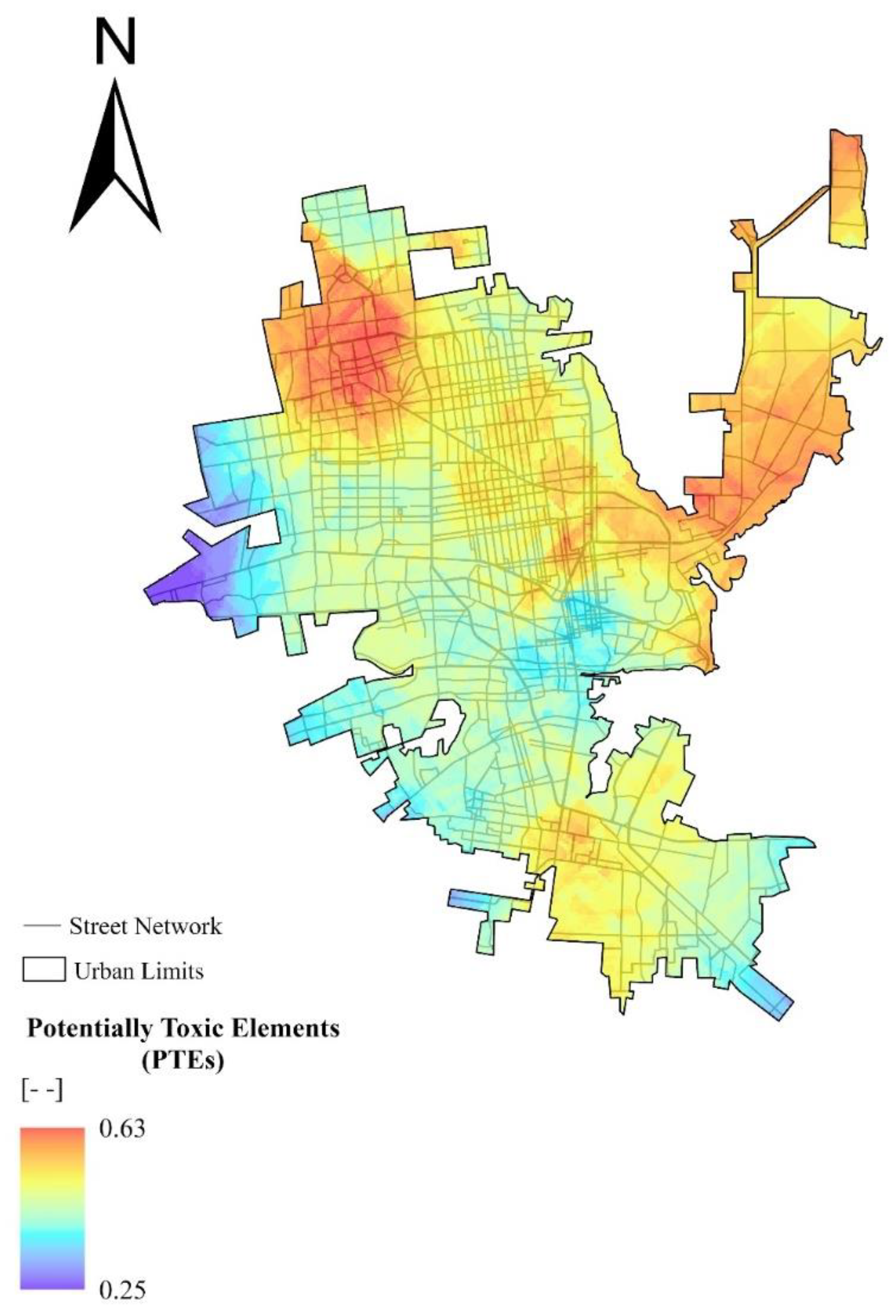
The spatial distribution of PTEs is a powerful indicator that allows by itself for one to identify areas vulnerable to the exposure of these elements. Different sources of pollutant emissions from domestic, commercial, and industrial activities can further concentrate some elements in certain parts of the city, such as Pb and V from combustion exhaust, industrial processes, coal combustion, metallurgic processes, and the construction industry [
6,
7,
65], or chromium (Cr) from traffic paint, which can be liberated by high temperatures and radiation or by the degradation of the asphaltic cover [
6].
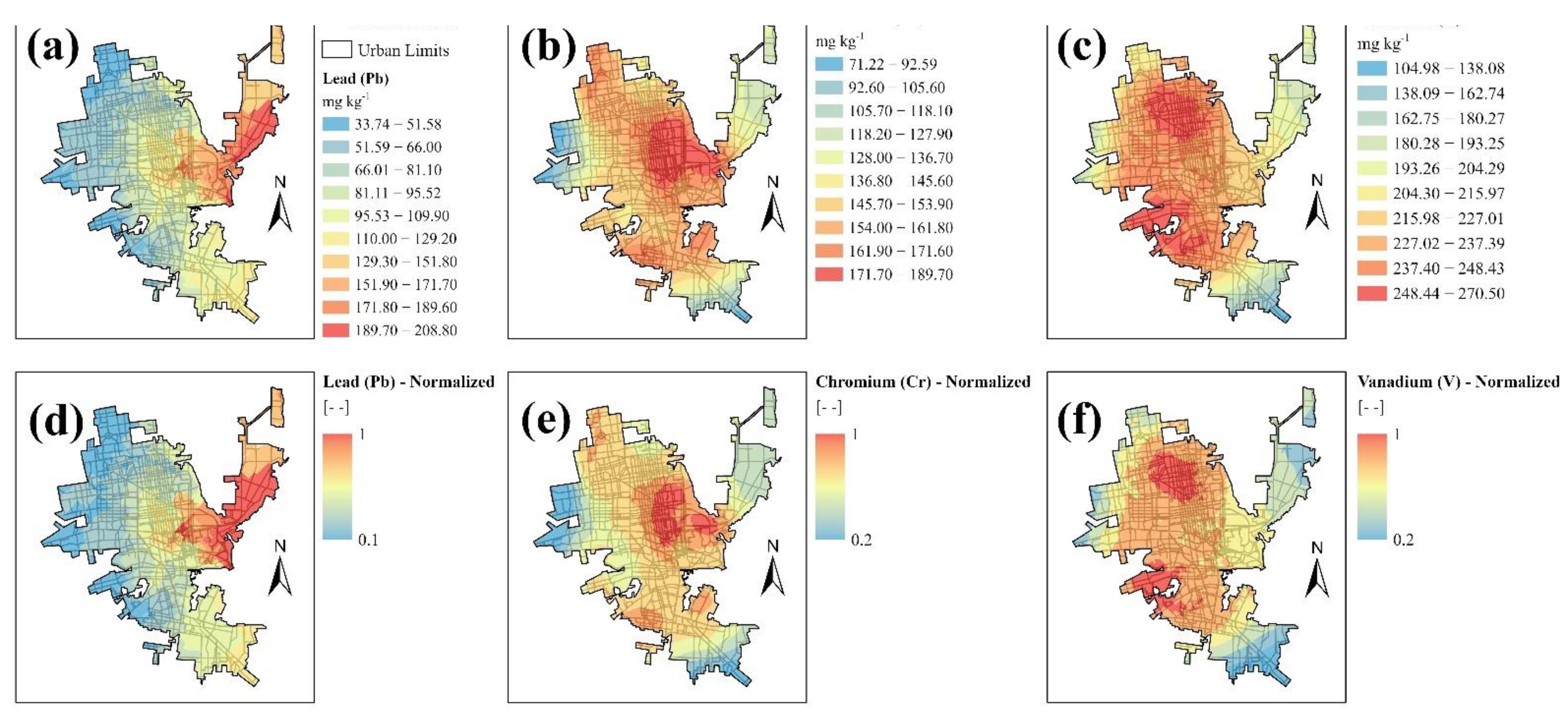
Meza-Figueroa et al. (2018) reported concentrations of Pb from 21.7 to 778.1 mg·kg
−1 in road dust that were consistent with our data range of 15.2 to 979.8 mg·kg
−1 [
6]. In the same way, the spatial distribution of Pb presented in their work is consistent with our Pb distribution map. On the other hand, Cr concentrations can be attributed to metal-based traffic paints on the streets and playground paints [
2,
6]. Traffic painting releases Cr particles due to the photodegradation process. It has been reported that fresh yellow traffic paint contains high concentrations of Pb and Cr [
6]. In this study, higher concentrations of Cr were found in the center of the city (
Figure 5b). This can be attributed to the high levels of vehicular traffic and the physical conditions of the asphalt and traffic paint. Meza-Figueroa et al. (2018) also measured the Cr concentrations in road dust in Hermosillo [
6]. The Cr concentrations reported in their work ranged from 112.7 to 257.5 mg·kg
−1, which coincide with our results of 112.6 to 273.5 mg·kg
−1. The spatial distribution map presented by Meza-Figueroa et al. (2018) is consistent with our distribution map of Cr in Hermosillo.
Vanadium is a toxic metal, which if inhaled can induce pulmonary tumors and increase the probability of lung cancer [
61]. The concentrations of V in the ambient air vary widely between rural and urban areas [
65]. In urban areas, the V is strategically important due to its wide use in fossil fuels, steel manufacturing, aircrafts, and cement plants [
60,
61,
66]. This could explain the large V distribution in
Figure 5c in Hermosillo. Li et al. (2020) measured V in samples of farmland soil in China and the average content reported was 121 mg·kg
−1 [
61]. Our results compared with Li et al. (2020) show higher concentrations with an average of 242.1 mg·kg
−1. This is mainly due to the difference in climates, whereby Hermosillo, being a semiarid city, tends to accumulate more elements in urban dust.
4.2. Hot Spots
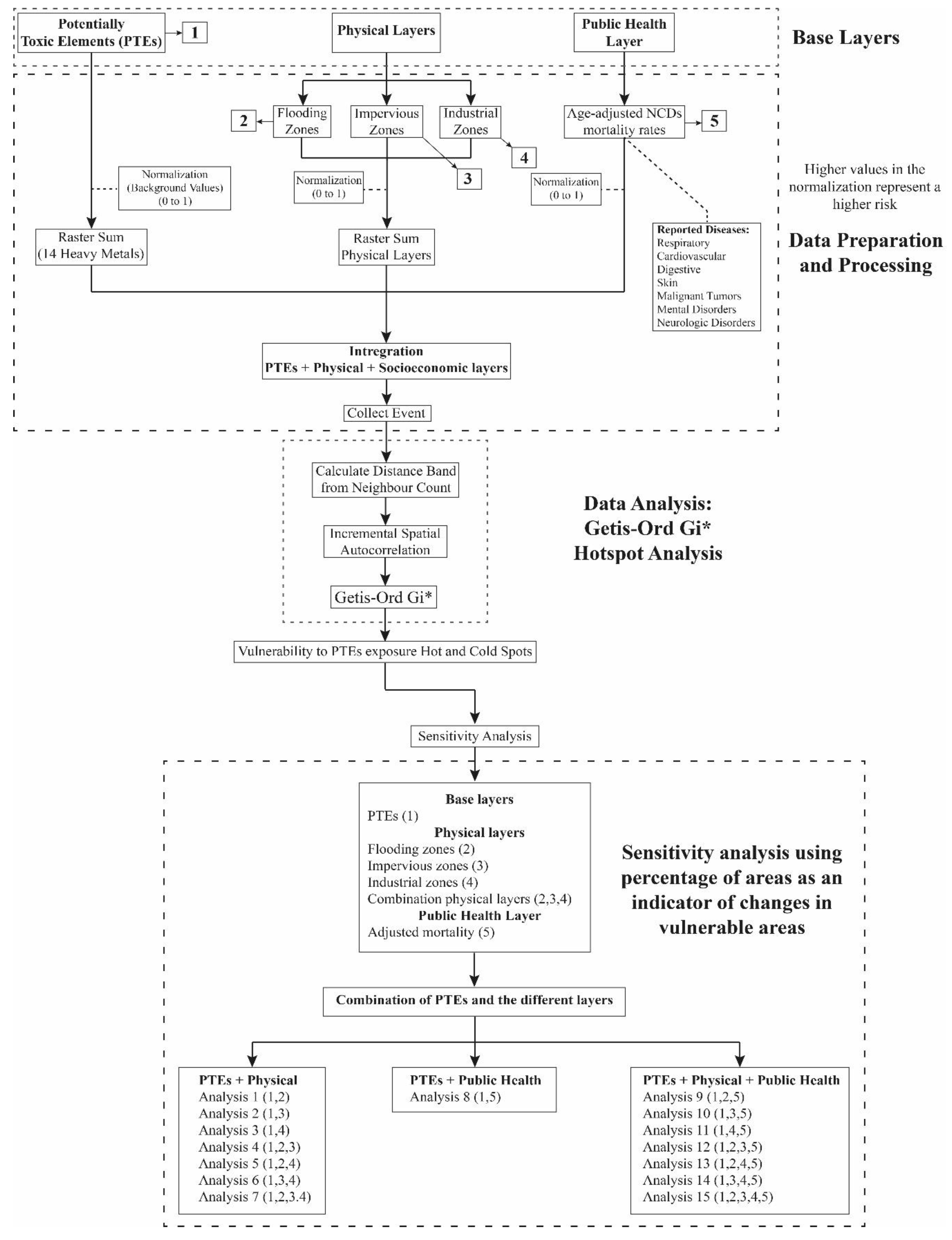
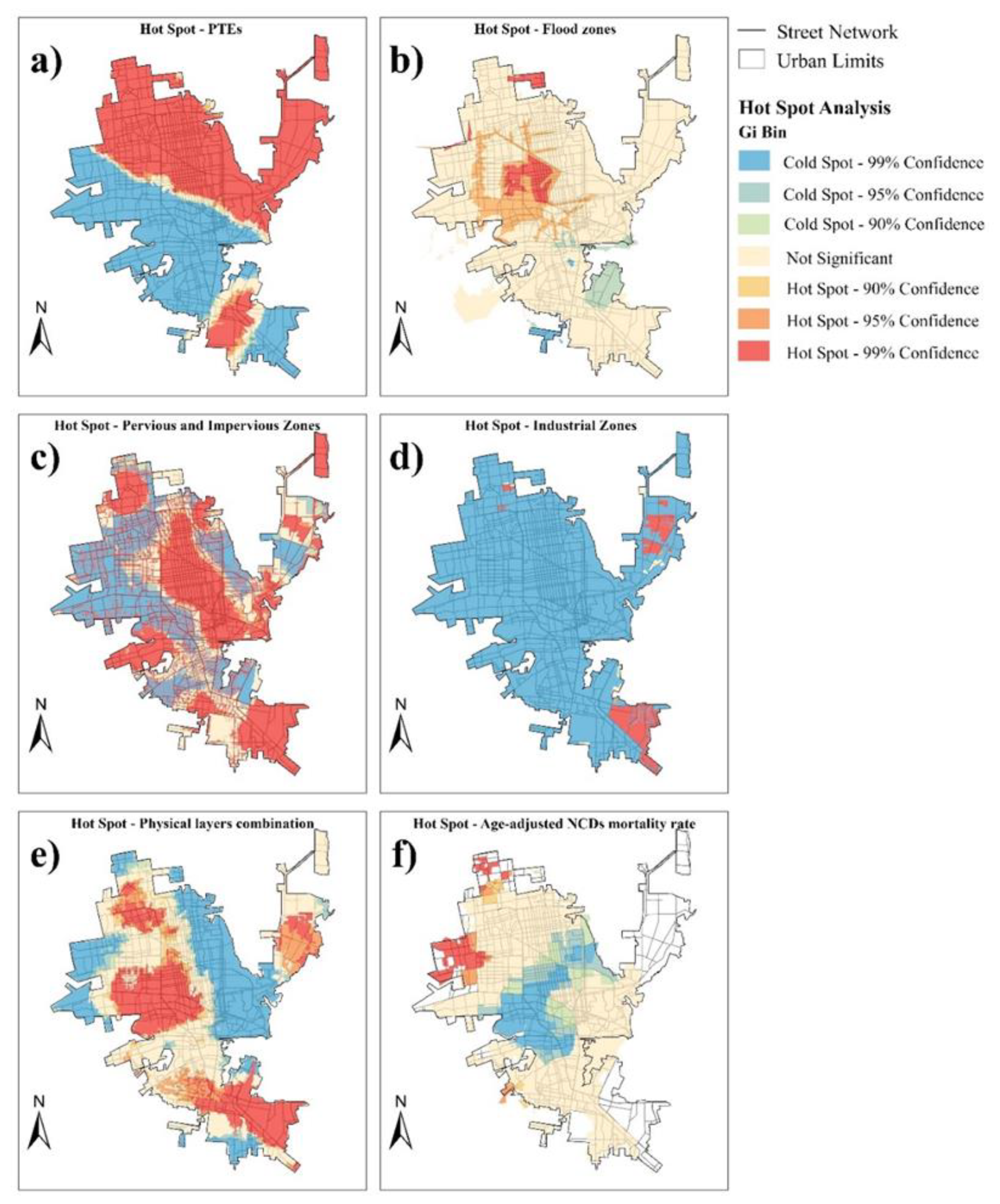
Our hot spot results show the spatial distribution of the vulnerability for the different analyses in Hermosillo. In the case of flooding,
Figure 7b shows these areas in the center of the city. The vulnerability levels in those areas that have zero or almost zero soil permeability, such as streets, commercial and industrial areas, and highly inhabited areas, are displayed in
Figure 7c. On the other hand,
Figure 7d shows where the medium- and high-risk industries have an important influence on the vulnerability due to the productive activities that result in the emission of pollutants into the atmosphere. The integration of all physical layers can be observed in
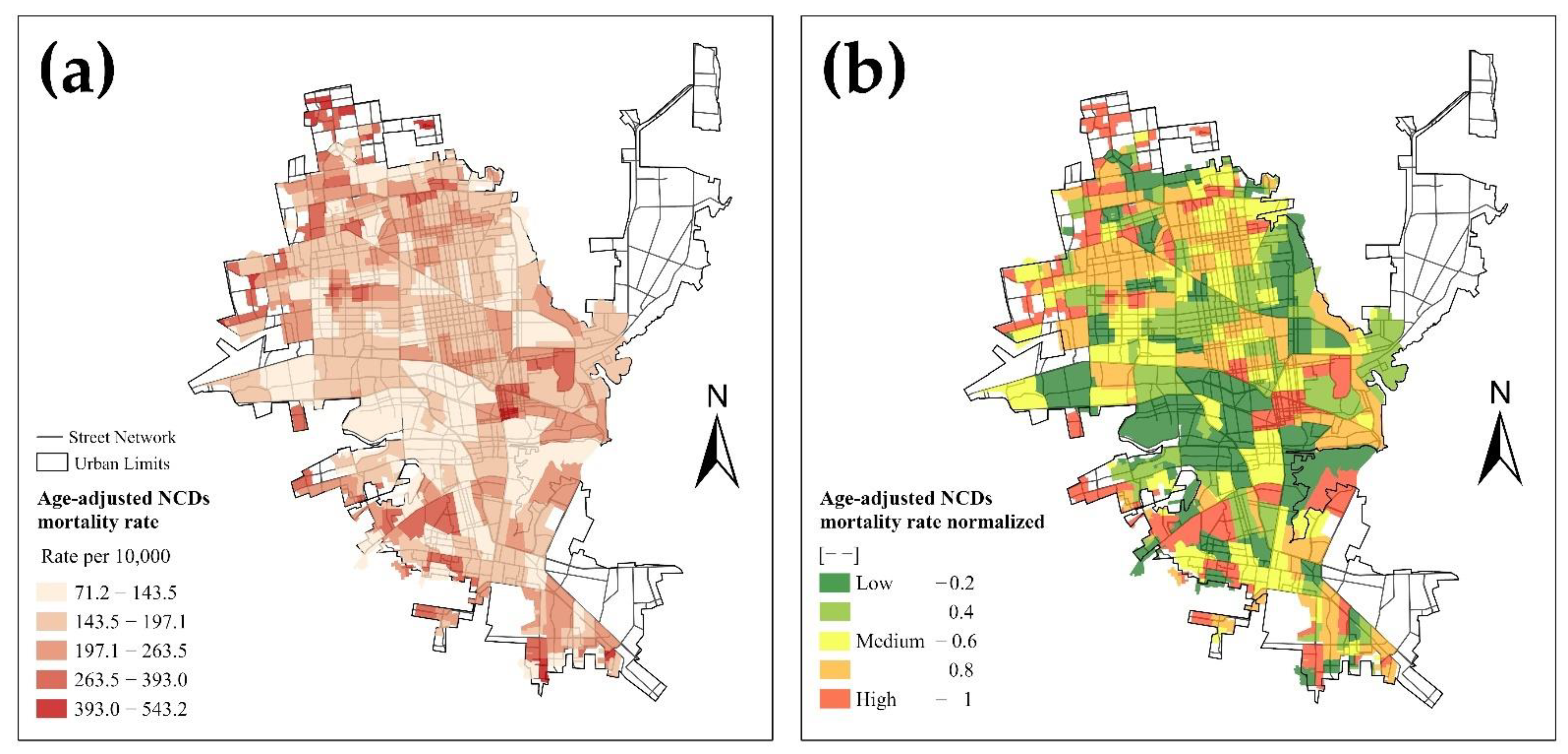
Figure 7e, where areas of greater vulnerability are present in those areas that all layers coincide. Finally, a hot spot was mapped for the age-adjusted NCD mortality rate in
Figure 7f, where in the north and northwest of the city a higher risk of deaths associated with non-communicable diseases can be observed.
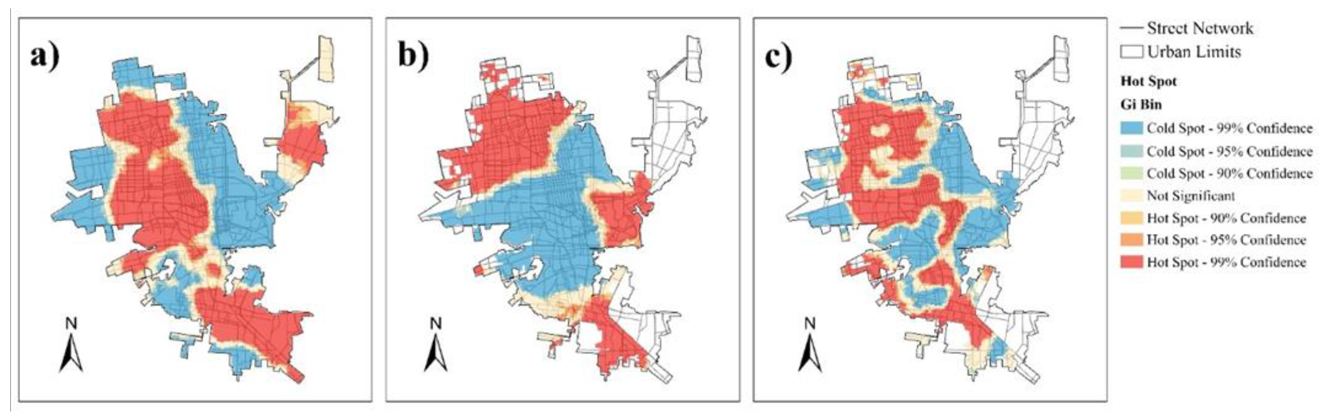
Figure 8 shows the vulnerability to PTE exposure when integrating physical and public health variables.
Figure 8a shows the combination of PTEs, flood zones, pervious and impervious zones, and industrial zones. The streets and highly populated areas in Hermosillo have a great influence on the accumulation and transportation of PTEs found in dust. This causes a high vulnerability in those areas that present floods during rain events, influenced by the low or null permeability of the soil.
Figure 8b is the result of the combination of the PTEs and the age-adjusted NCD mortality rate. The vulnerability areas coincide with those areas (west and northwest) where high concentrations of PTEs have been registered, as well as those areas with the highest incidence of mortality that could be associated with the exposure of PTEs.
Figure 8c is one of the most important figures obtained due to its representation of the combination of all variables (PTEs, flood zones, pervious and impervious zones, industrial zones, and the age-adjusted NCD mortality rate). In this case, the areas of greatest vulnerability coincide with those areas where there is a great impact by floods influenced by impervious areas in the city. The transport of urban dust and PTEs during flood events is consistent with the spatial distribution of the PTEs and the areas where deaths that could be related to PTE exposure have been reported.
In the same way as in this work, Navarro-Estupiñan et al. (2020) also used percentage metrics to identify areas vulnerable to heat risk in Hermosillo, Mexico [
39]. Zones with high vulnerability were identified in the center of the city, where the hot spots ranged from 1.92 to 36.16% for low- and medium-density housing and mixed areas. Towards the periphery of the city in northern, western, and southern areas, zones with low vulnerability (cold spots) were identified containing high- and medium-density housing, mixed areas, and housing reserves, ranging from 2.22 to 3.10%. Considering the population percentages of Hermosillo in 2010, based on their results the authors suggested that 16.6% live in areas of high vulnerability, 13.9% in areas of medium vulnerability, and 70.4% in areas of low vulnerability.
4.3. Sensitivity Analysis
Once the hot spot maps were obtained, the sensitivity analysis was conducted to identify the layers (variables) with the greatest influence on the spatial distribution of cold and hot spots.
Table 6 shows the vulnerable areas considering each variable individually, except for the analysis where the flood zones, pervious and impervious zones, and industrial zones were combined. On the other hand,
Table 7 shows the different combinations between the PTEs, physical maps, and public health maps.
The floods and pervious and impervious zones were the variables that most affected the spatial distribution of the hot spots. The hot spot base map (PTEs) at 99% confidence represented 48.8% of the total area. Analysis 3, where the floods and pervious and impervious zones were not used, decreased to 31.8%. Secondly, in analysis 6, where the flood zones were not used, the 99% confidence areas decreased to 24.9%. Therefore, the integration of these variables has a significant influence on the spatial distribution of vulnerable areas.
Analysis 7 shows the combination of the spatial distribution of PTEs and the physical layers, where the hot spot at 99% confidence represents 41.3% of the total area. In analysis 6, where only flood areas are not considered, the area representing hot spots decreases from 41.3% to 24.9%. Therefore, the flood zones were the most sensitive variable due to the weight they had during binary normalization. The combination of the PTEs and the age-adjusted NCD mortality rate can be observed in analysis 8, where the hot spot at 99% confidence represents 40.0% of the total area. Finally, analysis 15 shows the combination of PTEs, physical maps, and the public health layers, where the hot spot at 99% confidence represents 35.9% of the total area. In analyses 9 and 13, where only the permeable and impermeable areas were not considered, the area representing the hot spots decreased from 35.9% to 30.1% and 29.5%, respectively. This means that the permeable and impermeable zones were the most sensitive variables due to the weight they have in the spatial distribution.
Several studies that have tested single and multiple variables using clustering techniques, particularly using the Getis-Ord G
i* tool, have reported the use of sensitivity analyses to demonstrate the influence of different variables in their studies. McClintock (2012) performed multiple comparison tests (
z-scores) in a hot spot analysis to identify soil lead contamination at multiple scales in Oakland, California [
35]. This author used land use data, soil Pb concentrations from 112 sites (ranged from 3 to 979 mg·kg
−1), types of vegetation, and variations in geographical zones (neighborhood-scale) to evaluate the risk of Pb contamination. In this study, a range of
z-scores from −2.58 to 2.58 was found, where a high
z-score indicates the clustering of high soil Pb concentrations, while a low
z-score indicates the spatial clustering of low Pb concentrations. Median
z-scores suggest that there is no significant spatial relationship between the Pb concentrations and the geographical zones. A Getis Ord G
i* test on the neighborhoods-scale data revealed the significant clustering (hot spot) of elevated Pb concentrations in the southwest corner of West Oakland. Similarly, Lee and Khattak (2019) used
z-scores and
p-values to determine differences in spatial clusters or hot spot areas of crash points on roadway networks in Lincoln, Nebraska [
34]. Eight high-severity crash clusters and six low-severity clusters were identified in the study area. The clusters were determined based on the number of statistically significant crash points (at least eight points in a cluster) and their significance level (
p ≤ 0.01).
Cooper-Vince et al. (2018) used
p-values (Poisson regression) to identify the risk of depression associated with water insecurity, gender, marital status, education, assets of wealth, and overall health using a hot spot analysis in a rural parish in Mbarara District, Uganda [
37]. The results of the sensitive analysis suggest that women who reside in a water insecurity hot spot have a 70% higher risk (
p = 0.003) of probable depression compared with women who do not reside in a water insecurity hot spot. On the other hand, men who reside in a water insecurity hot spot do not have a risk of probable depression (
p = 0.92); however, with the multiple regression model, the interaction between gender (men and women) and living in a water insecurity hot spot was not statistically significant (
p = 0.08). The results of the sensitivity analysis suggest that education level, age, marital status, wealth, and general health are not significant factors in depression. In this case, gender (female) and areas of water insecurity were the most important factors in determining depression.
The sensitivity analysis carried out by García et al. (2018) to evaluate water infrastructure failures in three cities in California used multivariate linear regression models (
p-values) to determine significant differences between different variables (the pipe material, season, diameter, and soil types) and across the cities [
67]. The sensitivity analysis suggested that the selected pipe material, season, diameter, and soil types have statistically significant (
p ˂ 0.05) effects on the pipe longevity.
Another study conducted by Zhang and Tripathi (2018) used a Pearson correlation (
p-value) in a hot spot analysis to investigate lung cancer and its spatial correlation to mortality and fine particulate matter (PM
2.
5) using data from 2008 to 2012 [
38]. In this case, the age-standardized incidence rate (ASR) and age-standardized mortality rate (ASMR) of lung cancer were closely correlated with the PM
2.
5 value (
p ≤ 0.01). A second correlation was performed to determine the correlations between lung cancer, PM
2.
5, wind speed, and wind direction. The results suggested that the wind direction is an important factor that affects the PM
2.
5 value (
p ≤ 0.01).
Finally, Navarro-Estupiñan et al. (2020) performed a sensitive metric analysis (%) using thermal maps, socioeconomic data (i.e., gender, age, marital status, education level, health services), and physical indicators (housing with electricity, fridge and washing machine, Internet access, and phone and cellphone, as well as impervious areas and streets) to determine the differences in hot spot areas in different analyses compared with the hot spot map with the analysis of all indicators in a semiarid city in Northwestern Mexico [
39]. The most sensitive indicators were found to be age and education (≥15 years old without elementary school), with a 2.0% difference in hot spot areas, followed by health (without health public service) at a 1.6% difference and age (18–65 years) at a 1.1% difference. These indicators are related to heat exposure through outdoor activities such as construction works and agricultural activities in which people participate daily for economic reasons. Although the results presented by Navarro-Estupiñan et al. (2020) do not evaluate the same variables as in our study, their results can be compared in terms of the units [
39]. The work proposed by Navarro-Estupiñan et al. (2020) determined the differences in the percentages of areas presented in the different analyses, such as for age and education and health and age [
39]. Our results in the same way determined the most sensitive variables in the distribution of vulnerable areas, as in the case of flood zones and permeable and impermeable zones (analysis 3) with a difference of 17% in more vulnerable areas. In the specific case of flooded zones (analysis 6), this variable showed a difference of 23.9%, being the most sensitive compared with the base map (PTEs).
The results presented in this work are not directly comparable to the other studies because all have different contexts, with the exception of the work conducted by Navarro-Estupiñan et al. (2020) [
39]. In our study, we were able to highlight the most dynamic variables after they were grouped with variables that do not change much over time. This procedure helped identify a more robust measure of vulnerability to PTEs. We argue that it is critical to conduct a sensitivity analysis to quantify the influences of different layers. Previous studies used statistical tools to highlight the influence of the variables used in their studies, which are valid tools that demonstrate the sensitivity of their variables. However, in our case, we quantified the spatial distribution changes in the final maps of vulnerability. We believe that this quantifiable spatial analysis of the increase or decrease in cold and hot spots provides a clearer picture of the most sensitive variables in terms of the influence on the overall vulnerability.


 ,
, 


