1. Introduction
The quality and quantity of raw materials play an important role in the manufacturing of steel production. Iron ore is the main raw material required in steel manufacturing. The management of steel industries thus needs to receive a consistent grade of iron with less variation. The raw material supplied to the plant must be uniform or within permissible limits of variation with the desired quantity. To supply the desired quality and quantity of raw materials to the steel plant consistently, the iron mine needs to prepare a robust mine plan. The majority of the existing computer-aided design solutions are built on the principle that the planning and scheduling of exploitation requires the combination of a significant quantity of various geological, operational, or economic data. The boundaries of each individual exploitation field, the sequence in which they should be carried out, as well as the locations of the access and preparation excavations, are decided throughout the production planning and scheduling phase [
1].
Production scheduling is an important and challenging issue in mine planning. The production scheduling method begins with the assumption of the initial production capacity of the mining system as well as estimates of associated costs and commodity prices. In this problem, the deposit is represented as a three-dimensional array of blocks. For each block, weight and metal content were estimated using information obtained from the borehole. In order to recover the metal in the form of either steel or raw iron, the block is first extracted from the ground and then treated in the plant. The revenue is generated after selling the metal to the market. The costs associated to produce metal include processing the raw materials in the process plant, mining the raw materials from the near- or sub-surface, and some auxiliary cost for selling the metals. The profit can only be made when the revenue generated from a mining block is higher than the total cost. It is noted that some mining blocks give positive and some blocks give negative profit (loss). In general, the cost of mining and the cost of processing are the same for all blocks (with some exceptions of processing cost varies with materials type). The major contributor to profit is the revenue, and revenue is highly dependent on the quality of the raw materials. The quality of a mining block is represented by grade, and the high-grade blocks generate higher revenue and thus produce more profit, and the low-grade blocks generate less revenue and thus incur a loss to the company. Therefore, the goal of a mining company is to produce as many high-grade blocks as possible, leaving low-grade blocks (which make a loss) in the ground. Moreover, due to the time value of money, the goal of a mining company is to generate more revenue in the early stages of the process. The mine production scheduling involves determining which blocks are to be mined during each lifecycle of the mine in order to maximize the net present value of the mining operation. Moreover, the production schedule must ensure the continuous operation of the plant which meets the production goals. The optimization for mine production scheduling can be accomplished by traditional (or conventional) and stochastic methods. Traditional methods of mining planning and mine optimization are considered single-estimated orebody models, and their calculations are ignore the uncertainty associated with the spatial distribution of the grade [
2,
3]. The basic assumptions of these models reflect the constant and real economic value of inputs derived from geological (estimated grade or metal content) and economic (metal price and cost) parameters. Ignoring any kind of uncertainty is a common weakness in mine production scheduling algorithms, which leads to the creation of unrealistic plans in terms of operational requirements [
4]. Dimitrakopoulos divides the uncertainty of the mining project into three main sources: geological, technological, and economic uncertainty [
5].
Neglecting geological uncertainty may lead to suboptimal production scheduling with significant deviations from production targets. The incorporation of geological uncertainty into open-pit mine planning is emphasized in [
2,
6,
7]. Ore grade uncertainty is considered to be a key source of risk affecting mining activity. Case studies have shown that integrating geological uncertainty in open-pit mine planning significantly reduces the risk of deviating from production targets and can increase project value by 26–28% [
8,
9]. Researchers have shown the importance of minimizing the deviations from the production targets while maximizing the discounted cash flow under geological uncertainty [
10,
11,
12]. The upside potential can be maximized and the downside can be minimized by a production schedule generated after incorporating the geological uncertainty [
7]. A multistage approach is proposed by Boland et al. [
13] to incorporate geological uncertainty in the production plan. A Monte Carlo simulation-based model is proposed by Groeneveld and Topal for mine design under uncertainty [
14]. Kumral [
15] proposed chance constraint-based production scheduling algorithm to incorporate mining uncertainty in the production plan. Asad and Dimitrakopoulos [
16] designed a mine plan under uncertain supply and demand using the Lagrangian relaxation of maximum flow algorithm. Researchers also proposed different a metaheuristic algorithm for stochastic optimization, including Tabu search, simulated annealing, particle swarm optimizer, etc., [
17,
18,
19].
The typical metal mine open-pit production scheduling formulation was taken into consideration as the solution approach for stochastic production scheduling under geological uncertainty. Assigning mining blocks to different production periods in order to maximize profit over the mine life and minimizing deviation from targets is the objective purpose of open-pit stochastic production scheduling. Multiple simulated orebody models are needed for the stochastic mine production schedule, which increases the number of decision factors, constraints, and demands a large amount of calculation time. It is typically impossible to optimally address the stochastic production scheduling of industrial-scale mining problems. The goal of this research is to create an algorithm that aids in real-world issue solving in a reasonable period of computational time with the closest possible solution. This paper presents a case study that focuses on the long-term production planning of an open-pit iron ore mine in India. The stochastic production scheduling was performed. For stochastic modelling, only the geological uncertainty or risk was considered; however, any other uncertainty can be incorporated with the additional computational burden. Two different solution strategies were considered for this case study: (a) sequential parametric maximum flow with repair branch and cut is proposed; (b) sequential branch and cut with the longest path algorithm, as proposed by Lamghari and Dimitrakopoulos [
20].
2. Description of Iron Ore Mine
The study was carried out at an iron ore mine in Central India. Due to the confidentiality agreement with the mining company, the name of the mine and name of the company were not disclosed here. These iron deposits are associated with rocks known to contain high-grade ores (hematite) and banded iron ores. These rocks form a narrow, highly dissecting, and discontinuous mountain range. The area belongs to the Indian Terrain Survey 64 H/2. The mining area of this study mine currently extends to 220.42 hectares. The mine is located in a hilly terrene. The ground level is located at 425 mRL, and the peak of the old bench is at 543 mRL. The drainage of the area is controlled by natural drainage channels and cutting across the hills. The total geology impact is in the east–west direction, with N to N–E having a varying dip angle of 40 to 60 degrees. The resistance of the iron ore in the outcrops in the general peneplane forms distinct hills and ridges, producing a saddle-shaped topography. The iron deposits are related to the banded iron form (BIF). The lithology in this area is predominantly sedimentary metamorphic. Hard blocks and abrasive banded hematite quartz (BHQ) and soft rock/shale form the lower wall and the hanging wall, respectively. Iron ore is very rich in the upper strata, and it is hard and huge in nature, gradually softening in depth. Geologically, the deposit has four types of iron ores: (a) massive hematite ore (Fe content = 65–67%); (b) compact laminated ore; (c) soft laminated ore; (d) lateritic ore. The mine covered by this lease is a fully established open cast echanized mine with a 3.5 MTPA ore extraction capacity. There is a 2:1 stripping ratio. Moreover, 4.6 cu. M. electric rope shovels, 5.5 cu. M. hydraulic shovels, and 50 T capacity rear dump BEML/HM dumpers are used in the excavation process in a traditional shovel–dumper combination. Currently, ore is delivered straight to a crusher that is nearby. At the rated capacity of 3.5 MTPA of ore, it is projected that 662 people are needed, although 753 people are already on site. At present, the mines is operated in three shifts for 310 days in a year. Drilling and blasting, loading and unloading, and mining excavation are the main activities that cause fugitive dust to be released into the air. As a result, there is no expectation of significant dust emissions or air pollution. There is an efficient mechanism for dust suppression. The operation of shovels, dumpers, dozers, and other transport vehicles will produce emissions, which will be routinely monitored and maintained to keep the emission below TLV. Topsoil will be placed separately and used for the regrowth of plants, while waste produced during the mining process will be used for backfilling and stacked in a systematic manner.
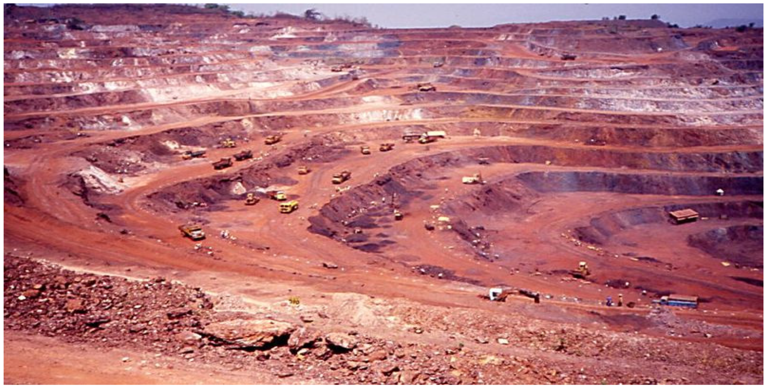
Groundwater occurs at about 430 mRL. The average amount of dewatering (based on the pump average) was about 1050 cum/day. Due to MMR-108 limitation, no mining is carried out below 443 mRL. All benches in the ore and waste are kept 10 m high and 20 m width for operating benches. In the footwall area, benches 483 and above and 473 (not including the west side) have been pushed to their ultimate pit positions. In the high wall region, 503 and 513 benches are in their final pit positions. Sleeping benches, 453 to 573 mRL, are excavated after the upper limit has been reached. The existing pit bottom is 418 mRL and the storage tank is 418 mRL. The pictorial view of the case study open-pit mine is shown in
Figure 1.
The ore-processing plant at case study mine involves three levels, and stage crushing and screening are used to produce BF-grade blocks and sinter-grade fines. The sediments show characteristics of low to medium grade ores, which include hematite and goethite as minerals and quartz, and pseudo-ores and iron clays as gangue minerals. The ore mineral distribution is about 28% overall, and the total area of gangue mineral distribution is about 72%. The main ore is hematite, with an area of 20%, of which about 6% of the grain is in a free state and the remaining 14% of the grain is not released. About 7% of the non-released particles can be released at 20-micron size. The remaining particle size is less than 15 microns. Goethite accounts for about 10% of the total area. All goethite particles are less than 30 microns in size, with about 2% of the particles in a free state and the remaining 8% of the particles not liberated. All undissociated particle sizes are less than 20 microns.
The area is characterized by a tropical climate and heavy rain from June to September. Except for a few rainy months, the remaining months are sunny with almost no rain. Meteorological data includes air temperature: maximum 47 °C, minimum 6.3 °C, with average 35 °C; the winter and summer average temperature are 14 °C and 27 °C, respectively. Regarding rainfall, maximum, minimum, and average values are 2088 mm, 1344 mm, and 660 mm, respectively.
The only attribute that was used in this study is Fe%. The mine authority only records this attribute from the borehole because the iron produced from this mine is of a very high grade, and there are very little impurities present in the ore. The geotechnical study of the deposit proposed a safe bench height of 10 m and a safe bench slope angle of 45°. All boreholes are drilled in a vertical direction.
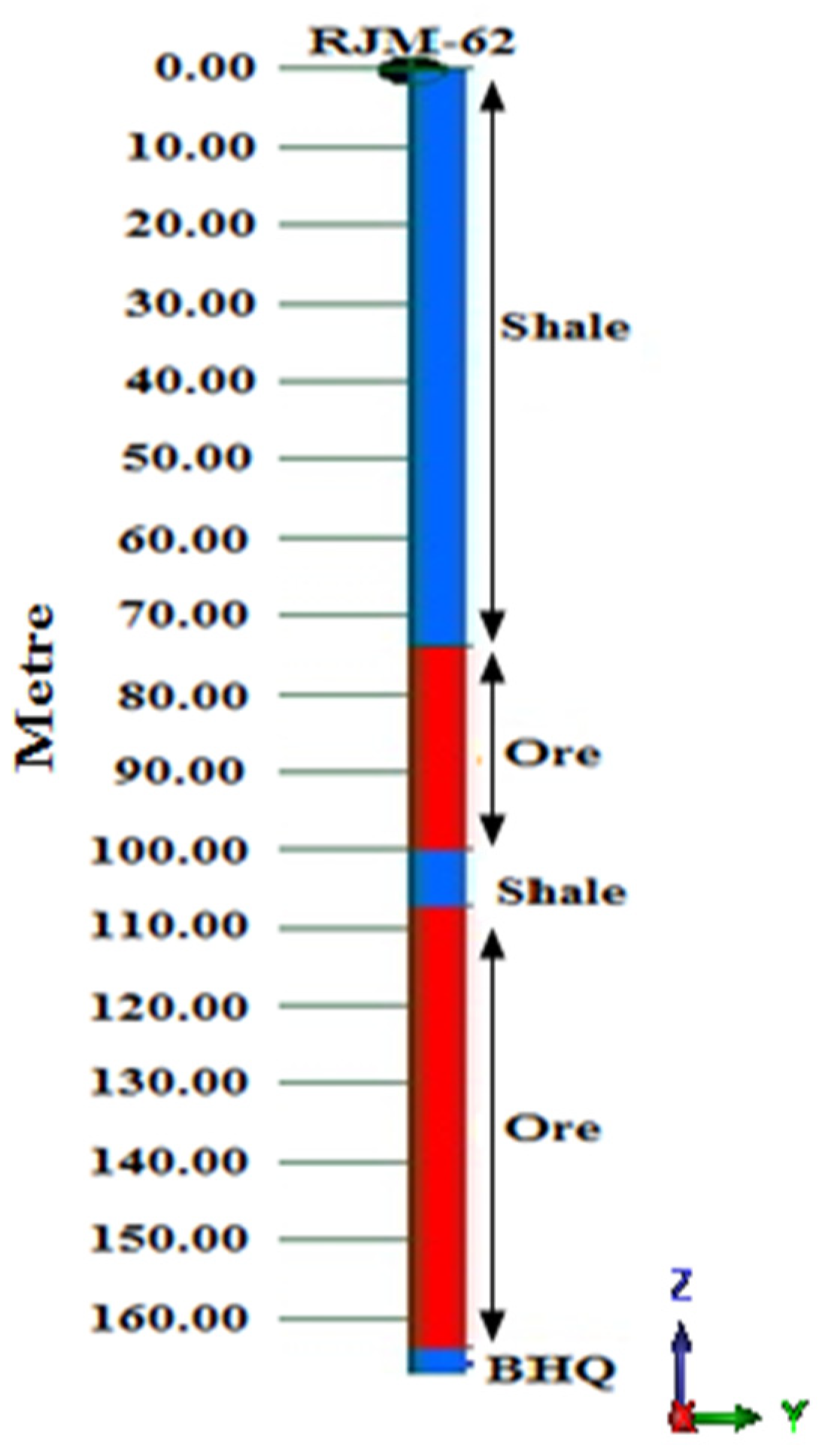
Figure 2 presents a borehole map with down-the-hole rock types. The assay data was composited at 10 m intervals for resource modelling of the deposit.
Figure 3 presents the composited point data with their associated assay value within the deposit.
3. Mathematical Model of Stochastic Mine Production Scheduling
The case study mine’s stochastic framework design for mine production scheduling is as follows: A decision variable
connected with a mining block of an open-pit mine, where
and
is the set of blocks. The scheduling of open-pit mine can be expressed as stochastic mixed integer programming with time indexed binary variables
which are defined by
if mining block is extracted at time
and
otherwise. The stochastic model’s goal is to maximize profit for all simulations
by allocating
blocks in
production periods and reducing deviation from production targets.
Subject to
Reserve constraints: The total number of blocks that can be mined is equal to Equation (2).
Slope constraints: First, we have to extract the overlying blocks before its predecessors.
Mining constraints: The maximum and minimum capacity to extract the materials from mine. In this process, the violation of this constraints is also not acceptable.
Processing constraints: The processing constraints with allowable violations are the plant’s production capacity and the minimum production requirement; these upper and lower bounds are necessary to ensure a smooth feed of ore to the mill; however, when the upper or lower limit bounds are exceeded, penalties are added to the objective function.
Metal production constraints: Metal production constraints, as with processing constraints, are allowed to deviate from their intended boundaries to some extent, and their related penalty terms are included in the objective function. The limits on metal production are presented as follows:
are the first stage decision variables. The deviation variables that contain simulation function are the second stage decision variables and depend on the realization of the uncertainty and values of the first stage decision variables.
where
4. Descriptive Statistics and Spatial Modelling
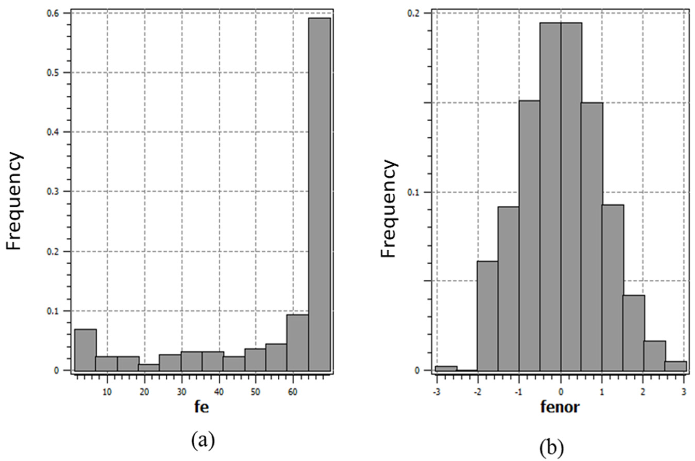
The exploratory data analysis was performed with the composited data set before resource modelling. For resource evaluation purposes, a total of 854 composited data were provided. The descriptive statistics of the composited data show that the iron grade is heavily skewed to the right, with significantly high variance. The frequency distribution of the data set was also prepared using the histogram plot (
Figure 4a). The histogram clearly shows the skewness property of the data set. It is seen from the descriptive statistics that the average grade of Fe is 54.9 (%) and the variance is 427.8 (%)
2. The K–S goodness of fit test was carried out for the normality checking of the data at 5% level of significance. The result of the K–S test shows that the data are not normally distributed.
The sequential Gaussian simulation (SGS) was used for the resource modelling of the deposit [
21]. The SGS needs the data to be normally distributed. The statistical analysis of the data set already revealed that they were not normally distributed. Therefore, it was obvious to transform the data with some mapping function. The transformed data were then used for modelling the variogram to measure the spatial variability of the deposit.
Figure 4b shows the histogram of normal score-transformed data. From the visual observation of the histogram, the data are evidently normally distributed. The K–S test confirmed the normality of the transformed data set. From the descriptive statistics of the normal score data, the mean is 0 and the variance is very close to 1, both of which are necessary for the SGS method.
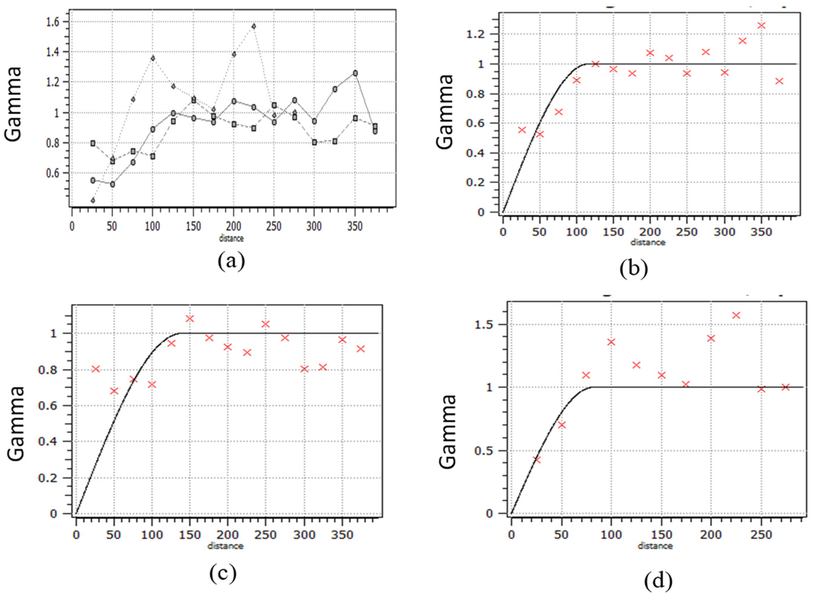
The deposit’s directional experimental variograms were estimated in two separate directions, namely 0 and 90°, with a spread of 45°. The variograms along strike were calculated with 25 m lag spacing. Variograms were also calculated in the downhole direction (−90° dip). The presence of anisotropy was demonstrated by the directed variograms. Spherical variogram models were used to suit all of the variograms. A single structure with a nugget model was used to fit all of the variograms.
Figure 5 shows directional variograms for both the experimental and fitted theoretical models.
The variogram model parameters and the normal score-transformed composited data were then used to generate 20 simulated realizations of the deposit. The simulation realizations were then back transformed to obtain the simulated map in the actual domain.
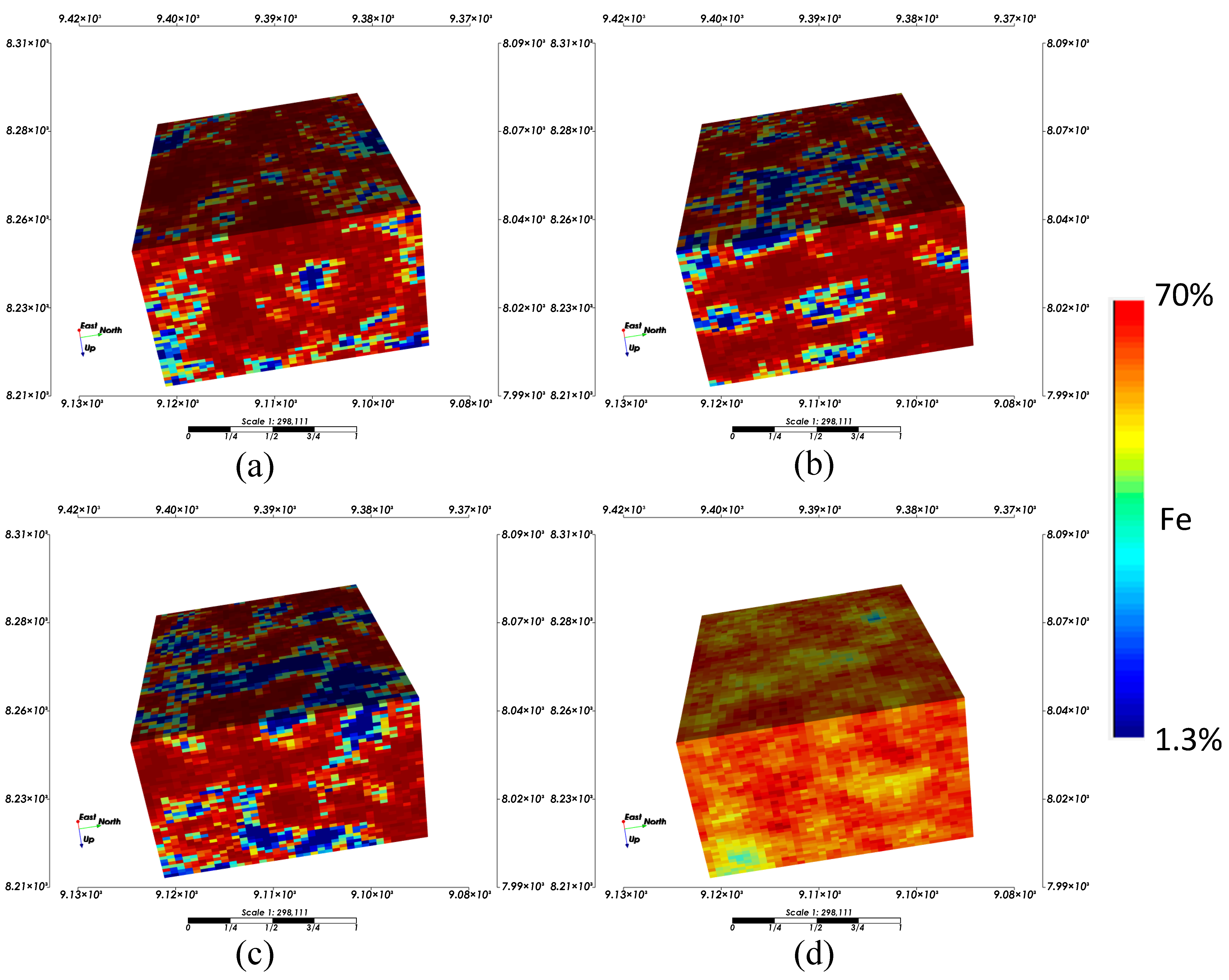
Figure 6a–c shows three SGS realizations of Fe grades. The results show that most of the area within the deposit consist of high-grade Fe with scattered low grades in a few places. These 20 simulated realizations were used in the stochastic production scheduling algorithm.
Figure 6d shows the ensemble map of the 20-simulation realization, and this model was used as the deterministic resource model for the production schedule.
5. Results and Discussion
The stochastic open-pit optimization and production schedule of the study mine uses multiple simulated orebody models generated in the previous section. The production scheduling formulation of
Section 3 was used in this study. However, this problem is the most intractable, and finding a feasible solution is NP-hard [
22,
23]. Because the production scheduling problem is NP-hard, we divided it down into a series of small sub-problems that were solved in sequence. Finally, the results of all sub-problems were integrated to obtain the main problem’s final solution. In this case study, we have applied two different techniques for solving the production scheduling problem. The first technique involves solving each sub-problem sequentially by branch and cut algorithm and improving the combined solution by using the longest path algorithm, as discussed by Lamghari and Dimitrakopoulos [
20] (hereafter referred to as Model 1). The second technique is the sequentially solving parametric maximum flow and branch and cut algorithm (hereafter referred to as Model 2). Finally, the results from both of these methods were compared. For the decision-making of the blocks to be mined, an economic block model was first created from the resource model. This was performed by considering the current production from mine, processing costs, and commodity price. For the calculation of the economic value of block i from simulation s (i.e.,
), net revenue, mining, and processing costs are used as the input. The value of block i is calculated by using the following equations [
24]:
where
The grade
is for all blocks i from simulation s are obtained from the resource model, which was generated the using sequential Gaussian simulation discussed in previous section. The geotechnical and economical parameters and the different constraint limits that are used in this case study are presented in
Table 1.
The models were solved using the CPLEX solver [
25], and the implementation was performed in a MATLAB environment. HP’s model formulation system includes an IntelI CoreTM i7-4790 processor, Windows 7, 12 GB DDR3 RAM, and a 500 GB hard drive. The model’s performance has been proved through the tolerance gap of the optimal solution and the solution time obtained by the solver.
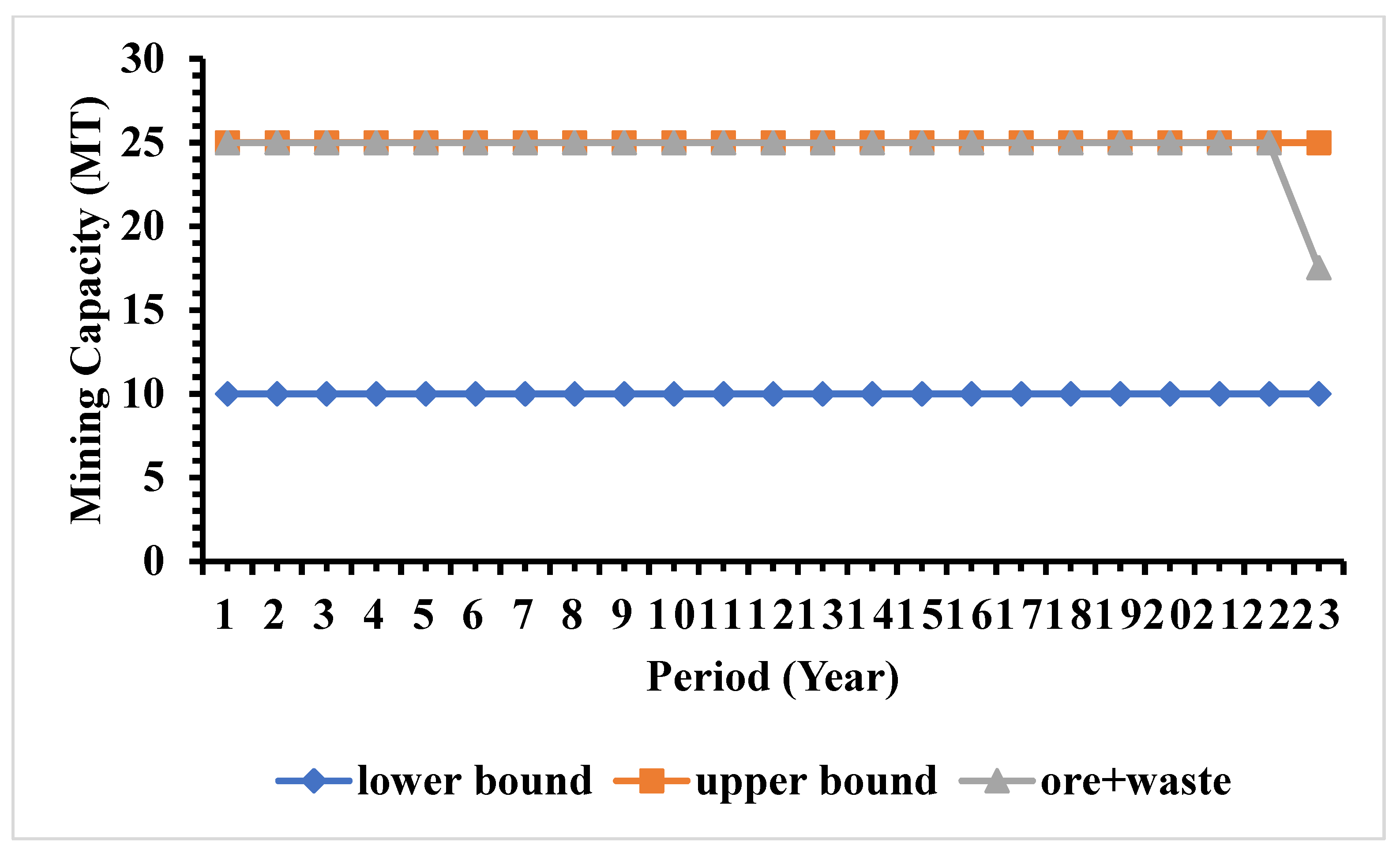
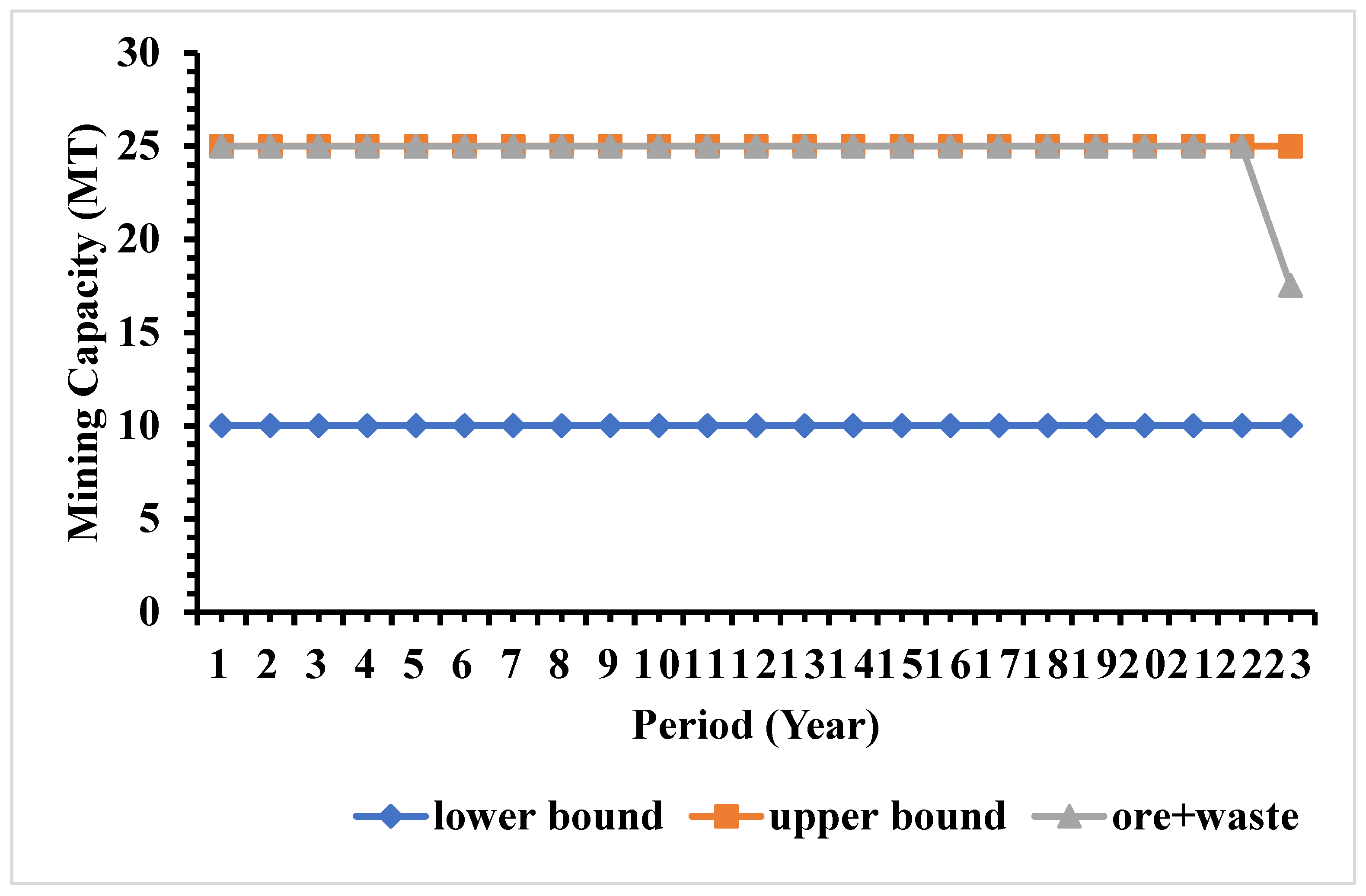
Figure 7 presents material production (i.e., mining capacity) from the deposit during production periods using Model 1.
Figure 7 shows that the production from all simulations is similar to the upper limit of the production target from the study mine for all the production periods. The results show that the optimizer tries to maximize the production to generate more cash flow. The results also show that there was no deviation from the production target. The period of production with the desired production target was 23 years.
The risk profiles of ore production capacities from different production periods were calculated using Model 1 and presented in
Figure 8. For calculating the risk profile, the stochastic production scheduling formulation using multiple block economic was first generated using Model 1. Then, from each of the simulated realizations, the total production was calculated based on the value of decision variables obtained from the production schedule for each period. The minimum, maximum, and average production were calculated from those simulated realizations for all the production periods. It was observed from
Figure 8 that the ore production constraint was not respected in the developed schedule over the production periods. During the initial periods of time, the ore production is higher than the target bounds, and, at the later periods, the ore production is lower than the target bounds. This is because the ore production constraint was relaxed with the penalty in the objective function, and, therefore, this constraint was not a hard constraint for stochastic production scheduling formulation. The penalty of the over-production at the initial periods were compensated by producing more metals from the initial period which, in turn, produces more cash inflow during the initial periods. Since the penalty due to the underproduction cannot be compensated, the optimizer tries to delay the underproduction violation, and the underproduction violation was only observed in last three periods of the mine life.
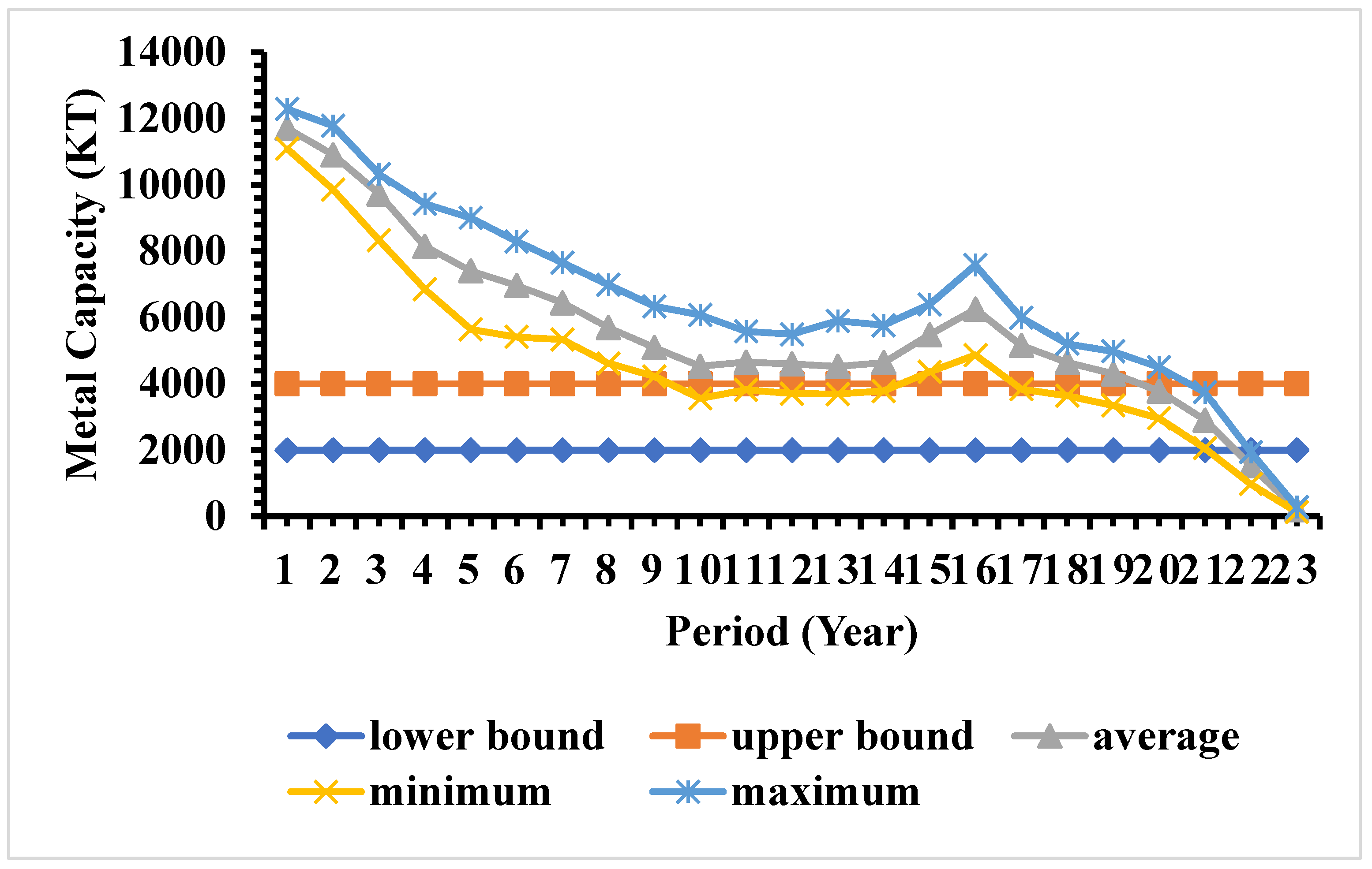
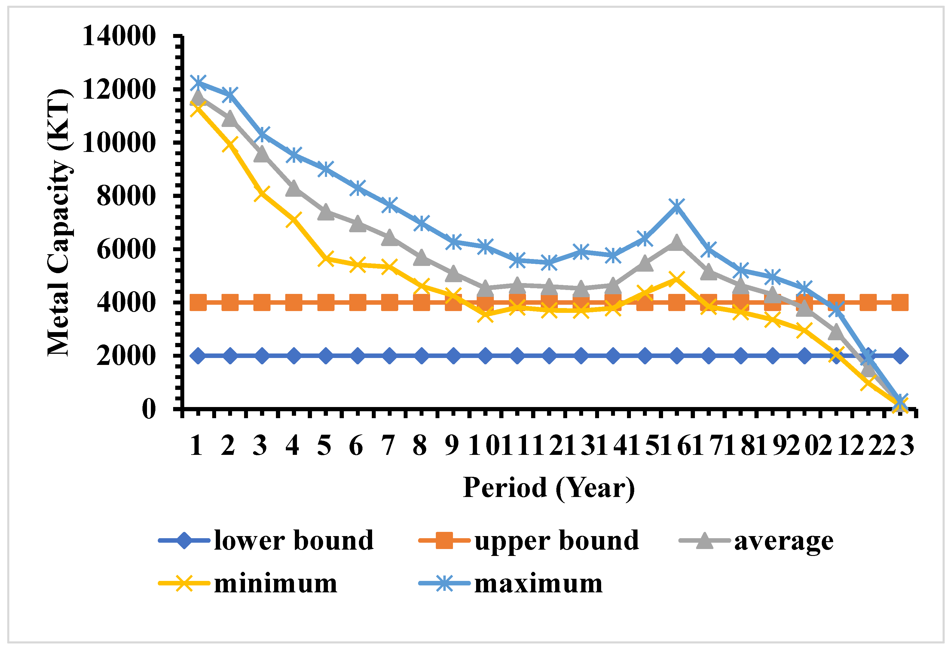
The risk profile for metal production from different production periods were calculated using Model 1 and is presented in
Figure 9. Similar to ore production, it was also observed that the metal production constraint was not respected in the generated schedule. As observed in ore production, during initial production periods, the metal production is higher than the target bound, which generates significantly high cash inflow during early mine life. The optimizer pushes the under production for the extremely late stage of the mine life. Since the goal of the production schedule is to maximize the sum of discounted cash flow, the optimizer tries to generate as much cash flow as possible during first few years, deferring the risk of not meeting the target for the later periods. The risk profile of metal production also shows that the bounds of the risk is also very tight, and it is tighter in the initial periods than later periods.
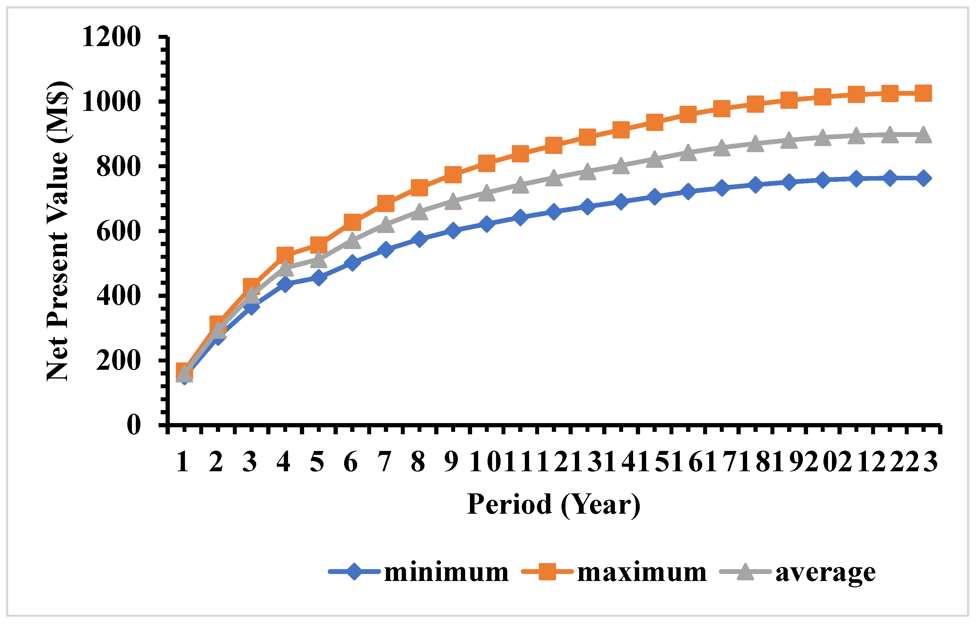
After assigning blocks to different production periods, the discounted cash flow, NPV, and their risk profiles of the deposit were calculated using Model 1 in
Figure 10. The expected NPV of the case study mine is 898 million US dollars (M
$), with a minimum and maximum NPV of 764 and 1025 million US dollars, respectively. The mining sequence along east–west section of the case study mine is presented in
Figure 11. Within the ultimate pit, the total average amount of ore is 265 Mt, and the average amount of metal is 129 Mt. The total amount of materials within the ultimate pit is 568 Mt.
The production schedule of the case study mine was then calculated using Model 2.
Figure 12 presents material production (i.e., mining capacity) from the study mine. Similar to Model 1,
Figure 12 shows that the production from all simulation is exactly same as the upper limit of the production target and that the production schedule generates steady production from the study mine. The results show that the generated schedule utilizes mining equipment at full extension to generate maximum possible materials from the study mine. Since the goal of the optimizer is to maximize the profits, the generated schedule tries to maximize the production to generate maximum cash flow. Since the production scheduling formulation does not allow for any deviation in the materials production, no deviation was observed over the mine life. Similar to Model 1, the total period of production is 23 years.
Figure 13 presents the risk profile for ore production using Model 2 over the mine life. Similar to Model 1, it was observed that the ore production constraint was not respected over the mine life. The ore production is higher than the target bound in the initial periods and then shows a decreasing trend. During the later stage of mine life, it was observed that the ore production is lower than the target bound. The trend of the ore production is more or less very similar to Model 1 due to a reason similar to the one explained before. The risk profile of Model 2 also shows similar characteristics to Model 1.
Figure 14 presents the risk profile for metal production from Model 2. Similar to ore production, the results show that the metal production constraint was violated over the mine life. Similar to Model 1, the metal production is higher than the target bound during initial production periods and lower than the target bound during extreme later stage of the mine life. The optimizer generates more cash flow during the early mine life by violating the upper limit of the metal production and pushes the under-production violation for the extremely later stage of the mine life. The risk profile of metal production also shows similar behavior to Model 1.
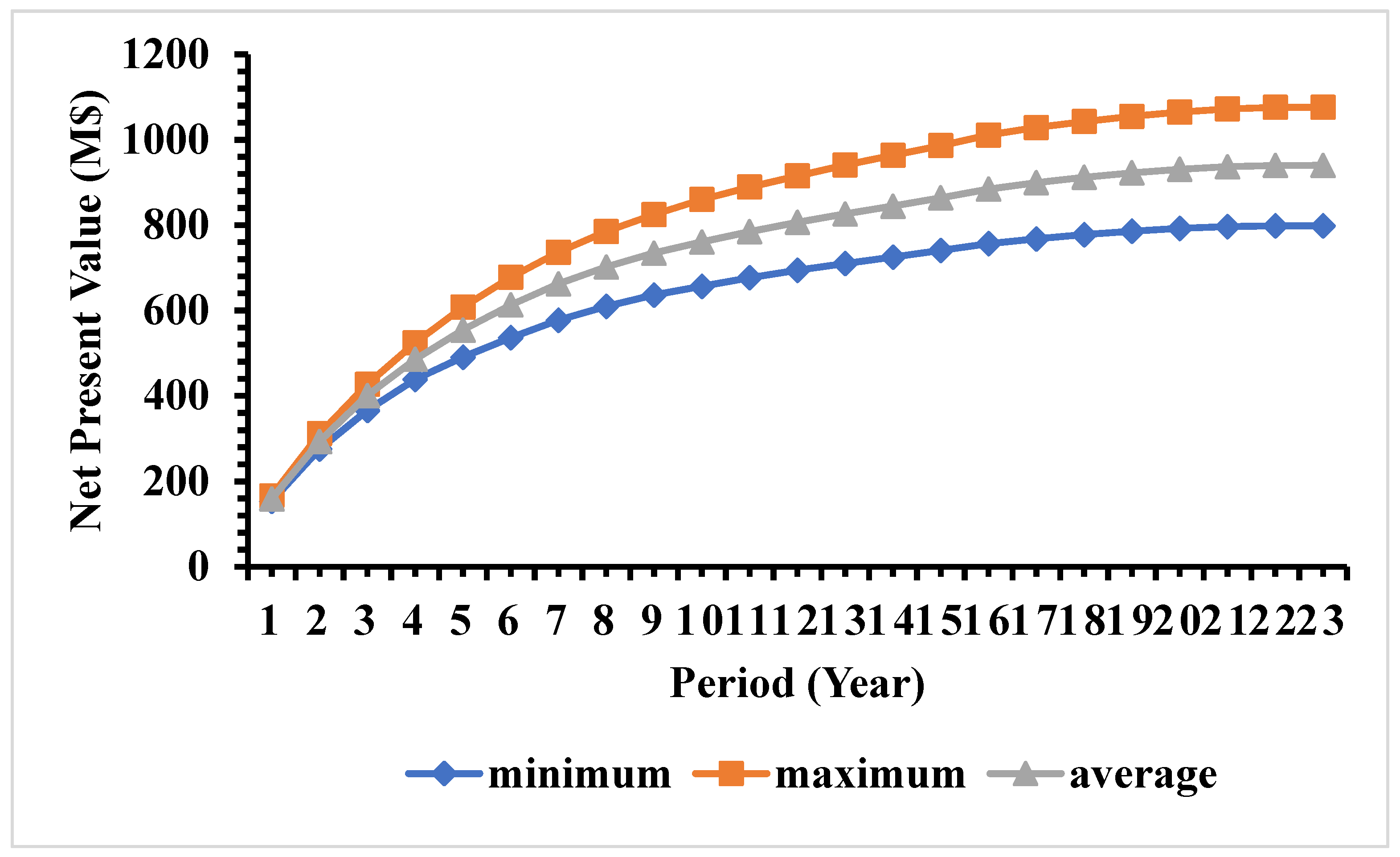
The discounted cash flow and net present value of the production schedule generated from Model 2 is presented in
Figure 15. The expected NPV of the case study mine is 940 million US dollars (M
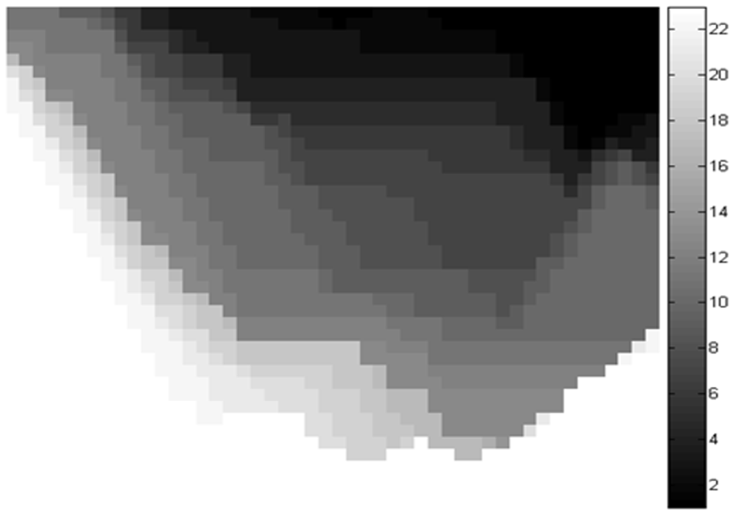
$), with a minimum and maximum NPV of 799 and 1076 million US dollars, respectively. The mining sequence along the east–west section of the case study mine is presented in
Figure 16. Within the ultimate pit, the total average amount of ore is 265 Mt, and the average amount of metal is 129 Mt. The total amount of materials within the ultimate pit is 568 Mt.
Comparison of Model 1 and Model 2
When Model 1 and Model 2 were compared, it was observed that the total mine life, material production, ore production, and metal production over the mine life are very similar to each other. The risk profiles for the ore production and metal production were similar in both models. However, it was observed that Model 2 generates slightly more revenue compared to Model 1 (4% more). This is due to a difference in the production schedule generated from these two methods. When compared the computation time, it was observed that Model 2 takes significantly less computational time as compared to Model 1. To solve the complete production scheduling problem for the study mine, Model 1 takes 2815 s, whereas Model 2 takes 1313 s.
Table 2 summaries solution time, total average metal quantity, total average discounted cash follow, and the mine life of these two models for the stochastic production scheduling of the case study mine. The detail year-wise material production, average ore and metal productions, and average NPV generated from the stochastic production schedule using both the models are presented in
Table 3.
6. Conclusions and Future Scope
This paper presents a case study from an Indian open-pit iron ore mine for stochastic production scheduling under geological uncertainty. Stochastic open-pit optimization and production scheduling is a large-scale optimization problem that greatly affects the strategic decision-making of mining industries under significant risk that comes from the uncertainty of the resource model of the deposit. To capture the uncertainty and incorporate it into the mine plan, the multiple realizations of the resource models were developed and integrated within the stochastic production scheduling framework. Two different methods were used in this case study of an iron ore mine to evaluate their performance. Model 1 is the combined branch and cut with longest path, and Model 2 is sequential parametric maximum flow and branch and cut. The results demonstrate that both the methods produce similar materials, ore, metal, and risk profiles; however, Model 2 generates slightly higher (4%) discounted cash flow as compared to Model 1 from this study mine. The results also show that the computational time of Model 2 is 46.64% less than that of Model 1. By processing the most marketable mineral output, open-pit mining’s main economic objective is to extract the least amount of material while earning the highest return on investment. The value received increases as the ore’s grade increases. A detailed operation plan that specifies how the ore body must be mined must be created in order to minimize the capital investment.
The mining industry is looking for more sophisticated tools for solving large-scale production scheduling under different uncertain environments. Traditionally, mine planners use optimization techniques that provide the highest undiscounted profits. Different mining software companies are realizing the shortcomings of traditional mine planning techniques and understanding the need to account for uncertainty in the mine plan. This case study’s results show that integrating uncertain parameters helps mine planners to see the risk in the violation of not meeting their targets, as well as the effectiveness of their cash flow analysis. The use of these optimization tools provides great opportunities for mine planners to increase returns on their investment with a high degree of confidence. The formulation and examples provided here are based on geological uncertainty; however, the same methodology can be used to account for other demand uncertainties, such as market uncertainty, commodity price, and exchange rate fluctuations, as well as mining costs, processing costs, metal recovery, and any other inputs used to determine the economic value of a mining block.
