Concentration-Temporal Multilevel Calibration of Low-Cost PM_2.5 Sensors

Abstract

Ambient aerosols have a significant impact on plant species mortality, air pollution, and climate change. It is critical to monitor the concentrations of aerosols, especially particulate matter with an aerodynamic diameter ≤ 2.5 μm (PM_2.5), which has a direct relationship with human respiratory diseases. Recently, low-cost PM_2.5 sensors have been deployed to provide a denser monitoring coverage than that of government-built monitoring supersites, which only give a macro perspective of air quality. To increase the measurement accuracy, low-cost sensors need to be calibrated. In current practice, regression techniques are used to calibrate sensors. This paper proposes a concentration-temporal multilevel calibration method to cope with the varying regression relation in different concentration and temporal domains. The performance of our method is evaluated with real field data from a supersite sensor and a low-cost sensor deployed in Puli, Taiwan. The experimental results show that our calibration method significantly outperforms linear regression in terms of R², Root Mean Square Error, and Normalized Mean Error. Moreover, our method compares favorably with a machine learning calibration method based on gradient regression tree boosting.

1. Introduction

The impact of PM_2.5 on human health has become an issue of concern globally and has motivated many governments to deploy supersite sensors for monitoring air quality. Many researchers have empirically shown the strong correlation between ambient PM_2.5 concentrations and human health [1]. As the government-built supersites need to analyze the apportionment of air pollutants, the facilitated sensors and human resources are very expensive. Since 2015, the Taiwan Environmental Protection Administration (TEPA) has collaborated with our research group, the AIRQ laboratory at National Chi Nan University (NCNU), to implement an affordable IoT of low-cost microsite PM_2.5 sensors to provide a greater and denser coverage of Puli Township, which was underserved by a single government supersite for measuring real-time air quality [2]. There are only a few studies reporting comparative performance evaluations of low-cost sensors. Manikonda et al. [3] tested four low-cost sensors under lab conditions, namely, Speck (Airviz Inc., Pittsburgh, PA, USA), Dylos 1100 Pro/Dylos 1700 (Riverside, CA, USA), AirAssure PM_2.5 IAQ Monitor (TSI Inc., Shoreview, MN, USA), and AirSense (Buffalo, NY, USA). Sayahi et al. [4] evaluated the performance of Plantower PMS 1003 in the field for more than 320 days, as well as PMS 5003 (G5). Jayaratne et al. [5] evaluated six low-cost PM_2.5 sensors, namely, Sharp GP2Y1010AU0F (Sharp-G), Shinyei PPD42NS, Plantower PMS 1003, Innocible PSM305, Nova SDS011, and Nova SDL607. Chen et al. [6] carried out a laboratory comparison between the Sharp DN7C3CA006 (Sharp-D) and Plantower PMS 3003 (3rd generation, G3) sensors, and found that G3 significantly outperformed Sharp-D in reducing the measurement offset with reference to a professional ground-truth sensor. A follow-up field verification of G3 was conducted in two places, an urban area and a petrochemical complex. The experiment results show the high stability of G3 at different locations and in various concentration ranges. Therefore, the Plantower 7th generation (G7) model PMS 7003 was deployed in our research.

Through the low-cost IoT, we superimposed real-time PM_2.5 concentrations as monitored by microsite sensors onto maps, as shown in Figure 1a, and recorded historical PM_2.5 events in order to promote public discussion. Citizens’ perceptions of air pollution can be transformed from just thinking of monolithic airsheds to being aware of local air pollution events, making them more motivated to take appropriate actions to protect themselves. For example, the PM_2.5 IoT may reveal how much residential incense and joss paper burning is contributing to local air pollution. As a result, citizens may voluntarily change their life patterns and behaviors to reduce activities that induce air pollution. The strategy of combining PM_2.5 IoT and citizen science activities is very promising in reducing environment-threatening anthropogenic activities, and this ideology has been practiced in reality around the globe, such as in the United States, Europe, and Australia, among others [7,8,9]. This solution also creates possible business models for commercial services, such as air quality data access and sensor deployment. One such example is provided by PurpleAir, Inc. (see Figure 1b).

The specifications of a standard PM_2.5 sensor equipped in a supersite station generally require precise filter holes to collect particles of the designated size, and the airflow speed should be well controlled. Then, the weight of PM_2.5 particles can be precisely measured with weighing equipment at reference temperature and humidity to calculate the concentration. On the contrary, as the microsite sensors used in the PM_2.5 IoT are low-cost, they lack the standard sampling design and procedure. Most low-cost sensors use light scattering to estimate the size and concentration of PM_2.5 particles, instead of using specified filter holes and weighing equipment. Although the measurements obtained by low-cost sensors show correlations with those obtained by supersite sensors, the relation varies to different degrees under distinct circumstances, depending on, for example, the range of PM_2.5 concentration, monitoring period in a year, location of the monitoring stations, atmospheric temperature, or relative humidity. It has been empirically proven that the correlation between supersite and low-cost sensors can be more correctly modeled if both spatial and temporal factors are taken into account in addition to just using cross-sectional data [10]. The main objective of this paper is to propose calibration equations that ensure the reliability and validity of low-cost sensors as compared with a standard supersite sensor. Moreover, our main finding is that the correlation between supersite and low-cost sensors not only shows a seasonal variability, but also manifests different magnitudes in distinct PM_2.5 concentration ranges. Clearly, it is not prudent to apply linear regression with the PM_2.5 data in the entire concentration range and across multiple years to find the relationship expression between the two types of sensors. In order to successfully run the PM_2.5 IoT with acceptable accuracy for public use, it is mandatory to calibrate the low-cost sensors with reference to standard measurements from a nearby supersite station to eliminate the measurement discrepancy [11]. The traditional numerical calibration technique adopted by TEPA is the linear regression method. Every year, TEPA announces the updated coefficient values of one linear regression expression for each supersite based on the data collected in the entire previous year. However, with our previous observations and discussions, a single linear regression expression cannot fully describe the relationships between the PM_2.5 measurement series obtained from two different types of sensors. It may potentially be beneficial to apply a separate linear regression for each typical range of PM_2.5 concentrations and monitoring time period.

The contributions of this paper are the following. (1) We propose a concentration-temporal multilevel calibration method. Both the concentration and temporal domains are divided into multiple intervals to form concentration-temporal crossing subdomains. For each subdomain, a regression is learned between historical measurements of supersite and low-cost sensors. (2) We formulate a proof that both linear regression and quadratic regression are a special case of our concentration-temporal multilevel calibration model. (3) We validate our model with various settings of concentration-temporal divisions to determine the best parameters. (4) The experimental results of the field data show that our calibration model compares favorably with classic linear regression and state-of-the-art calibration methods.

The rest of this paper is organized as follows. Section 2 describes our IoT sensors, data materials, and the proposed concentration-temporal multilevel calibration method. Section 3 presents the experimental results and comparative performance. Finally, Section 4 presents the conclusions of this work.

2. Materials and Methods

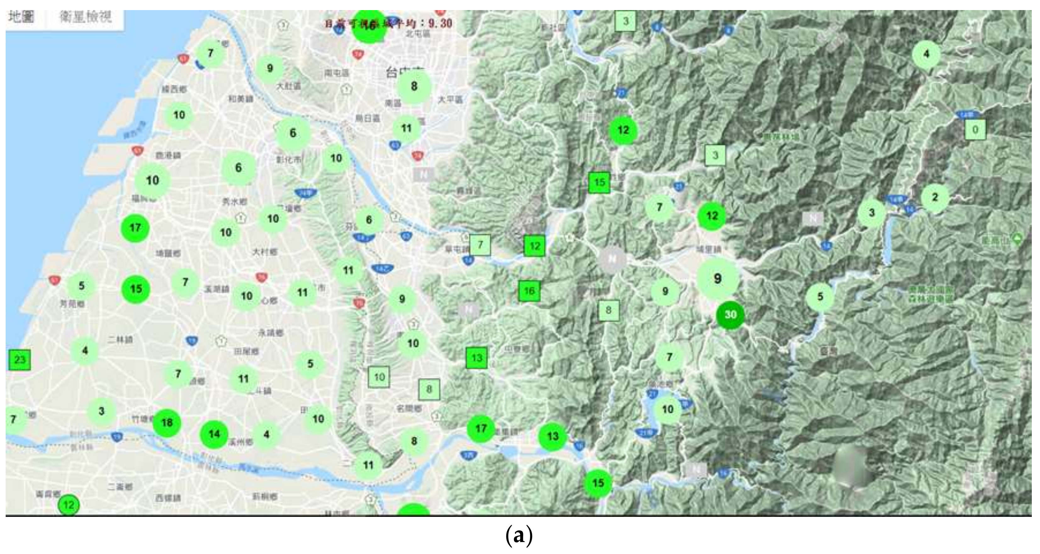
2.1. Deployment of PM_2.5 Sensor IoT

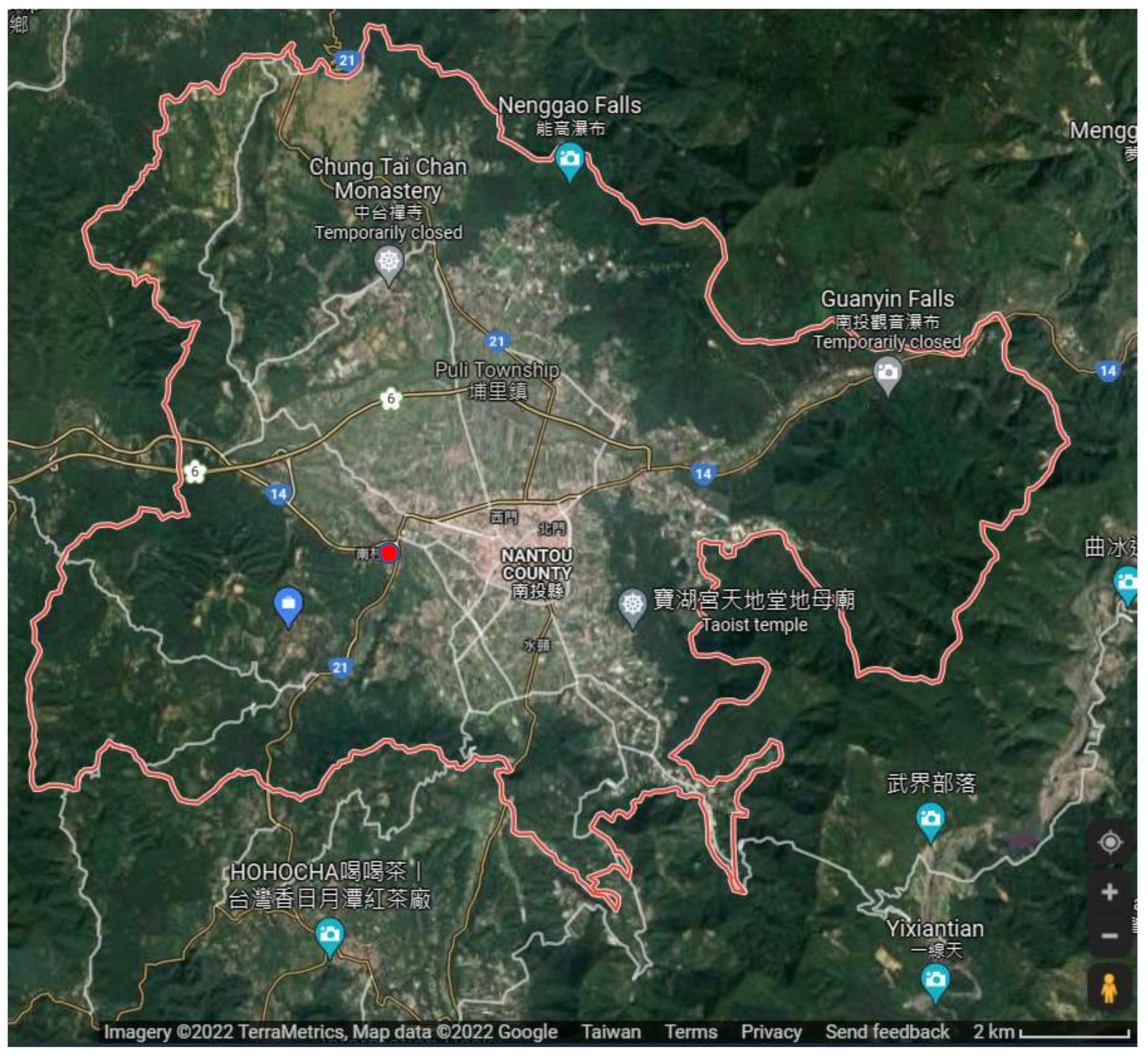
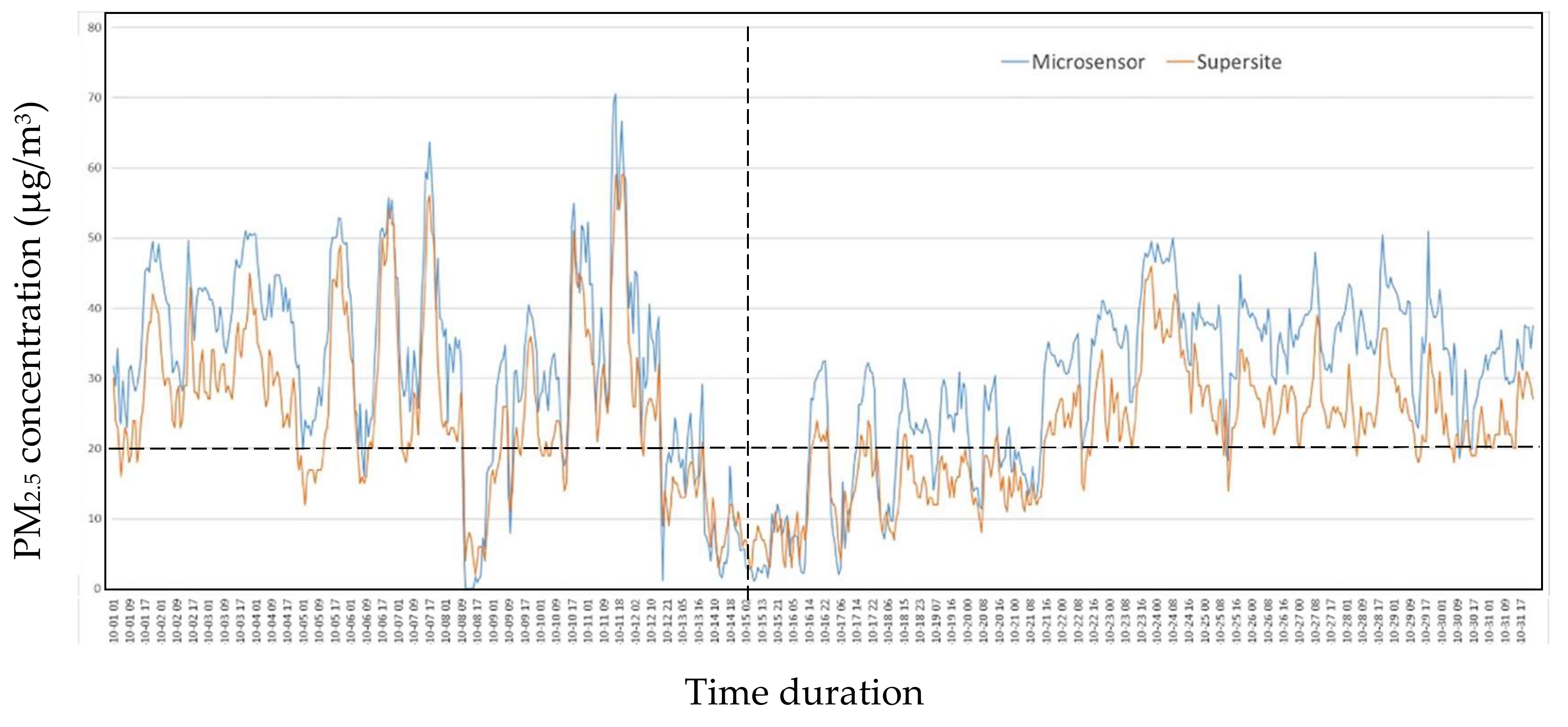
The AIRQ laboratory at NCNU has been building and maintaining an IoT of low-cost PM_2.5 sensors in Central Taiwan, including Nantou, Changhua, and Taichung, since 2015. Currently, nearly 200 monitoring microsite sensors are in operation. As previous research reported, the Plantower 7th generation (G7) model PMS 7003 shows better stability than other low-cost sensors, and therefore the AIRQ laboratory replaced the PM sensory component of the monitoring point with Plantower PMS 7003 in September 2017. The Plantower PMS 7003 has a miniature exhaust fan that sends airflow into the internal ventilation duct. Then, the interior projects laser light onto the ventilation duct and detects the scattered light with a photodiode detector. The detected amount of light is converted into a voltage, and further into a PM_2.5 value [12].

2.2. Field Study

The location of this field study is Puli Township, which is in a mountain basin of an area around 16 × 16 km² as shown in Figure 2. The height of the surrounding mountains is between 1000 and 3500 m. TEPA has deployed only one monitoring supersite station (marked by a red dot in Figure 2) in the basin because Puli Township is in a rural area and the main occupation is agriculture. However, there are occasional crop burning activities in farms, and lots of tourists visit Puli at weekends. The only TEPA supersite definitely cannot provide a full coverage for air quality monitoring of Puli, especially for detecting local emerging air pollution events. This motivates our field study for establishing a PM_2.5 IoT of low-cost G7 sensors.

To publicize the use of our PM_2.5 IoT to Puli citizens, the measurement of G7 sensors should be calibrated before the deployment. We placed a G7 sensor in a spacious corridor of an elementary school, which is next to the TEPA supersite station, with no buildings or obstacles in between the two sites. Conspicuously, the two monitoring sites are close enough and with similar ventilation and background air conditions. This field arrangement provides a feasible and fair comparison between the TEPA supersite and the low-cost sensor for the IoT deployment.

The time span of the field study is from 1 January 2018 to 31 December 2019. We recorded hourly PM_2.5 measurements from both the TEPA supersite and the microsite G7 sensor. Data from the whole of the year 2018 are used for training the comparative models, and data from the year 2019 are used for testing.

As previously mentioned, we found that the correlation between the supersite and low-cost sensors not only shows a seasonal variability, but also manifests different magnitudes in distinct PM_2.5 concentration ranges. For example, Figure 3 shows a comparison between the hourly measurements of the TEPA supersite in Puli Township (orange curve) and a nearby low-cost sensor (blue curve). It can be seen that the two measurement time series have similar trends; however, they have different correlation degrees in various time and concentration regions. The value difference between the two measurement time series is relatively small when the measurements of the TEPA supersite are below 20 µg/m³, and the difference proliferates when the measurements are above 20 µg/m³. Analogously, the difference between the two measurement time series is relatively smaller in the first half of October than in the second half. Clearly, it is not prudent to apply linear regression with the PM_2.5 data in the entire concentration range and across multiple years to find the relationship expression between the supersite and low-cost sensors. We propose improving the accuracy of calibration learned in different segments of concentration range and time duration.

2.3. Concentration-Temporal Multilevel Calibration Model

The traditional calibration method adopted by TEPA is the linear regression (LR) model, which intends to find a linear function relating the measurement of a calibrating sensor to that of a reference sensor based on the data of the entire past year. Let the measurement of the calibrating sensor at hour i be x_i, and the measurement of the reference sensor at hour i be y_i. Linear regression (Equation (1)) minimizes the difference between y_i and the calibrated value of x_i over all measurements.

$$Minimize \sqrt{\frac{{{\displaystyle \sum }}_{i=1}^n{\left(y_i-\widehat{x_i}\right)}^2}{n}},{ }_{}\widehat{x_i}=w_1{x}_i+w_0$$

(1)

where w₁ is the regression coefficient, w₀ is the residue, $\widehat{x_i}$ is the calibrated value of x_i, and n is the number of measuring hours.

Some References [13,14] have found that quadratic regression (QR) may be more useful than LR for estimating the PM_2.5 concentration in particular cities. QR calibrates the measurement by Equation (2).

$$\widehat{x_i}=w_2{x}_i^2+w_1{x}_i+w_0$$

(2)

where w₁ and w₂ are the regression coefficients and w₀ is the residue.

In this paper, we propose a concentration-temporal multilevel linear regression (CTMLR) method for improving the sensor calibration accuracy. As previously noted, we found that the correlation between the supersite and low-cost sensors shows variations in both PM_2.5 concentration and temporal domains. The performance of sensor calibration is likely to improve if the regression can be conducted separately in the concentration-temporal crossing intervals. Let the concentration domain be divided into J ranges, C_j, j = 1, 2, …, J, and the temporal domain into K ranges, T_k, k = 1, 2, …, K. The division can be made uniformly or non-uniformly considering the distributions of historical measurements. For convenience of presentation, we assume the corresponding concentration and temporal intervals of x_i are C_j and T_k, respectively. The CTMLR method employs the following multilevel linear regression (Equation (3)) to calibrate the measurement.

$$\widehat{x_i}=w_1\left(C_j,T_k\right)x_i+w_0\left(C_j,T_k\right), \forall j=1,2,\dots ,J; k=1,2,\dots ,K$$

(3)

where w₁(C_j, T_k) is the regression coefficient and w₀(C_j, T_k) is the residue. The difference between CTMLR and LR is that both w₁(C_j, T_k) and w₀(C_j, T_k) used in CTMLR are a concentration-temporal function in terms of C_j and T_k. Meanwhile in LR, w₁ and w₀ are just scalar values, which are independent of the observed concentration (x_i) and time (hour i). Consequently, CTMLR employs a form for learning the weight function in the concentration-temporal domain. In the following, we show that both LR and QR are a special case of CTMLR, so the latter can learn a more sophisticated relationship between the measurements of supersite and microsite sensors.

Theorem 1.

Both LR and QR are a special case of CTMLR.

Proof. 

For LR, assume the learned regression form is $\widehat{x_i}=w_1{x}_i+w_0$.We can let w₁(C_j, T_k) and w₀(C_j, T_k) be fixed constant values for all combinations of concentration and temporal domains, i.e.,

$$w_1\left(C_j,T_k\right)=w_1; w_0\left(C_j,T_k\right)=w_0, \forall j=1,2,\dots ,J; k=1,2,\dots ,K$$

(4)

So, CTMLR reduces to LR.

For QR, let the learned regression form be $\widehat{x_i}=w_2{x}_i^2+w_1{x}_i+w_0$. We consider CTMLR learns the following weight functions.

$$w_1\left(C_j,T_k\right)=w_2{C}_j+w_1; w_0\left(C_j,T_k\right)=w_0, \forall j=1,2,\dots ,J; k=1,2,\dots ,K$$

(5)

Then, Equation (3) derives to $\widehat{x_i}=w_2{C}_j{x}_i+w_1{x}_i+w_0$. If we conduct the finest range division in the concentration domain, viz., C_j = x_i, CTMLR derives to the following regression form.

$$\widehat{x_i}=w_2{x}_i{x}_i+w_1{x}_i+w_0=w_2{x}_i^2+w_1{x}_i+w_0,$$

(6)

which is exactly the QR regression form.

To conclude the proof, LR is a special case of CTMLR with a single range of the entire concentration-temporal domain, and QR can be learned through CTMLR if we conduct the finest division in the concentration domain and no division in the temporal domain. □

To make the CTMLR method more computationally efficient, the regression can be only conducted in those concentration-temporal crossing domains that contain a significant number of historical measurements from the reference and calibrating sensors. The optimal weight functions of CTMLR can be learned by applying any feasible optimization approach. In this study, we employ particle swarm optimization (PSO) [15] to learn the weight functions in every concentration-temporal crossing domain because PSO is computationally fast and converges to quality local optima in practice.

2.4. Performance Indicators

In the following, the broadly used performance indicators for evaluating calibration methods are introduced.

Coefficient of Determination (R²)

$$R^2=1-\frac{{{\displaystyle \sum }}_{i=1}^n{\left(y_i-\widehat{x_i}\right)}^2}{{{\displaystyle \sum }}_{i=1}^n{\left(y_i-\overline{y}\right)}^2}$$

(7)

where $\overline{y}$ is the mean observed value of all reference measurements,

$$\overline{y}=\frac{{{\displaystyle \sum }}_{i=1}^n{y}_i}{n}$$

(8)

Root Mean Square Error (RMSE)

$$RMSE=\sqrt{\frac{{{\displaystyle \sum }}_{i=1}^n{\left(y_i-\widehat{x_i}\right)}^2}{n}}$$

(9)

Normalized Mean Error (NME)

$$NME=\frac{{{\displaystyle \sum }}_{i=1}^n\left|y_i-\widehat{x_i}\right|}{{{\displaystyle \sum }}_{i=1}^n\left(y_i\right)}$$

(10)

Except for R² which is the higher the better, the other indicators are to be minimized in the calibration process.

3. Results

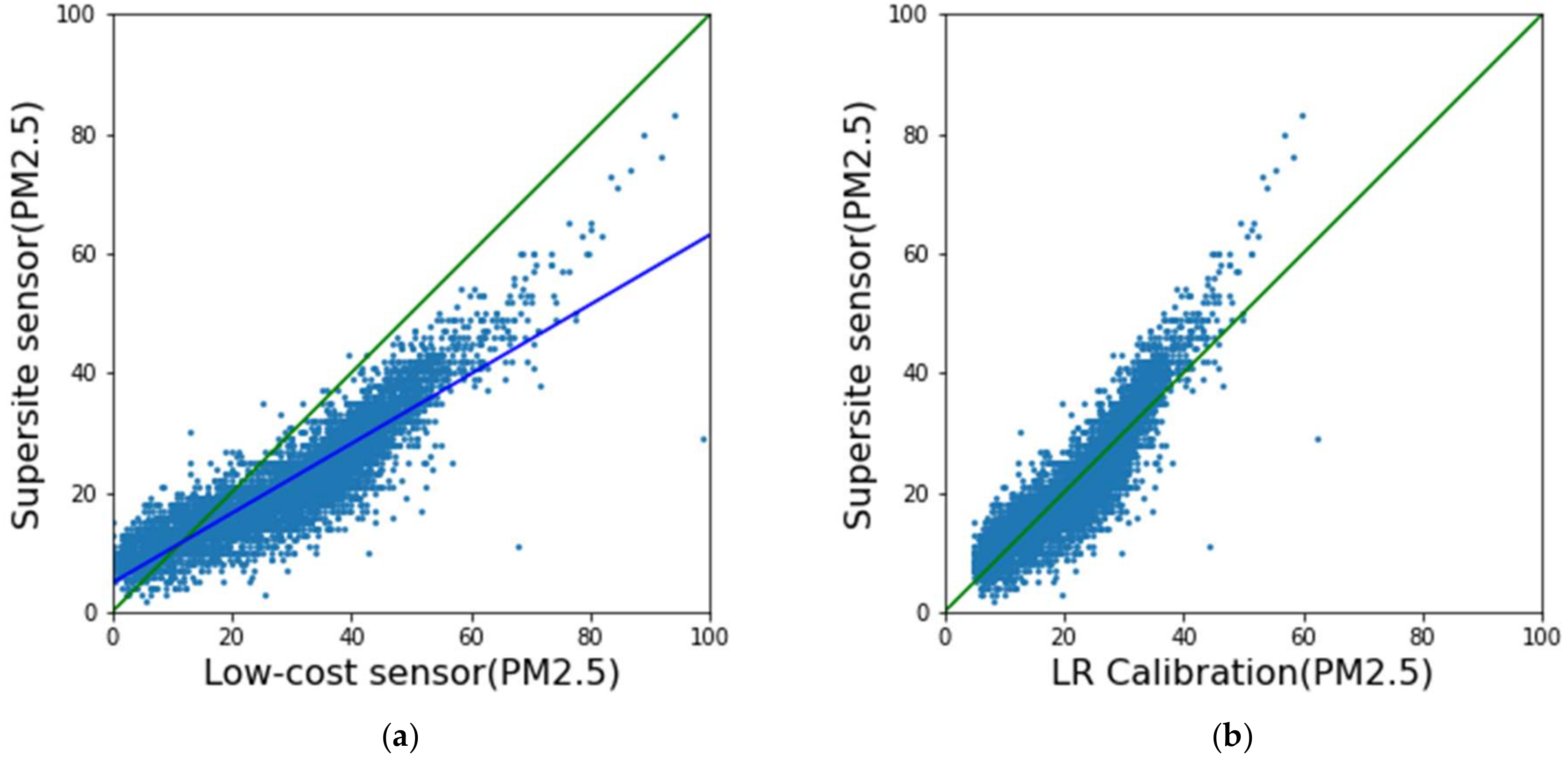
3.1. Validation of CTMLR Calibration

We validate the CTMLR calibration method with our low-cost G7 PM_2.5 sensor deployed near to the TEPA Puli supersite. The time span of the collected PM_2.5 hourly measurements is from 1 January 2018 to 31 December 2019. The data from the year 2018 are used for training, and the data from the year 2019 are used for testing. We first calibrate the low-cost sensor with reference to the Puli supersite with the classic LR method. The result will be used as baseline performance for evaluating the CTMLR calibration method. We then analyze the influence of using various lengths of division interval for slicing the concentration and temporal domains in the performance of CTMLR calibration. To this end, we experiment with setting the length of the division interval in the concentration domain to 5, 10, 15, 20, and 25, respectively. The temporal domain is divided by month, season, or year. For each parameter combination of concentration-temporal division, the resulting CTMLR version is trained with data from the year 2018. The testing performance on data from the year 2019 achieved by various versions of CTMLR is shown in

Table 1. Testing performance evaluation of the CTMLR and LR calibration methods.

Indicators	Temporal	Concentration (µg/m3)
		5	10	15	20	25	LR
R2	month	79%	79%	79%	79%	79%	78%
	season	80%	80%	80%	80%	80%	78%
	year	82.81%	82.85%	82.87%	82.7%	82.6%	80%
RMSE	month	4.99	4.9	4.9	4.9	4.9	5.0
	season	4.8	4.8	4.8	4.8	4.8	5.0
	year	4.51	4.503	4.502	4.52	4.53	4.7
NME	month	0.22	0.22	0.21	0.22	0.22	0.22
	season	0.21	0.21	0.21	0.21	0.21	0.22
	year	0.1939	0.1938	0.1937	0.194	0.196	0.20

, which also includes the baseline LR performance. It can be seen that for all performance indicators, CTMLR outperforms LR for every parameter combination of concentration-temporal division. The result validates that CTMLR is more capable than LR of rendering the relationship between the low-cost sensor and the reference supersite sensor.

We further analyze the best division parameters for creating the multilevel concentration-temporal crossings for the Puli dataset. From the performance evaluation shown in Table 1, we observe that the best calibration result (shown in bold) for all performance indicators is always obtained by dividing the concentration domain with an interval of 15 µg/m³ and using the entire year as the temporal interval. The implication is that the correlation between the two types of sensors varies more significantly in the concentration domain than the temporal domain. The reason for this is that the major PM_2.5 concentration range in a month or a season is relatively typical, so many concentration-temporal crossings contain too few data to learn representative regression on a monthly or a seasonal basis. For the best division parameter in the concentration domain, we further test with finer divisions between 15 and 20 µg/m³. As shown in

Table 2. Finer testing performance evaluation of the CTMLR calibration method.

Indicators	Temporal	Concentration (µg/m3)
		15	16	17	18	19	20
R2	month	79%	79%	79%	80%	79%	79%
	season	80%	80%	80%	80%	80%	80%
	year	82.873%	82.868%	82.82%	82.80%	82.80%	82.76%
RMSE	month	4.9	5.0	5.0	4.9	4.9	4.9
	season	4.8	4.8	4.8	4.8	4.8	4.8
	year	4.502	4.501	4.51	4.51	4.52	4.52
NME	month	0.21	0.22	0.22	0.22	0.22	0.22
	season	0.21	0.21	0.21	0.21	0.21	0.21
	year	0.1937	0.1936	0.194	0.195	0.195	0.195

, the best calibration performance in terms of R² is obtained with an interval division of 15 µg/m³, while the best performance in terms of RMSE and NME is obtained when the concentration interval division is set to 16 µg/m³. The two interval lengths are very close, showing the stability of our CTMLR calibration method against different performance indicators. Again, the best performance in all indicators is produced with the temporal interval of an entire year to collect a sufficient number of samples.

With the best parameters for training the CTMLR calibration method, we visualize the difference in training performance between CTMLR and LR by comparing their scatter plots. Figure 4a shows the scatter plot of the supersite sensor and low-cost sensor before calibration. The blue line depicts the principal axis of the plots, and the green line indicates the ideal line y = x. It can be seen that the original plots are tilted away from the ideal line. With the LR calibration result as shown in Figure 4b, the plots are drawn closer to the ideal line. However, the upper-right region of the plots (for supersite measurements between 40 and 90 µg/m³) crosses the ideal line to the other side. As a comparison, we apply CTMLR calibration to the training data. The calibrated plots perfectly align with the ideal line as shown in Figure 4c. The is because CTMLR applies multilevel linear regression in the concentration domain and is able to adjust the weights in the upper-right region of the plots. Clearly, the learning capability of CTMLR significantly outperforms that of LR.

For the testing data, the original plots of the supersite sensor and low-cost sensor before calibration are displayed in Figure 5a. Again, the blue line is tilted away from the ideal green line. By applying the LR calibration method to the testing data, as shown in Figure 4b, the plots align with the ideal line. However, the central region of the plots is a little lower than the ideal line. On the other hand, the CTMLR calibration method generalizes better to the testing data than the LR method. The calibrated plots uniformly are distributed over the ideal line as shown in Figure 5c. The calibration effectiveness of the CTMLR method is due to the multilevel regression in the concentration-temporal crossing domain. The CTMLR method is a generalized model of LR and QR as we have previously proven. The multilevel regression mechanism enables the flexibility of the CTMLR method in fitting to various distribution forms manifested in different subdomains.

3.2. Comparison with Other Calibration Methods

In this section, the proposed CTMLR approach is compared with state-of-the-art calibration methods. XGBoost is a gradient-based boosting algorithm [16] for learning regression trees, and it has won several machine learning competitions such as Kaggle challenges and the KDD Cup. Ensemble XGBoost [6] is a novel calibration method, which constructs an ensemble for learning spatiotemporal parameters in order to build XGBoost regression trees. Three versions of XGBoost regression trees were constructed in [6] by using the Sobol [17], Nelder and Meads (N&M) [18], and PSO [15] methods, respectively. We applied the three versions of XGBoost regression trees to calibrate the low-cost sensor with the TEPA Puli dataset. The testing calibration performance of the three XGBoost ensembles is shown in

Table 3. Testing performance evaluation of the three XGBoost ensembles.

Indicators	XGBoost Ensembles
	Sobol	N&M	PSO
R2	80%	78%	80%
RMSE	5.7	5.8	5.7
NME	0.173	0.18	0.175

. It can be seen that Sobol-learned XGBoost is the best version overall, though its R² value is slightly worse than that obtained by PSO-learned XGBoost. We then compare Sobol-learned XGBoost with our CTMLR approach (see Table 1 and Table 2). Clearly, CTMLR outperforms Sobol-learned XGBoost in terms of R² and RMSE measurements. However, Sobol-learned XGBoost is able to achieve a better NME value than CTMLR. The implication is that CTMLR tends to calibrate the sensors by normally distributing the main error residues to all samples, such that a lower R² or RMSE value can be obtained (see the quadratic expression in Equations (7) and (9)). On the other hand, Sobol-learned XGBoost focuses on minimizing error residues in most samples while allowing the existence of larger residues in the remaining samples (see the NME L₁-norm expression in Equation (10)). In summary, CTMLR and Sobol-learned XGBoost are both effective in calibration, and they may fit better in different measurement scenarios.

4. Conclusions

This paper proposes an affordable low-cost sensor IoT to provide a complementary microlevel air quality perspective for individual needs. Measurements from low-cost sensors have a varying relationship with those from supersite sensors. The variables influencing this relationship, at the least, include meteorological, spatial, temporal, and concentration factors. We propose a concentration-temporal multilevel linear regression (CTMLR) method for improving the calibration accuracy of low-cost sensors. We also show that the classic calibration methods, namely, linear regression (LR) and quadratic regression (QR), are special cases of the CTMLR method. In other words, the CTMLR method is more general than LR and QR, and it is capable of rendering the complex relationship between supersite sensors and low-cost sensors. The experimental results with the field data show that the CTMLR method outperforms LR with reference to all popular calibration measures. When compared with Ensemble XGBoost, which is one of the state-of-the-art calibration methods, CTMLR surpasses two versions of Ensemble XGBoost and is comparable to another version that is trained by the Sobol optimizer.

Our future research scope includes the following directions. In the present study, the CTMLR method is facilitated by fixed-length intervals in both the concentration and temporal domains. It would be worthwhile to study whether the calibration performance of the CTMLR method improves when varying-length intervals are considered in the training. Another direction for our future research is to include other calibration variables in the CTMLR method. Some useful variables suggested in the literature include meteorological, spatial, and land use factors. Such a hybrid model has the potential to adapt to different field scenarios that are not sufficiently described by a single type of calibration variable.

References

1. Song, C.; He, J.; Wu, L.; Jin, T.; Chen, X.; Li, R.; Ren, P.; Zhang, L.; Mao, H. Health burden attributable to ambient PM2.5 in China. Environ. Pollut. 2017, 223, 575–586. [Google Scholar] [CrossRef] [PubMed]
2. Day, R.F. Developing the Local PM2.5 Monitoring System and the Volunteer Program for Air Protection; Technical Report EPA024 105025; Environmental Protection Administration, Executive Yuan, R.O.C.: Taipei, Taiwan, 2017. [Google Scholar]
3. Manikonda, A.; Zíková, N.; Hopke, P.K.; Ferro, A.R. Laboratory assessment of low-cost PM monitors. J. Aerosol Sci. 2016, 102, 29–40. [Google Scholar] [CrossRef]
4. Sayahi, T.; Butterfield, A.; Kelly, K. Long-term field evaluation of the Plantower PMS low-cost particulate matter sensors. Environ. Pollut. 2019, 245, 932–940. [Google Scholar] [CrossRef] [PubMed]
5. Jayaratne, R.; Liu, X.; Ahn, K.-H.; Asumadu-Sakyi, A.; Fisher, G.; Gao, J.; Mabon, A.; Mazaheri, M.; Mullins, B.; Nyaku, M. Low-cost PM2. 5 sensors: An assessment of their suitability for various applications. Aerosol Air Qual. Res. 2020, 20, 520–532. [Google Scholar]
6. Chen, L.J.; Ho, Y.H.; Lee, H.C.; Wu, H.C.; Liu, H.M.; Hsieh, H.H.; Huang, Y.T.; Lung, S.C.C. An open framework for participatory PM2.5 monitoring in smart cities. IEEE Access 2017, 5, 14441–14454. [Google Scholar] [CrossRef]
7. Jiao, W.; Hagler, G.; Williams, R.; Sharpe, R.; Brown, R.; Garver, D.; Judge, R.; Caudill, M.; Rickard, J.; Davis, M. Community Air Sensor Network (CAIRSENSE) project: Evaluation of low-cost sensor performance in a suburban environment in the southeastern United States. Atmos. Meas. Tech. 2016, 9, 5281–5292. [Google Scholar] [CrossRef] [PubMed]
8. Morawska, L.; Thai, P.K.; Liu, X.; Asumadu-Sakyi, A.; Ayoko, G.; Bartonova, A.; Bedini, A.; Chai, F.; Christensen, B.; Dunbabin, M. Applications of low-cost sensing technologies for air quality monitoring and exposure assessment: How far have they gone? Environ. Int. 2018, 116, 286–299. [Google Scholar] [CrossRef] [PubMed]
9. English, P.; Richardson, M.; Garzón-Galvis, C. From crowdsourcing to extreme citizen science: Participatory research for environmental health. Annu. Rev. Public Health 2018, 39, 335–350. [Google Scholar] [CrossRef] [PubMed]
10. Yin, P.Y.; Tsai, C.C.; Day, R.F.; Tung, C.Y.; Bhanu, B. Ensemble learning of model hyperparameters and spatiotemporal data for calibration of low-cost PM2.5 sensors. Math. Biosci. Eng. 2019, 16, 6858–6873. [Google Scholar] [CrossRef] [PubMed]
11. Castell, N.; Dauge, F.R.; Schneider, P.; Vogt, M.; Lerner, U.; Fishbain, B.; Broday, D.; Bartonova, A. Can commercial low-cost sensor platforms contribute to air quality monitoring and exposure estimates? Environ. Int. 2017, 99, 293–302. [Google Scholar] [CrossRef] [PubMed]
12. Kelly, K.; Whitaker, J.; Petty, A.; Widmer, C.; Dybwad, A.; Sleeth, D.; Martin, R.; Butterfield, A. Ambient and laboratory evaluation of a low-cost particulate matter sensor. Environ. Pollut. 2017, 221, 491–500. [Google Scholar] [CrossRef] [PubMed]
13. Yin, Q.; Wang, J.; Hu, M.; Wong, H. Estimation of daily PM2.5 concentration and its relationship with meteorological conditions in Beijing. J. Environ. Sci. 2016, 48, 161–168. [Google Scholar] [CrossRef] [PubMed]
14. Baker, K.R.; Foley, K.M. A nonlinear regression model estimating single source concentrations of primary and secondarily formed PM2.5. Atmos. Environ. 2011, 45, 3758–3767. [Google Scholar] [CrossRef]
15. Kennedy, J.; Eberhart, R.C. Particle swarm optimization. In Proceedings of the IEEE International Conference on Neural Networks IV, Perth, WA, Australia, 27 November–1 December 1995; pp. 1942–1948. [Google Scholar]
16. Chen, T.; Guestrin, C. XGBoost: A scalable tree boosting system. In Proceedings of the 22nd ACM SIGKDD International Conference on Knowledge Discovery and Data Mining (KDD2016), San Francisco, CA, USA, 13–17 August 2016. [Google Scholar]
17. Joe, S.; Kuo, F.Y. Remark on algorithm 659: Implementing Sobol’s quasirandom sequence generator. ACM Trans. Math. Softw. (TOMS) 2003, 1, 49–57. [Google Scholar] [CrossRef]
18. Lagarias, J.C.; Reeds, J.A.; Wright, M.H. Convergence properties of the Nelder-Mead simplex method in low dimensions. SIAM J. Optim. 1998, 9, 112–147. [Google Scholar] [CrossRef]
Figure 1. Low-cost PM2.5 IoT solutions: (a) AIRQ lab at NCNU (https://www.airq.org.tw/ (accessed on 1 July 2022)) (translation of Chinese symbols: Map; Satellite Monitor; Current average of visible area) and (b) PurpleAir, Inc. (https://www.purpleair.com/ (accessed on 1 July 2022)).
Sustainability 14 10015 g001aSustainability 14 10015 g001b
Figure 2. Puli Township is in a mountain basin, and there is only one government-built PM2.5 monitoring supersite (marked by a red dot) (translation of Chinese symbols: Wujie Tribe).
Sustainability 14 10015 g002
Figure 3. In various segments of PM2.5 concentration range and time duration, the measurements of low-cost sensors show different degrees of deviation from the standard measurements.
Sustainability 14 10015 g003
Figure 4. Scatter plots for the training data: (a) before calibration, (b) after LR calibration, and (c) after CTMLR calibration.
Sustainability 14 10015 g004aSustainability 14 10015 g004b
Figure 5. Scatter plots for the testing data: (a) before calibration, (b) after LR calibration, and (c) after CTMLR calibration.
Sustainability 14 10015 g005aSustainability 14 10015 g005b