Reliability Assessment Method for Simply Supported Bridge Based on Structural Health Monitoring of Frequency with Temperature and Humidity Effect Eliminated

Abstract

Structural health monitoring (SHM) has been widely used for the performance assessment of bridges, especially the methods based on dynamic characteristics. Meanwhile, bridge modal frequency is influenced significantly by environmental factors, such as temperature and humidity. Combined with SHM, a reliability assessment of bridges with the temperature and humidity effects eliminated is proposed. Firstly, the bridge deflection verification coefficient is adopted as the evaluation indicator for bridge condition, which is the ratio of deflection-measured value to deflection-calculated value. It is obtained from the relationship between verification coefficient and modal frequency through theoretical derivation. Secondly, a back propagation (BP) neural network is improved by using an artificial bee colony algorithm and employed as a surrogate model to eliminate the effect of temperature and humidity on frequency. Thirdly, a dynamic Bayesian network is applied to establish the reliability analysis model combined with the monitoring results, so that the probability distribution of bridge parameters is updated to improve the accuracy of the reliability analysis. Finally, a simply supported bridge is used as the case study, based on the proposed method in this work. The results indicate that the proposed method can eliminate the temperature and humidity effect on frequency precisely and effectively. With the effect of temperature and humidity on frequency eliminated, the bridge condition assessment can be evaluated accurately through the reliability analysis based on SHM and the dynamic Bayesian network.

1. Introduction

As a key component of the transportation network, bridges make essential contribution to social and economic development. However, with service time increasing, bridges become deteriorated under the action of vehicle load and adverse environmental factors [1]. According to the report from the Ministry of Transport of China, 76,483 highway bridges in China had structurally deficient ratings [2]. Moreover, in California, USA, structurally deficient bridges increased from 6.2% to 7% of total bridges [3]. Therefore, structural health monitoring (SHM) has been a hotspot in the research of bridge condition assessment in recent years. The accurate evaluation of a bridge’s condition for the reliability and sustainability of bridge service performance, which can be carried out by SHM, is of great significance [4,5].

Having benefitted from the development of sensor and communication technology, the SHM of bridges has developed rapidly, and is formed based on acoustic characteristics [6], graphic information [7], and static response [8] as monitoring indexes. Meanwhile, the vehicle load action and external environmental factors can be obtained accurately [9,10]. The SHM based on structural modal parameters becomes the main monitoring technology due to the advantages of mature technology, higher accuracy, and continuous monitoring [11]. There are two categories of the vibration-based SHM, namely a direct type and an indirect type. The direct method is based on the accelerometer arranged on bridges to extract the dynamic parameter [12], and the indirect method is carried out through vehicle-assisted techniques [13]. The damage identification and performance evaluation of bridges are studied using SHM of modal frequency and mode shape. Lee et al. used time domain decomposition techniques from vibration-based SHM to extract mode shape [14]. Liu et al. established a baseline finite element model including material properties, spring bearing elements, and the replacement of Mindlin plate elements, which is used for real-time damage identification and SHM [15]. Li et al. proposed a new method to extract the time-dependent characteristics of the bridge with vehicles moving, and it was validated through laboratory and field tests that the proposed method evaluated the bridge condition accurately [16]. However, the above SHM technologies and methods based on dynamic performance are only effective for the identification of local damage and dynamic characteristic assessment, and they are prone to the interference of monitoring noise and external environment factors.

Among them, the influence of ambient temperature on the modal frequency is particularly significant, which affects the material and structural properties of bridges directly. Even worse, it masks the changes caused by bridge damage, and leads to the distortion of bridge performance analysis [17]. Therefore, it is very important to eliminate the effect of temperature on bridge condition assessment. Based on research about the long-term monitoring data of bridge frequency and ambient temperature, it was demonstrated that temperature had a negative correlation with frequency [18]. The influence of temperature on geometrical dimensions, boundary conditions, and the elastic modulus of a bridge was analyzed through experimental analysis, numerical simulation, and a neural network. The numerical relationship between structural elastic modulus and ambient temperature was clarified, and the effect mechanism of temperature on bridge modal parameters was further obtained [19,20,21]. On this basis, a neural network and regression analysis model were employed to establish a method to eliminate the temperature effect on modal parameters. It was obtained that a bridge frequency, with the ambient temperature effect eliminated, made an accurate assessment of the bridge condition [22,23,24]. Nevertheless, the methods mentioned above are mainly based on numerical model and monitoring data, of which the elimination precision is easily affected by the model error and the humidity effect is not taken into consideration. There is a certain difference between the bridge internal temperature and the ambient temperature. If the internal temperature influence is considered, the elimination precision will be improved.

As one of the main methods for bridge condition assessment, reliability theory has been widely used to evaluate the safety and serviceability of bridges [25,26,27,28]. When combined with the SHM data of deflection, strain, stress, and so on, it can predict the time-dependent reliability and residual life of a bridge [29,30,31,32,33,34,35,36]. As the most widely used parameter in SHM, modal frequency is usually adopted to reflect the dynamic characteristics and to identify structural damage. If the relationship between frequency and bridge safety is obtained, bridge frequency can be employed as a structural safety indicator to estimate bridge reliability. However, there is little research literature in this field. Some researchers take advantage of modal theory to establish the safety reliability assessment method with frequency monitoring data. Liu et al. proposed the bridge deflection calculation through modal flexibility theory, which was combined with the mode shape and modal frequency monitoring data. For the monitored bridge, the time-dependent reliability was evaluated and analyzed by the proposed method [37]. Kaloop et al. implemented frequency domain decomposition to estimate the bridge mode shapes and damping ratios and examined the bridge performance reliability through Markov Chain Monte Carlo [38]. Jamali et al. addressed the safety issues on an aging bridge by proposing a multi-tier assessment procedure, which was established through SHM techniques and probabilistic approaches. The first four frequencies of a box-girder bridge were obtained by modal test, and the bridge reliability was analyzed in part through a destructive experiment [39]. Meanwhile, the Bayesian network can be adopted to propose the relationship among multiple SHM parameters. In some references, it was combined with SHM and reliability theory to make an accurate and comprehensive assessment for bridges [36,39,40]. However, the above studies do not take into account the influence of temperature and humidity on reliability analysis based on SHM. If the influence of temperature and humidity is eliminated, the condition estimation for bridge service will be more effective and accurate.

As an important transportation infrastructure, medium- and small-span bridges account for the largest proportion out of all kinds of bridges. They are widely used across the world, notably under the adverse influence of vehicular and environmental factors. Moreover, the condition assessment for a bridge is restricted by the influence of temperature on bridge frequency SHM. To overcome this drawback, a bridge reliability assessment method based on bridge frequency SHM with the temperature and humidity effect eliminated is proposed in this paper that. The verification coefficient of bridge deflection, namely the ratio of deflection-measured value to deflection-calculated value, is employed as the reliability evaluation indicator for reliability analysis. The verification coefficient calculation method based on frequency SHM is established through the theoretical derivation of bridge deflection and modal frequency. Combined with the frequency, temperature, and humidity SHM data, the BP neural network is used as a surrogate model to predict the bridge frequency. The hidden layer neurons number, network weight, and threshold of BP neural network is optimized through an artificial bee colony algorithm. A temperature and humidity effect on frequency elimination method is proposed based on the frequency measured, predicted, and expected values. The relationship between the verification coefficient and the SHM data is analyzed through the dynamic Bayesian network, and the posterior probability distribution of the monitoring data is also obtained. Finally, the bridge reliability is calculated and analyzed using a Monte Carlo method. A simply supported bridge was built and monitored to verify the correctness and effectiveness of the proposed method.

2. Basic Theory of Verification Coefficient

2.1. Verification Coefficient of Deflection

The mid-span deflection of the simply supported beam bridge can be obtained through Equation (1).

$$f=\frac{F{l}^3}{48EI}$$

(1)

According to the Chinese specification [41], the verification coefficient of deflection is defined as Equation (2), and the verification coefficient is dimensionless.

$${\eta }_f=\frac{f_{test}}{f_0}$$

(2)

where $f_0$ and $f_{test}$ are the theoretical and measured deflection values (m) of simply supported bridges, respectively, and the theoretical deflection is computed based on Equation (1).

$$f_0=\frac{F{l}_0^3}{48E_0{I}_0}$$

(3)

where $l_0$ is the design calculation span (m) of bridge, $E_0$ is the theoretical value of elastic modulus (Pa), $I_0$ is the theoretical value of the bending moment of inertia (m⁴).

Based on the field test, the measured value $f_{test}$ can be expressed as Equation (4).

$$f_{test}=\frac{F{l}_1^3}{48E_1{I}_1}$$

(4)

where $l_1$, $E_1$, and $I_1$ are the measured values of calculation span (m), elastic modulus (Pa), and the bending moment of inertia (m⁴), respectively.

Substituting Equations (3) and (4) into Equation (2), the relationship between the deflection verification coefficient, span, and flexural stiffness is expressed as Equation (5).

$${\eta }_f=\frac{l_1^3{E}_0{I}_0}{l_0^3{E}_1{I}_1}$$

(5)

It is worth noting that the bridge deflection is proportional to the external force and obeys the superposition principle within the range of elastic deformation [36]. In this study, the simply supported bridge with a single load located at the mid-span section is taken as an example. According to the superposition principle, the deflection verification coefficient calculation method is still applicable for the condition of arbitrary loads imposed on any position of the bridge. In other words, it is suitable for actual bridge engineering.

2.2. Verification Coefficient of Frequency

The frequency calculation equation of a simply supported bridge is defined in Equation (6).

$$Fr{e}_n=\frac{n^2\pi }{2l^2}\cdot \sqrt{\frac{EI}{m}},$$

(6)

where $Fr{e}_n$ is nth modal frequency (Hz), m is the mass per unit length (kg/m) of the simply supported beam bridge.

The frequency verification coefficient of the simply supported bridge is expressed as Equation (7).

$${\eta }_{Fre}=\frac{Fr{e}_{test}}{Fr{e}_0}=\frac{Fr{e}_{test}}{\frac{n^2\pi }{2l_0^2}\cdot \sqrt{\frac{E_0{I}_0}{m_0}}},$$

(7)

where ${\eta }_{Fre}$ is the frequency verification coefficient, which is dimensionless; $Fr{e}_0$ and $Fr{e}_{test}$ are the calculated and measured frequencies (Hz) of simply supported bridges, respectively; $m_0$ is the theoretical value of mass per unit length (kg/m).

With the calculation span, mass, and flexural stiffness obtained through field test, the measured frequency of the bridge can be calculated according to Equation (8).

$$Fr{e}_{test}=\frac{n^2\pi }{2l_1^2}\cdot \sqrt{\frac{E_1{I}_1}{m_1}}.$$

(8)

The frequency verification coefficient can be given by Equation (9).

$${\eta }_{Fre}=\frac{Fr{e}_{test}}{Fr{e}_0}=\frac{l_0^2}{l_1^2}\sqrt{\frac{m_0{E}_1{I}_1}{m_1{E}_0{I}_0}}.$$

(9)

2.3. Deflection Verification Coefficient Based on Frequency

The relationship between the deflection verification coefficient and frequency verification coefficient can be obtained according to Equations (5) and (9). Therefore, the deflection verification coefficient based on frequency is expressed as Equation (10).

$${\eta }_f=\frac{l_1^3{E}_0{I}_0}{l_0^3{E}_1{I}_1}=\frac{m_1{m}_0{l}_0{l}_1^4{E}_0{I}_0}{m_1{m}_0{l}_1{l}_0^4{E}_1{I}_1}=\frac{m_0{l}_0}{m_1{l}_1}\cdot \frac{l_1^4{m}_1{E}_0{I}_0}{l_0^4{m}_0{E}_1{I}_1}=\frac{m_0{l}_0}{m_1{l}_1}{\eta }_{Fre}^{-2}=\frac{m_0{l}_0}{m_1{l}_1}\cdot {\left(\frac{Fr{e}_{test}}{Fr{e}_0}\right)}^{-2},$$

(10)

where $m_0{l}_0$ and $m_1{l}_1$ represent the theoretical value and the measured value of the overall mass (kg) of bridge structure. It is assumed that the mass change of bridge structure is little and can thus be ignored. As a result, Equation (10) is rewritten as ${\eta }_f={\eta }_{Fre}^{-2}$.

3. Temperature and Humidity Effect Elimination

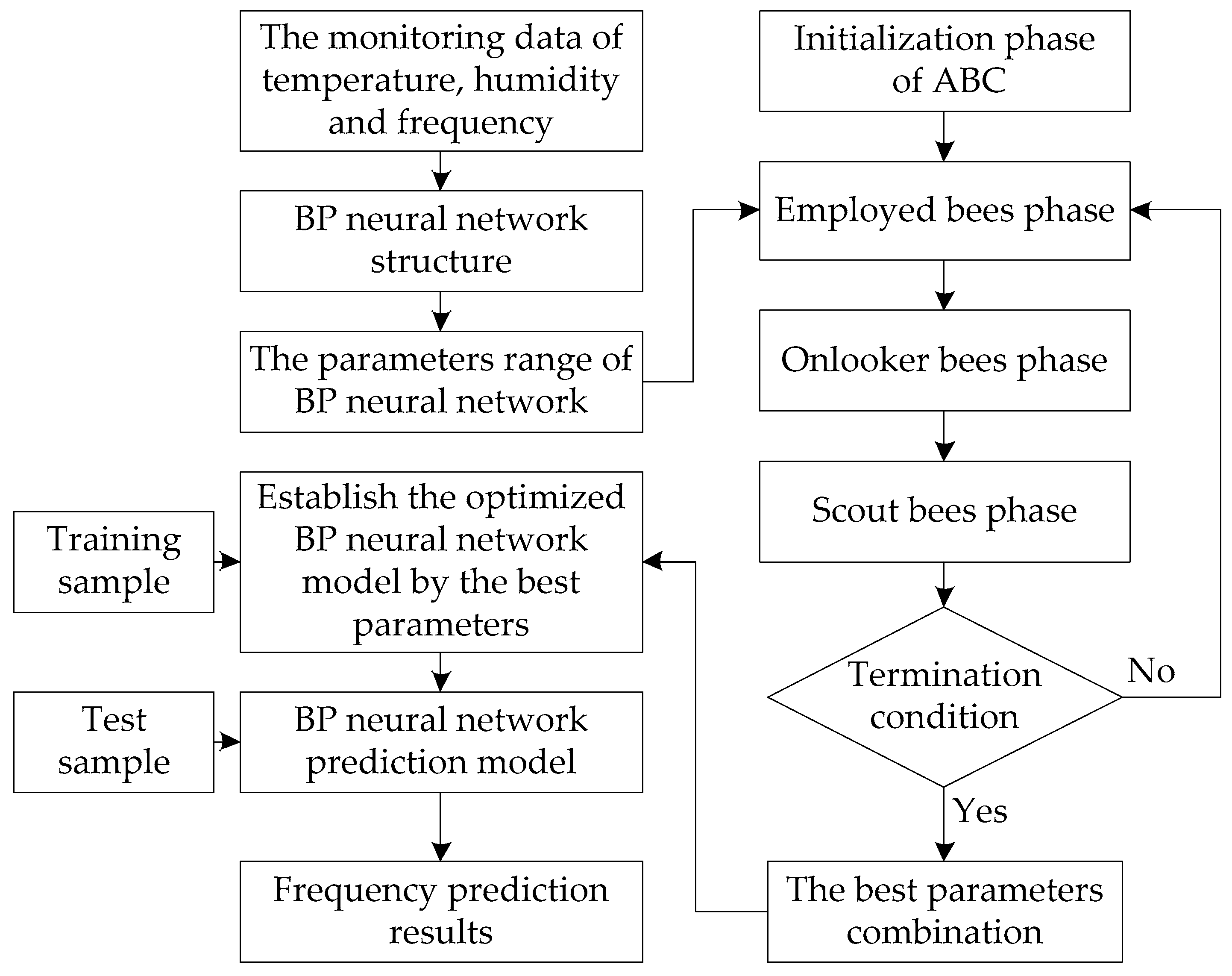
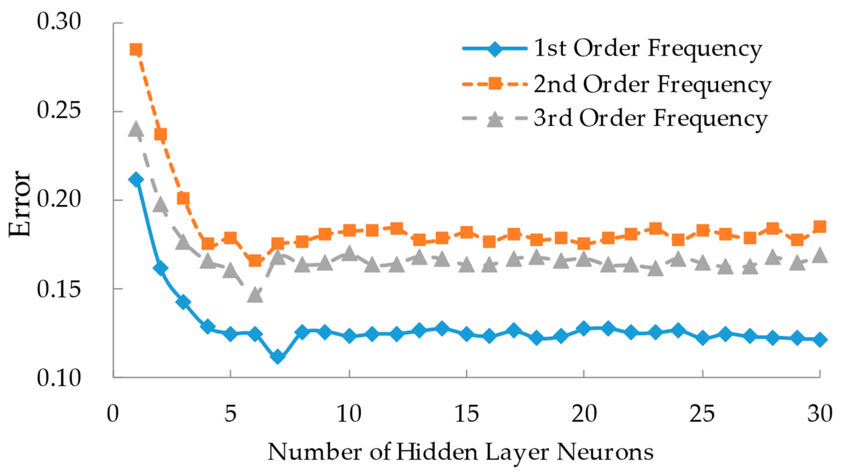
3.1. BP Neural Network

The BP neural network [42] is a multilayer feedforward network, as shown in Figure 1. The learning process consists of data forward propagation and error back propagation. The measured data is imported through the input layer, processed by the hidden layer, and exported by the output layer in the forward propagation process. If the error between the output result and the expected result do not meet the requirements, the error back propagation is carried out. At the same time, the error propagates from the output layer to the input layer and modifies the weights and thresholds of each neuron. The process of data forward propagation and error back propagation continuously alternates. When the error is less than the allowable value, or if it reaches the termination condition, it stops the neural network training process. The trained network can be used for prediction based on the measured data.

3.2. Artificial Bee Colony Algorithm

The artificial bee colony algorithm (ABC) is an optimization algorithm that simulates the process of bee foraging to find the optimal solution, which consists of four stages: initialization stage, employed bees phase, onlooker bees phase, and scout bees phase. Compared with genetic algorithm (GA), particle swarm optimization algorithm (PSO), and other swarm intelligence optimization algorithms, the ABC algorithm has the advantages of simple structure, a strong ability to search for global optimal solutions, and is easy to implement [43,44]. The main steps of the ABC algorithm are summarized as follows:

(1)

Initialization phase

Firstly, the initial food source is generated according to Equation (11), and then the adaptive value is calculated through Equation (12) to evaluate the quality of the food source.

$${\theta }_{ij}=l{b}_j+\left(u{b}_j-l{b}_j\right)\cdot rand\left(0,1\right),$$

(11)

where ${\theta }_{ij}$ is the jth parameter of the ith solution; $l{b}_j$ and $u{b}_j$ are the lower and upper bounds of the jth parameter, respectively; $rand\left(0,1\right)$ represents a randomly generated real number between 0 and 1.

$$fi{t}_i=\left\{\begin{array}{c}\frac{1}{1+f\left({\theta }_i\right)}\\ 1+abs\left(f\left({\theta }_i\right)\right)\end{array}\right.\hspace{1em}\begin{array}{c}iff({\theta }_i)\ge 0\hfill \\ otherwise\hfill \end{array},$$

(12)

where $fi{t}_i$ is the fitness of the ith solution; $f\left({\theta }_i\right)$ is the target function value of the food source ${\theta }_i$.

(2)

Employed bees phase

The employed bee will search for nearby food sources, and the forger bee corresponding to the ith food source selects a new food source according to Equation (13) and retains a better solution according to the greedy selection mechanism.

$$v_{ij}={\theta }_{ij}+{\psi }_{ij}\cdot \left({\theta }_{ij}-{\theta }_{kj}\right),$$

(13)

where $v_{ij}$ is the jth parameter corresponding to the ith new solution; ${\theta }_{ij}$ is a randomly selected food source, $k\ne i$; ${\psi }_{ij}$ is random number on interval [–1, 1].

(3)

Onlooker bees phase

The employed bees share the information of the food source with the onlooker bees after returning to the nest, and the onlooker bees select the food source according to the probability obtained by Equation (14). The best food source will be further exploited and utilized by the onlooker bees.

$$p_i=\frac{fi{t}_i}{{\displaystyle \sum _{j=1}^{FN}fi{t}_j}}.$$

(14)

(4)

Scout bees phase

If the exploitation number of a food source is more than the control parameter, it indicates that the food source is exhausted. The employed bees will be converted to scout bees and start to search for food sources randomly. The scout bee will turn back to the employed bee when it discovers a new food source, and the counter is reset to 0. The algorithm repeats from Step 2 to Step 4 until the termination condition is satisfied.

3.3. BP Neural Network Optimized by ABC Algorithm

The fitting accuracy of the BP neural network is mainly influenced by the number of hidden layer neurons, network weight, threshold, and other parameters. The BP neural network model in this paper is constructed with the bridge internal temperature, environmental temperature, and humidity as the input parameters and the modal frequency as the output parameter. The fitting function of the ABC algorithm is the Euclidean distance between the frequency predicted by the BP neural network and the frequency SHM data. The frequency SHM data cover the first three order frequencies. Therefore, three BP neural networks for the first three frequencies in this work are established. The parameters of the BP neural network are regarded as the food source in the ABC algorithm. The quality of the food source is determined by the fitting function. Through the employed bees phase, onlooker bees phase, and scout bees phase, the best combination of the parameter of the BP neural network can be obtained. Considering the efficiency and accuracy of the optimization process, the population size, iteration times, and exploitation limit of the ABC algorithm, and the upper and lower bounds of the parameters, are determined according to reference [36]. When the parameters’ combination of neurons number, network weight, and threshold are optimized by the ABC algorithm, the BP neural network model with the best accuracy can be obtained. The calculation flow of the BP neural network optimized by the ABC algorithm is shown in Figure 2.

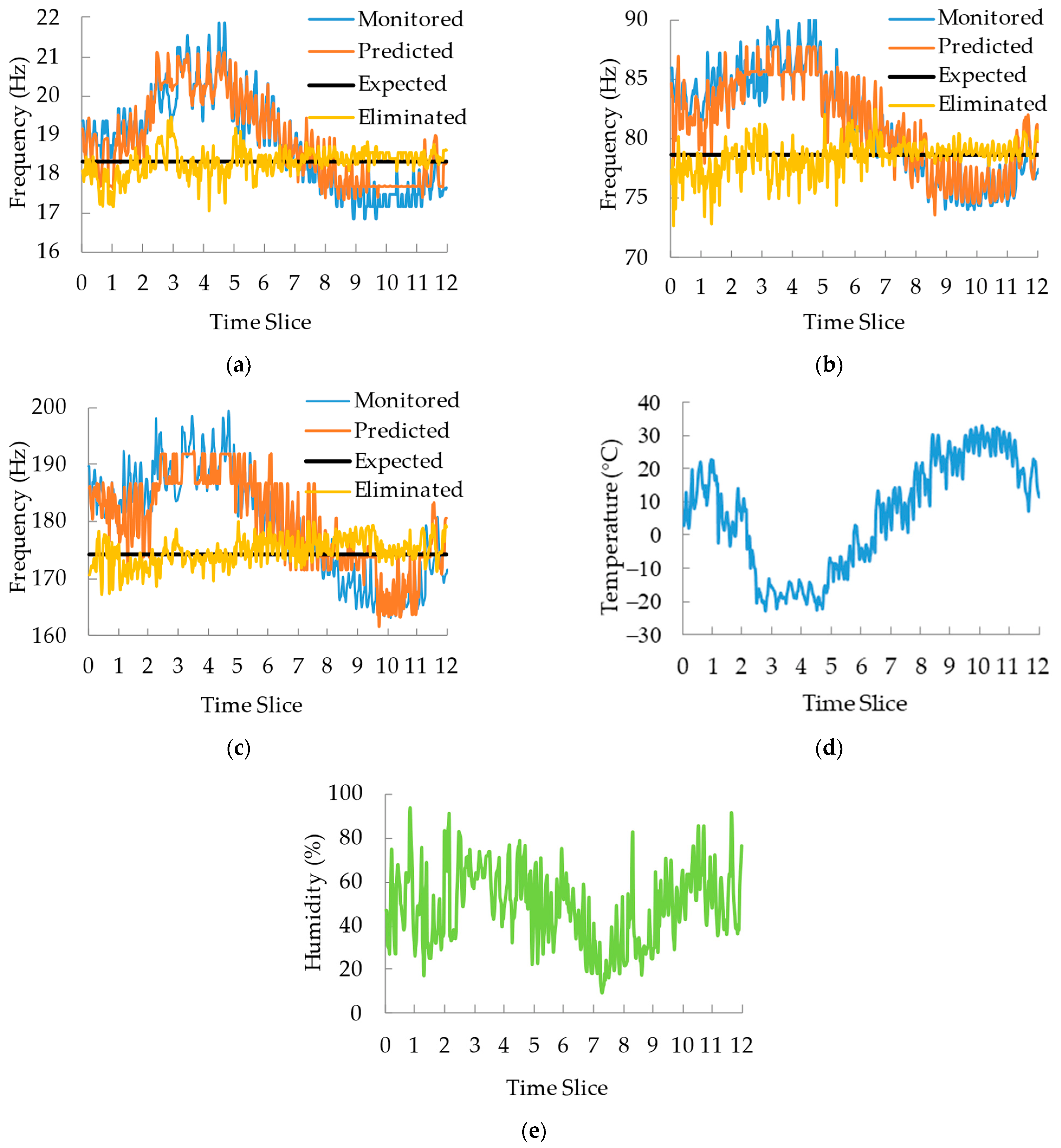
3.4. Temperature and Humidity Effect Elimination of Bridge Modal Frequency

The optimized BP neural network model is used to analyze the temperature and humidity effect on bridge frequency. The difference between the predicted frequency and the measured frequency at the reference temperature is taken as the temperature and humidity effect, which is eliminated from the measured frequency to obtain the modal frequency without the effect of temperature and humidity. It is defined as Equation (15) [45].

$$f_q=f_m-\left[f_p-f_e\right],$$

(15)

where $f_q$ is modal frequency (Hz) with temperature effect eliminated; $f_m$ is the measured frequency value (Hz); $f_p$ is the frequency value (Hz) predicted by the optimized BP neural network model; $f_e$ is the expected value (Hz) of bridge modal frequency.

In addition, the prediction capacity of the BP neural network is related to the amount of frequency SHM data. As for the SHM of the actual bridge, it can provide a sufficient measured data, which can improve the prediction accuracy of the BP neural network optimized by the ABC algorithm. Therefore, the effect of temperature and humidity on frequency can be eliminated effectively for actual bridge engineering.

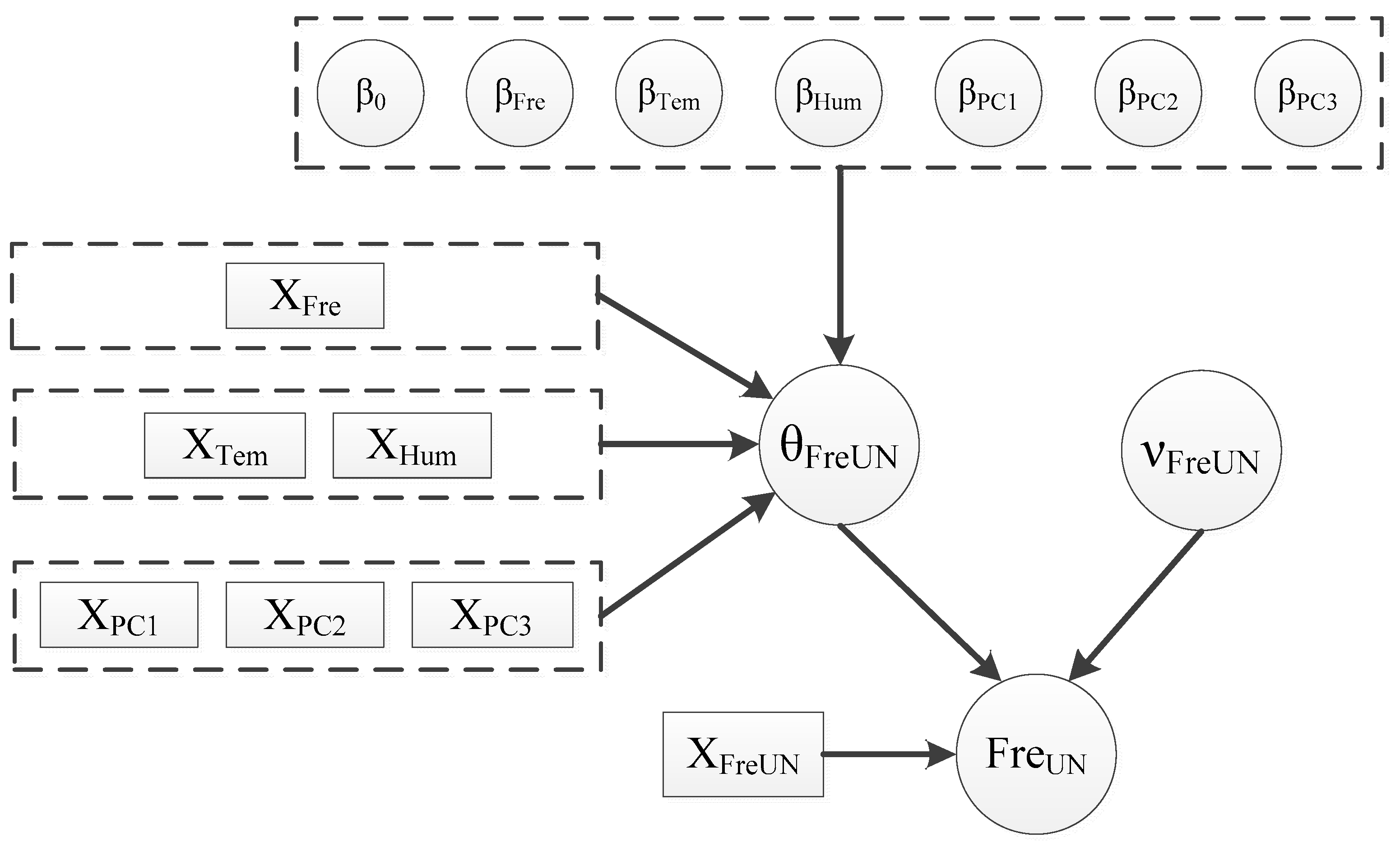
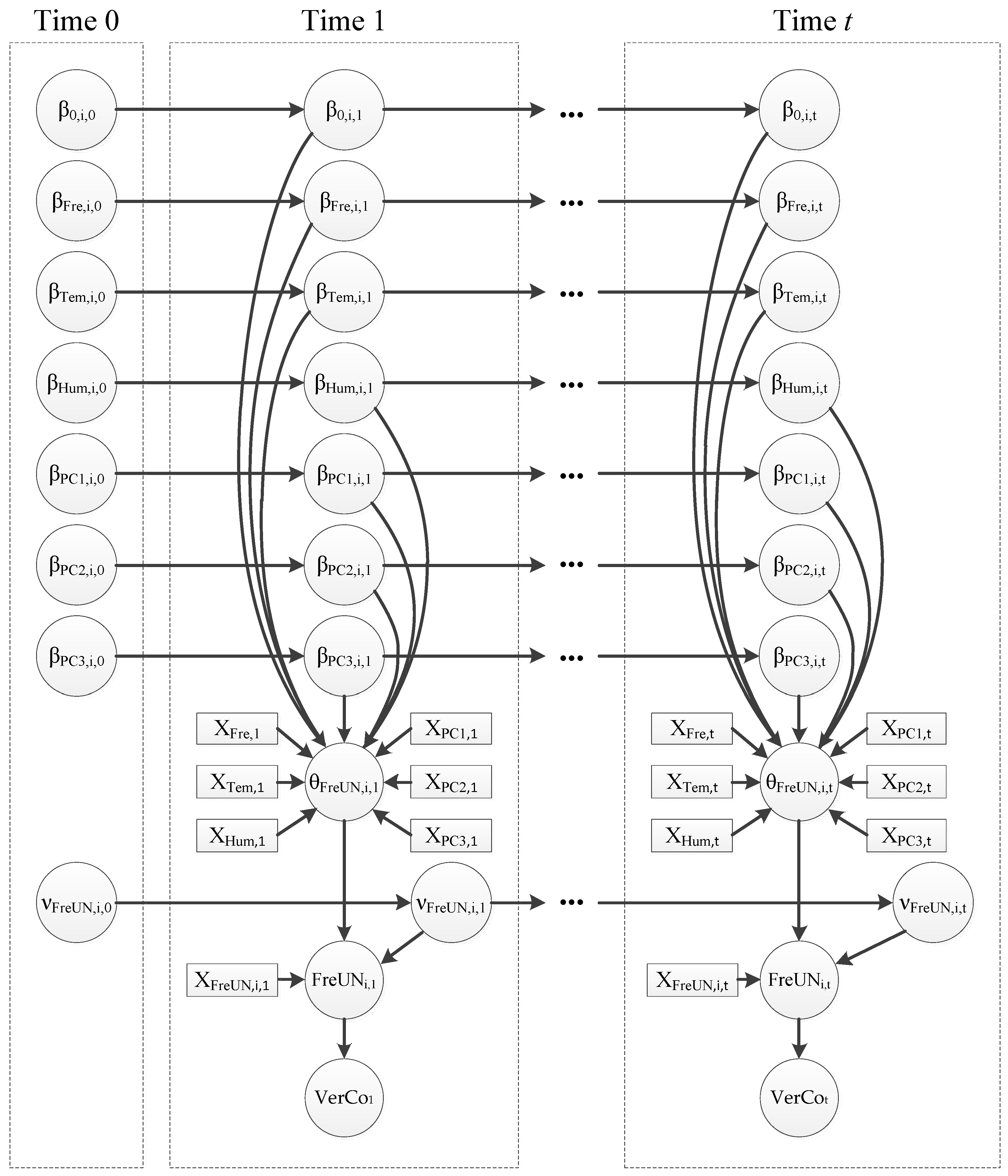
4. Dynamic Bayesian Network Model

Based on the dynamic Bayesian network, the posterior distribution of bridge frequency with the temperature and humidity effect eliminated is shown as Equation (16).

$$f\left(Fr{e}_{UN}|X\right)=\frac{L\left(X|Fr{e}_{UN}\right)\pi \left(Fr{e}_{UN}\right)}{{\displaystyle \underset{\mathsf{\Omega }}{\int }L\left(X|Fr{e}_{UN}\right)dFr{e}_{UN}}},$$

(16)

where $X={\left[X_{Fre},X_{Tem},X_{Hum},X_{PC1},X_{PC2},X_{PC3}\right]}^T$ represents the SHM data of the frequency, environmental temperature, humidity, and the internal temperature principal components; $L\left(X|Fr{e}_{UN}\right)$ is likelihood function; $\pi \left(Fr{e}_{UN}\right)$ is the prior distribution of modal frequency with the effect of factors eliminated; $\mathsf{\Omega }$ is the parameter space of $Fr{e}_{UN}$.

Equation (16) can be expressed by a statistical model, which is composed of response variables, explanatory variables, and likelihood relations. Thus, it is shown as Equation (17).

$$Fr{e}_{UN}|X~N\left({\mu }_{Fr{e}_{UN}},{\nu }_{Fr{e}_{UN}}\right),$$

(17)

where $Fr{e}_{UN}$ is the response variable; $X$ is the explanatory variable as the non-statistical part. This paper assumes that the response variable $Fr{e}_{UN}$ obeys a normal distribution of expected value ${\mu }_{Fr{e}_{UN}}$ and standard deviation ${\nu }_{Fr{e}_{UN}}$ [36].

Generally, likelihood relation can be defined as a generalized linear model and nonlinear model [36,46], while the generalized linear model has a simple structure and high applicability. Therefore, the linear model is adopted in this paper to establish the linear regression model, with response variables and explanatory variables given. The mean value of this model is equal to the expected value of the posterior distribution, therefore it can be obtained as Equation (18).

$$E\left(Fr{e}_{UN}|X\right)={\mu }_{Fr{e}_{UN}}={\beta }_0+\mathbf{\beta }X,$$

(18)

where ${\beta }_0$ is the constant coefficient of the regression model; $\mathbf{\beta }=\left[{\beta }_{Fre},{\beta }_{Tem},{\beta }_{Hum},{\beta }_{PC1},{\beta }_{PC2},{\beta }_{PC3}\right]$ represents regression parameters corresponding to each explanatory variable.

In addition to the relationship between the various SHM parameters of the bridge, the SHM parameters also possess time property. The linear model mentioned above is no longer applicable. However, the dynamic Bayesian network model can effectively solve such problems, which is a directed acyclic graph (DAG). The nodes of the DAG represent variables, and arrows represent the relationships between variables. The static simplified model among variables in this paper is shown in Figure 3, where circular nodes and rectangular nodes represent random variables and SHM data, respectively.

In order to analyze the dynamic Bayesian network model, the relationship between variables and time-dependent characteristics should first be simplified. This kind of model satisfies the characteristics of the Markov chain. Therefore, it can be assumed that the probability distribution of any time slice t is only related to the adjacent previous time slice t−1. The conditional probabilities of adjacent moments are homogeneous, and the transition probability $P\left(S_{t+1}|S_t\right)$ does not depend on time t. In addition, the dynamic Bayesian network can be divided into prior network $N_0$ and transfer network $N_{\to }$. As a result, the joint probability of all time slices can be expressed as Equation (19).

$$P\left(S_0,S_1,\cdots ,S_T\right)=P_{N_0}\left(S_0\right){\displaystyle \prod _{t=0}^T{P}_{N_{\to }}\left(S_{t+1}|S_t\right)},$$

(19)

where $S_t=\left[V_{1,t},V_{2,t},\cdots V_{n,t}\right]$ is the set of variables in time slice t.

Then, the joint probability of any node in the dynamic Bayesian network model is shown as Equation (20).

$$P\left(X_{1:n,0:T}\right)={\displaystyle \prod _{i=1}^n{P}_{N_0}\left(V_{i,0}|Pa\left(V_{i,0}\right)\right)}{\displaystyle \prod _{t=1}^T{\displaystyle \prod _{i=1}^n{P}_{N_{\to }}\left(V_{i,t}|Pa\left(V_{i,t}\right)\right)}},$$

(20)

where $Pa\left(V_{i,t}\right)$ represents the father node of the ith variable at time t.

The node $VerCo$ is calculated by Equation (10) according to the result of node $Fr{e}_{UN}$. Therefore, the dynamic Bayesian network model of the bridge verification coefficient based on SHM is shown in Figure 4. WinBUGS software is employed in this paper to calculate and analyze the dynamic Bayesian network model.

5. Experimental Test

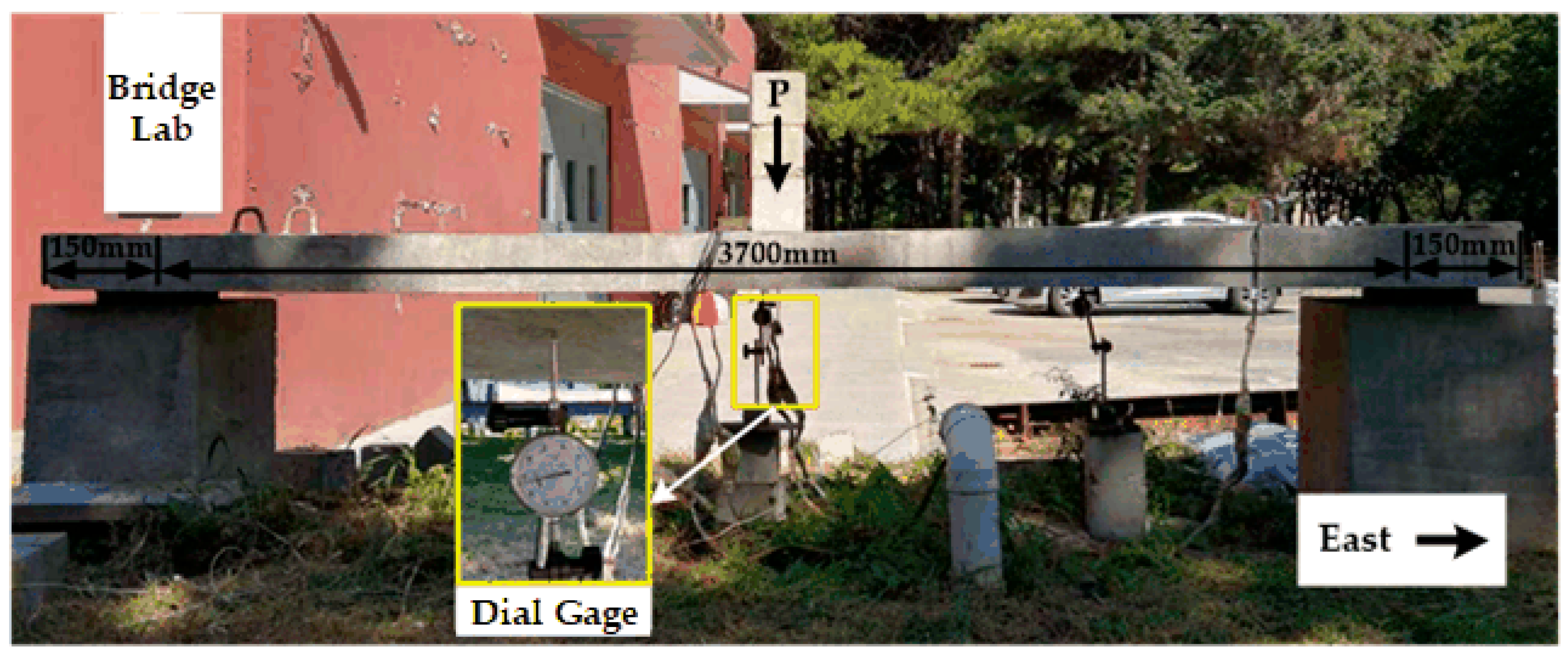
5.1. Simply Supported Bridge

In this paper, a simply supported bridge was established in the laboratory as the research object (as shown in Figure 5). The bridge is 4 m long, the calculated span is 3.7 m long, and the cross-section is a rectangle with a width of 0.6 m and a height of 0.15 m. Portland cement of grade 42.5, river sand with fineness modulus of 2.7, and aggregate with maximum nominal size of 31.5 mm were used for bridge construction. The mix proportions are illustrated in

Table 1. Mix proportions of the bridge.

Material	Unit	Proportions
Cement	kg/m3	378
Coarse aggregate	kg/m3	1230
Fine aggregate	kg/m3	607
Water	kg/m3	185
Water/cement ratio	—	0.49

. There are 6 × Φ12 steel reinforcements longitudinally arranged in the beam, and the concrete cover thickness is 4 mm. The beam is simply supported on concrete piers by plate rubber supports. The deflection verification coefficient of the simply supported bridge was obtained through the static load test. The load level of the static load test was divided into four grades, namely if the load P equals 0.5 kN, 1.0 kN, 1.5 kN, and 2.0 kN, respectively. The deflection at the midspan of four load conditions was measured by the dial gage.

5.2. Structural Health Monitoring System

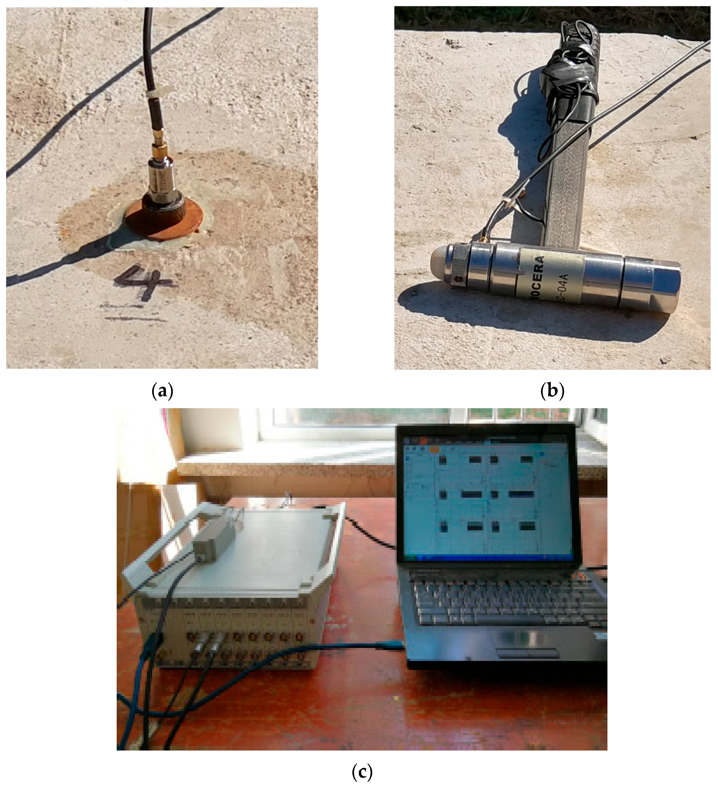
5.2.1. Modal Frequency Monitoring System

In this paper, a DH5922 dynamic signal test and analysis system (as shown in Figure 6) manufactured by Donghua Testing Technology Co., Ltd. was used to monitor the modal frequency of the bridge. The test system includes a signal analysis system, DH131E acceleration sensor, and an impulse hammer with a piezoelectric force sensor. The acceleration sensor has the advantages of small size (Φ10 × 16 mm), light weight (5.5 g), and large test range (1 Hz~8000 Hz). The force hammer pressure test range is 0 kN~60 kN. The sensor and force hammer can withstand an operating temperature of −40 °C to 80 °C and meet the field experimental environmental conditions. The dynamic test system includes two modal analysis test modes, which are force measurement method and no-force measurement method. Because the force-measured method possesses better performance and accuracy, it was used to collect and analyze the modal frequency to validate the effectiveness and accuracy of the verification coefficient method proposed in this study. Through the Modal Analysis Module in the DH5922 dynamic signal test and analysis system, it can measure the frequency more accurately, of which the frequency resolution was 0.001 Hz.

Due to the complex testing process of the force-measured method, it is not suitable for the SHM of bridge frequency. The spectral analysis was employed for the frequency SHM, which was excited by rubber hammer. The accelerometer was used to monitor vibration. The sampling frequency was set as 5120 Hz. The rectangular window was used, and the frequency resolution was 0.156 Hz. The bridge frequencies were calculated and extracted by frequency spectral analysis using fast Fourier transform. The monitoring test was carried out from October 2015 to September 2016, and the modal test was performed to measure the bridge frequencies every two hours from 8:00 a.m. to 10:00 p.m. on every day of monitoring.

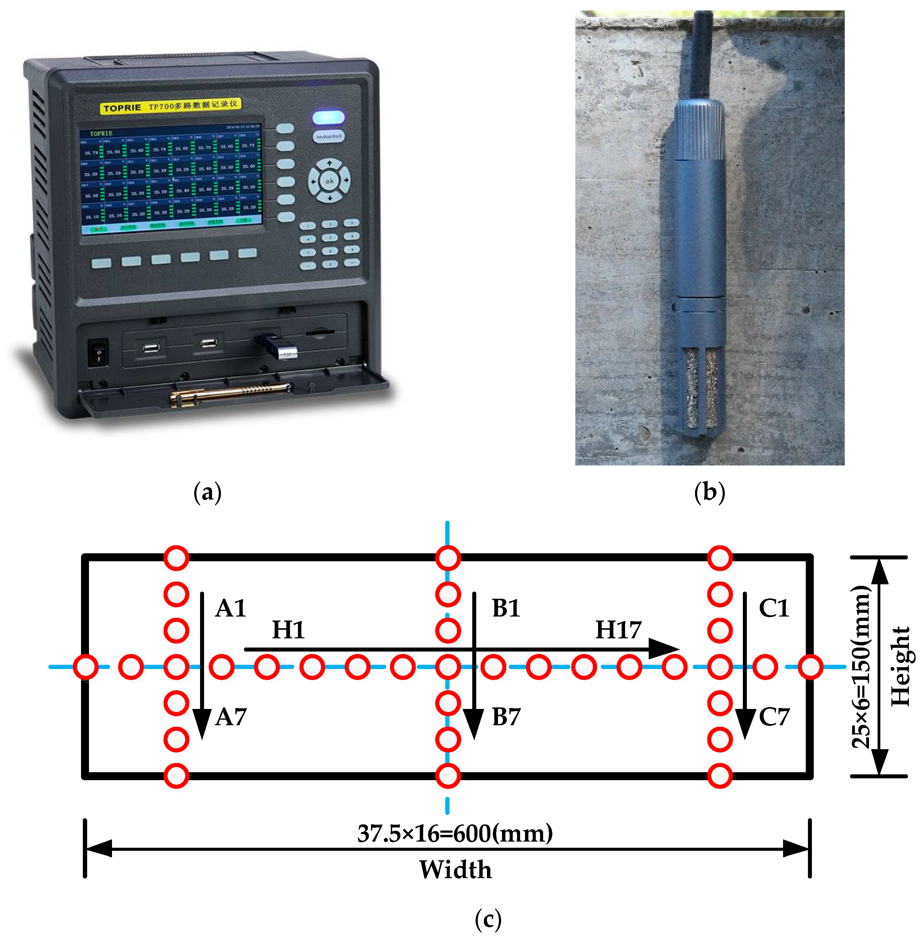
5.2.2. Temperature and Humidity Monitoring System

The temperature and humidity monitoring system manufactured by Shenzhen TOPRIE Electronics Co., Ltd. (Shenzhen, China) Was used to monitor the ambient temperature and humidity of the bridge and the bridge’s internal temperature. The system is composed of a TP-2307 digital temperature and humidity sensor and a TP700 multi-channel data recorder with a temperature and humidity input module, as shown in Figure 7a,b. The temperature measurement ranges of the temperature and humidity sensor are −40 °C ~125 °C and 0% to 99%, respectively. The temperature resolution is 0.3 °C, and the humidity resolution is 0.3%.

Omega T-type thermocouple was used to test the internal temperature of the bridge. The two poles of the Omega T-type thermocouple are composed of copper-constantan. According to the Seebeck effect, the temperature of the measuring point was measured through the thermoelectric electromotive generated in the circuit. The temperature measurement range omega T-type thermocouple is −250 °C to 260 °C. Next, 38 measuring points were arranged at the midspan cross-section of the bridge, and one thermocouple was buried at each measuring point. The layout is shown in Figure 7b.

6. Results and Discussion

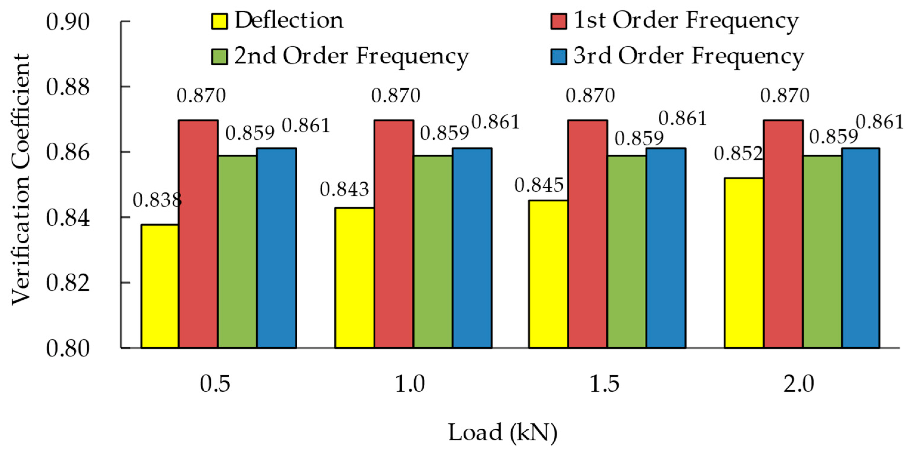
6.1. Validation of Bridge Verification Coefficient Based on Modal Frequency

The deflection values of the mid-span section of the simply supported bridge and the first three modal frequencies were obtained through static and dynamic load tests. The temperature and humidity of the field test condition were 13.3 °C and 33.7%. The results were used to verify the effectiveness and accuracy of the method proposed in this paper, which is used for calculating the bridge verification coefficient based on modal frequency, and the bridge deflections and frequencies were measured for four times to reduce the influence of a test error. Then, the corresponding theoretical values were obtained through a finite element model established by ANSYS software. The theoretical values and actual test results are shown in

Table 2. The theoretical values and measured values of deflections.

Load P Level (kN)	Theoretical Values (mm)	Measured Values (mm)
		1	2	3	4	Mean	Coefficient of Variation
0.5	0.111	0.10	0.10	0.09	0.08	0.093	0.1035
1.0	0.223	0.17	0.20	0.19	0.19	0.188	0.0671
1.5	0.329	0.26	0.29	0.28	0.28	0.278	0.0453
2.0	0.432	0.35	0.37	0.38	0.37	0.368	0.0342

and

Table 3. The theoretical values and measured values of the first three order frequencies.

Modal Order	Theoretical Values (Hz)	Measured Values (Hz)
		1	2	3	4	Mean	Coefficient of Variation
1st order	18.304	19.688	19.750	19.375	19.688	19.625	0.0086
2nd order	76.617	82.511	82.900	83.132	82.133	82.669	0.0053
3rd order	174.330	187.769	188.408	188.927	186.481	187.896	0.0056

.

The mean values and theoretical values of the measured data were substituted into Equation (2) to calculate the deflection verification coefficients of the simply supported bridge, and the deflection verification coefficients based on modal frequencies were calculated according to Equation (10). The calculation results are shown in Figure 8.

It can be seen from Table 2 that the COVs of the measured deflections of the bridge are between 0.03 and 0.1, which indicates that the static load test can provide accurate deflection values. The measured data in Table 3 were extracted and obtained through the Modal Analysis Module in the DH5922 system. The frequency resolution of this method is 0.001 Hz, and it can measure the bridge frequencies more accurately. However, the test process is influenced by the electrical interference and human factor, which leads to frequency variation between tests, and the modal test was controlled strictly in this study to reduce the error caused by the adverse factors. The COVs of the measured frequencies in Table 3 do not exceed 0.01, which demonstrates that the dynamic test has higher accuracy and reliability. In Figure 8, the results of the deflection verification coefficient calculated by the two methods are between 0.838 and 0.87, and the maximum relative error is 3.82%. This verifies the effectiveness and accuracy of the bridge deflection verification coefficient calculation method based on modal frequency. It proves that the first three modal frequencies can be used to calculate the bridge deflection verification coefficient. With an increase in static load, the deflection verification coefficients increase slightly. With an increase in modal frequency orders, the deflection verification coefficients calculated by the method proposed in this paper decrease from 0.87 to 0.859.

6.2. Bridge Frequency with the Effect of Temperature and Humidity Eliminated

The temperature data of 38 measuring points inside the bridge were obtained from the structural health monitoring system established in this paper. Due to the high correlations between the internal temperature data, there will be unstable fitting parameter estimations in the temperature effect elimination and dynamic Bayesian network analysis. The principal component analysis method was used to process the temperature-monitoring data inside the bridge. The principal analysis is an approach for linear data visualization and reduction. The principal components obtained by the principal component analysis method are numerical and contain most of the information of the original data and describe the maximum and minimum variability in the data set [47]. Moreover, the obtained temperature principal components can improve the generalization performance of the fitting model, avoiding the over-fitting phenomenon caused by information overlap. The principal component analysis was mainly calculated and analyzed according to Equations (21) and (22):

$$\mathit{Y}={\mathit{\Psi }}^T\mathit{X}={\left[y_1,y_2,\cdots ,y_n\right]}^T,$$

(21)

where $\mathit{Y}$ is principal component vector; $\mathit{X}$ is the original data vector; ${\mathit{\Psi }}^T$ is orthogonal transformation matrix, namely ${\mathit{\Psi }}^T={\mathit{\Psi }}^{-1}$. Through the singular value decomposition of the covariance matrix of $\mathit{X}$, it can be expressed as Equation (22).

$$\mathit{\Lambda }=diag\left({\lambda }_1,{\lambda }_2,\cdots ,{\lambda }_n\right),$$

(22)

where $\mathit{\Lambda }$ is a diagonal matrix composed of n eigenvalues; the eigenvalues satisfy ${\lambda }_1\ge {\lambda }_2\ge \cdots \ge {\lambda }_n\ge 0$; ${\lambda }_i$ is the contribution rate of the ith principal component. The selected principal component must meet the condition that the cumulative contribution rate is more than 85%.

The cumulative contribution rates of the principal components of the bridge’s internal temperature are shown in Figure 9. The contribution rate of the first principal component is 97.12%, which indicates that the temperature data obtained from the test have a significant correlation. Moreover, the cumulative contribution rate of the first three principal components is 99.8%, therefore it can fully characterize the information of the original internal temperature-monitoring data. The essence of the first three components is the reconstruction of the original temperature-monitoring data, which cover the monitoring data information with a smaller data size. Therefore, the first three principal components were used for analysis in the BP neural network and the dynamic Bayesian network model.

The environment temperature, humidity, and the first three principal components of bridge internal temperature were taken as the input parameters of the BP neural network model. The first three order frequencies of the SHM data of the simply supported bridge were taken as the output parameters. A total of 521 groups of monitoring data were collected by the SHM system, in which the first 417 groups of data were used as training samples and the last 104 groups of data were used as test samples. The monitoring process lasted from October 2015 to September 2016, and the modal frequency, temperature, and humidity monitoring test was preformed every two hours from 8:00 a.m. to 10:00 p.m. for every day of monitoring. The duration of a single monitoring process was 15 min. According to the temperature-monitoring data, the change of the internal temperature lags behind that of the environment temperature. Before 2:00 p.m., the environment temperature is greater than the internal temperature by about 1 °C to 4 °C. After 2:00 p.m., the environment temperature is less than the internal temperature by about 1 °C to 6 °C. The BP neural network model used in this paper has a three-layer structure, including an input layer, hidden layer, and output layer. According to the process shown in Figure 1, the bridge frequencies under the influence of temperature and humidity were fitted and predicted. The population size, iteration times, and exploitation limit of the ABC algorithm were set to 30, 300, and 150, respectively. Finally, the parameters’ combination of the hidden layer neurons number, inter layer weights, thresholds, and other parameters in the BP neural network were optimized by the ABC algorithm. The fitting error results of the optimized BP neural network are shown in Figure 10.

It can be seen from Figure 10 that the fitting errors of the first three frequencies of the bridge decrease gradually with an increase in the hidden layer neurons number. When the number of neurons is 7, the fitting error of the first order frequency reaches the minimum value. Then, the fitting error fluctuates slightly with an increase in the neurons number, and the minimum values of the fitting errors of the second and third order frequencies occur when the number of neurons in the hidden layer is 6. Therefore, the number of hidden layer neurons in the BP neural network models, for the first three order frequencies in the monitoring data, were set to 7, 6, and 6, and the optimized BP neural network model was established according to the optimal combination of layer weights, thresholds, and other parameters determined by the ABC algorithm. The predicted value, expected value, and monitored value of the SHM data were substituted into Equation (15) to calculate the first three frequencies of the simply supported slab bridge, eliminating the influence of temperature and humidity, as shown in Figure 11.

As shown in Figure 11, the monitoring temperature minimum and maximum values are in time slice 4 and time slice 10, respectively. At the same time, the corresponding frequency monitoring values are maximum and minimum, respectively. The overall change trend shows that the bridge frequency monitoring data has a negative correlation with the temperature. However, the monitoring humidity has little impact on the frequency change trend. The predicted value of the bridge frequencies is consistent with the monitored values, which shows that the BP neural network optimized by the ABC algorithm can accurately predict the bridge frequency. The frequencies with the effect of temperature and humidity eliminated will no longer vary with the change of temperature, which is closer to the expected value. Due to the influence of the test errors, human factors, and other interference factors, the frequencies with the effect of temperature and humidity eliminated fluctuate slightly around the expected value.

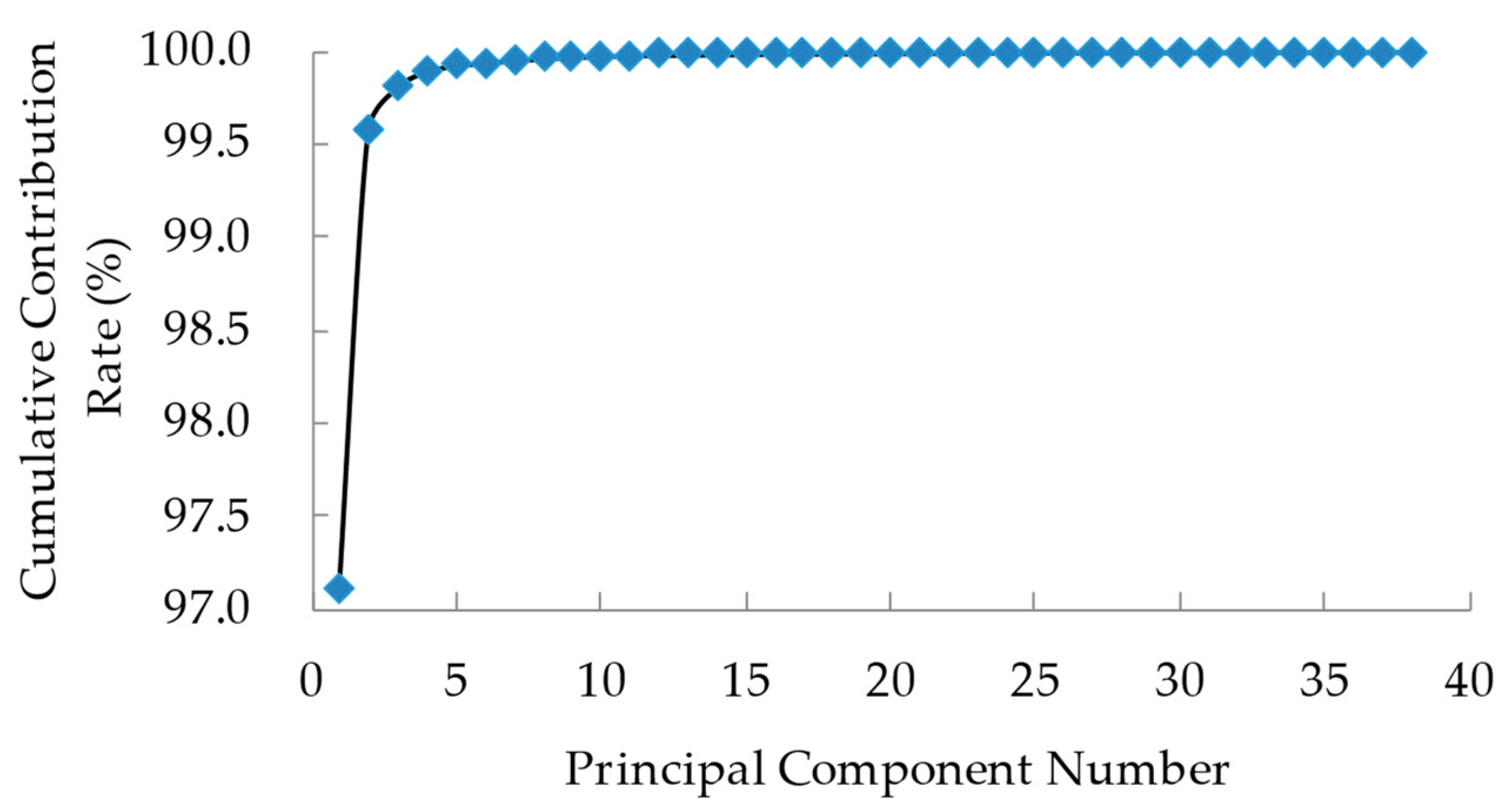
6.3. Dynamic Bayesian Network Analysis

Using the dynamic Bayesian network established above, the uncertainty of SHM data and bridge frequency with the effect of temperature and humidity eliminated were analyzed. The relationship between the monitoring variables was established through Equation (18). In this study, the SHM of the bridge was carried out from October 2015 to September 2016. The SHM data in a month were analyzed and used for a time slice of dynamic Bayesian network, and the time slice 1 to the time slice 12 corresponded to October 2015 to September 2016, respectively. According to the characteristics of the monitoring data parameters [48], this paper assumed that the regression coefficient $\beta$ and the mean value of the bridge frequency with the effect of temperature and humidity eliminated obey the normal distribution and that the standard deviation variable $\nu$ obeys the gamma distribution. For time slice 1, it was regarded as non-prior information, and the prior distribution mean and standard deviation of each variable are 0 and 10⁴, so as to reduce the influence of prior information. The WinBUGS software was adopted to calculate the posterior distribution of the first three frequencies eliminating the effect of temperature and humidity. A part of the posterior information results is shown in

Table 4. Posterior distribution information of the dynamic Bayesian network.

Variables	First Order		Second Order		Third Order		Distribution Type
	Mean Value	Standard Deviation	Mean Value	Standard Deviation	Mean Value	Standard Deviation
${\beta }_0$	34.5100	2.8180	146.400	25.5500	240.5000	37.4600	Normal istribution
${\beta }_{Fre}$	−0.8250	0.1478	−0.8431	0.3032	−0.3431	0.2026
${\beta }_{Tem}$	−0.0093	0.0101	−0.0526	0.0508	−0.1116	0.1020
${\beta }_{Hum}$	0.0021	0.0018	0.0229	0.0095	−0.0138	0.0188
${\beta }_{PC1}$	−0.0995	0.0321	−0.9589	0.1973	0.1528	0.3525
${\beta }_{PC2}$	2.7850	1.9560	−52.5800	9.6580	22.8300	19.2700
${\beta }_{PC3}$	−0.2917	0.1678	−0.9816	0.8333	−5.7380	1.6160
${\theta }_{FreUN}$	18.4800	0.0250	78.3200	0.1241	176.2000	0.2494
${\nu }_{FreUN}$	0.2218	0.0193	1.0990	0.0956	2.2080	0.1934	Gamma distribution

.

The Markov chain error of each variable in the dynamic Bayesian network is less than 1/20 of the posterior standard deviation, which indicates that the dynamic Bayesian network model is convergent and has a high accuracy [36]. Through the K–S hypothesis test, it demonstrated that the posterior distribution of each variable was the same as the prior distribution. It can be seen from Table 4 that, except for the constant term coefficient ${\beta }_0$ and the second principal component coefficient of internal temperature ${\beta }_{PC2}$, other regression coefficients have small standard deviations. Thus, the relationships between the first three order modal frequencies with the effect of temperature and humidity eliminated and the SHM parameters are expressed from Equation (23) to Equation (25).

$$\begin{array}{c}FreU{N}_{1,1}=34.51-0.825X_{Fre}-0.0093X_{Tem}+0.0021X_{Hum}\\ -0.0995X_{PC1}+2.785X_{PC2}-0.2917X_{PC3}\end{array}$$

(23)

$$\begin{array}{c}FreU{N}_{2,1}=146.4-0.8431X_{Fre}-0.0526X_{Tem}+0.0229X_{Hum}\\ -0.9589X_{PC1}-52.58X_{PC2}-0.9816X_{PC3}\end{array}$$

(24)

$$\begin{array}{c}FreU{N}_{3,1}=240.5-0.3431X_{Fre}-0.1116X_{Tem}-0.0138X_{Hum}\\ +0.1528X_{PC1}+22.83X_{PC2}-5.738X_{PC3}\end{array}$$

(25)

The fitting coefficients in each time slice have similar posterior distribution parameters, and this indicates that the change trend of environmental conditions and bridge dynamic characteristics are stable during the monitoring period. Equation (23) to Equation (25) show that the internal temperature of the bridge has the highest correlation with the frequency with the effect of temperature and humidity eliminated. The second principal component of the bridge’s internal temperature has the greatest influence, and the internal temperature of the bridge will directly cause the change of the bridge frequency. The ambient temperature and humidity will also affect the bridge frequency. The influence of ambient temperature and bridge internal temperature are much greater than that of ambient humidity, which demonstrates that the change of bridge frequency is mainly affected by temperature. Therefore, a change in bridge frequency is not only related to structural performance, but also affected by environmental factors. The accuracy of bridge service condition assessment based on modal frequency will be reduced without the effect of temperature and humidity first being eliminated. According to the analysis of the dynamic Bayesian network, the probability densities of frequencies with the effects of temperature and humidity eliminated are shown in Figure 12.

It can be seen from Figure 12 that the minimum mean value and maximum standard deviation of the first three frequencies are all in time slice 1. With the monitoring time increasing, the bridge frequencies eliminating the effect of temperature and humidity gradually tend to the same posterior mean value, and their standard deviations also decrease. This indicates that the uncertainty of the bridge frequency with the effect of temperature and humidity eliminated is reduced after the dynamic Bayesian network analysis of monitoring data, which is closer to the real probability distribution parameters.

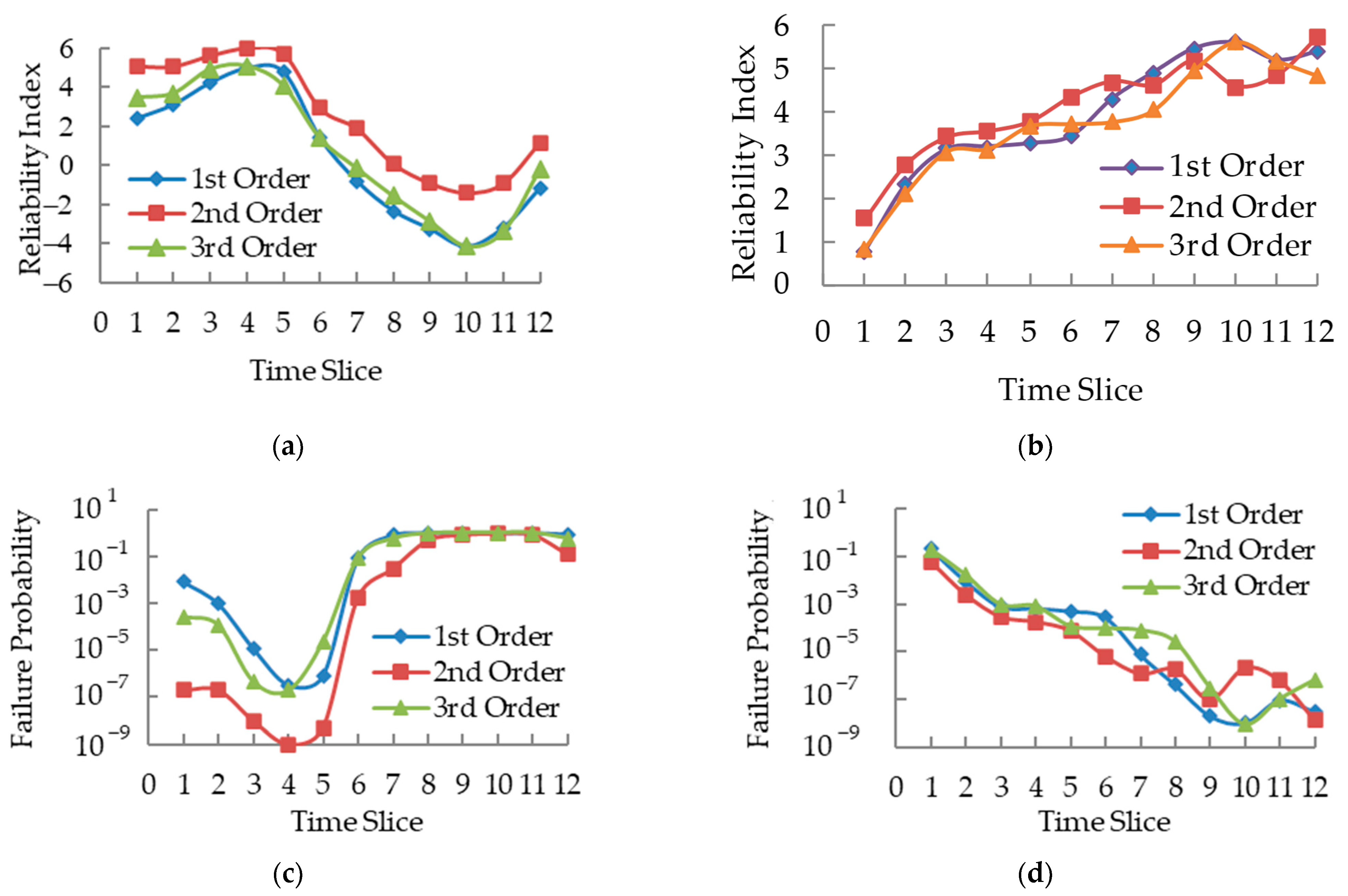
6.4. Bridge Reliability Analysis Based on Verification Coefficient

According to the Chinese specification [41], the deflection verification coefficient cannot be greater than 1, otherwise the bearing capacity of the bridge will be identified a as failure. Through the calculation method of bridge deflection verification coefficient based on modal frequency in this paper, the performance function for bridge-bearing capacity evaluation can be defined as Equation (26). The reliability is calculated and analyzed by the Monte Carlo method. According to the analysis results of the dynamic Bayesian network, this paper assumes that the mean value and the standard deviation of the bridge frequency with the effect of temperature and humidity eliminated obey the normal distribution and the gamma distribution, respectively.

$$Z=1-{\eta }_{Fre}^{-2}.$$

(26)

Then, the failure probability and reliability index [26] are defined as:

$$FP=\mathrm{Pr}\left(Z<0\right),$$

(27)

$$RI=-{\mathsf{\Phi }}^{-1}\left[\mathrm{Pr}\left(Z<0\right)\right].$$

(28)

According to the posterior distribution information of bridge frequency after eliminating the effect of temperature and humidity, the Monte Carlo sampling method was used to calculate Equation (28). Based on the posterior distribution of the first three order frequencies, the reliability index and failure probability of the bridge-bearing capacities before and after eliminating the effect of temperature and humidity were computed and are shown in Figure 13.

According to the results shown in Figure 13, the temperature and humidity have a significant influence on the reliability evaluation of the bridge deflection verification coefficient. There is a significant difference between the reliability index before and after eliminating the effect of temperature and humidity. In Figure 13a, the reliability index without the effect of temperature and humidity eliminated is opposite to the variation trend of temperature. From the time slice 4 to 10, the reliability index values decrease from 5.99 to −4.18. The reliability index calculated by the first three order frequencies’ SHM data possess the same variation trend. The calculation results based on the first order and the third order are basically consistent, while the reliability index based on the second order is slightly higher. In Figure 13b, the variation trends of reliabilities based on the first three frequencies are consistent after the effects of temperature and humidity are eliminated. The minimum of the reliability index appears in time slice 1. As time increases, the reliability index is gradually stable at 5.1 and fluctuates slightly. As seen from Figure 13c,d, the variation trend of the failure probability differs from the change in the reliability index. Due to the influence of non-prior information in the dynamic Bayesian network, the error of the probability distribution parameters in time slice 1 is large. Therefore, the reliability index in time slice 1 is much less than those of other time slices. With the continuous updating of monitoring data, the frequency probability distribution information after eliminating the influence is closer to the real value. The bridge-bearing capacity evaluation based on reliability theory can reflect the real condition of the structure. In this paper, the monitoring data were collected in a whole year, which was from October 2015 to September 2016. Both the reliability index and failure probability were gradually stable in time slice 9 to time slice 12, and the change of the reliability results from time slice 1 to time slice 3 was influenced by the accuracy provided after temperature and humidity effect elimination. The temperature and humidity effect elimination method is related to the amount of monitoring data. If more monitoring data are obtained, the reliability results will converge to a point, which is the real reliability index and failure probability of the bridge. Taking the reliability index of time slice 10 as an example, the evaluation result indicates a failing grade when the temperature and humidity effects are not eliminated. If the effects are eliminated, the reliability result reveals that the bridge is safe and reliable. This verifies the effectiveness and accuracy of the method established in this paper.

7. Conclusions

A verification coefficient calculation method of bridge deflection was proposed based on modal frequency. As a safety indicator, it was used to evaluate bridge condition in combination with SHM techniques and reliability theory. Considering the effect of temperature and humidity on frequency monitoring data, the temperature and humidity elimination method was established based on the BP neural network, which was improved by the ABC algorithm. The dynamic Bayesian network was adopted to analyze the probabilistic distribution information of the SHM data and the frequency with the effect of temperature and humidity eliminated. This improved the reliability assessment accuracy of the bridge’s condition. The main conclusions are drawn as follows:

(1)

The relationship between modal frequency and verification coefficient was obtained through theoretical derivation. Through the comparation between static test and dynamic test, it verified the verification coefficient calculation method based on modal frequency. The results demonstrated that the verification coefficient computed by the proposed method coincided with that obtained through the static test. The first three modal of frequencies can be used for deflection verification coefficient calculation;

(2)

The BP neural network optimized by an artificial bee colony algorithm has high fitting precision, which is adopted for the influence of temperature and humidity on the monitoring frequency elimination method. The bridge frequency does not change with temperature and humidity; rather, it only fluctuates slightly near the expected frequency and gradually approaches the expected value;

(3)

According to the results analyzed using the dynamic Bayesian network, bridge internal temperature possesses the greatest influence on the bridge frequency, and ambient temperature and humidity also clearly affect the bridge frequency. However, the change of bridge frequency is mainly influenced by temperature. With more monitoring data, the posterior information of bridge frequency demonstrated that the proposed method reduced the uncertainty of bridge frequency with the temperature and humidity effect eliminated, and showed that it is closer to the real probability distribution parameter;

(4)

The bridge reliability calculation results reveal that the reliability indices have a great difference before and after the temperature and humidity effects are eliminated. When the temperature and humidity effects are eliminated, the variations of bridge reliability are independent of temperature and humidity. The bridge performance cannot be accurately estimated without the temperature and humidity effects being eliminated. The proposed method in this paper provides a new theoretical basis and technical support for bridge SHM.

References

1. Mu, H.; Zheng, Z.; Wu, X.; Su, C. Bayesian Network-Based Modal Frequency–Multiple Environmental Factors Pattern Recognition for the Xinguang Bridge Using Long-Term Monitoring Data. J. Low Freq. Noise Vib. Act. Control. 2018, 39, 545–559. [Google Scholar] [CrossRef]
2. Sun, S.; Liang, L.; Li, M.; Li, X. Bridge Performance Evaluation via Dynamic Fingerprints and Data Fusion. J. Perform. Constr. Fac. 2019, 33, 04019004. [Google Scholar] [CrossRef]
3. Hasan, S.; Elwakil, E. Knowledge-driven stochastic reliable modeling for steel bridge deck condition rating prediction. J. Struct. Integr. Main. 2021, 6, 91–98. [Google Scholar] [CrossRef]
4. Xia, Y.; Jian, X.; Yan, B.; Su, D. Infrastructure Safety Oriented Traffic Load Monitoring Using Multi-Sensor and Single Camera for Short and Medium Span Bridges. Remote Sens. 2019, 11, 2651. [Google Scholar] [CrossRef] [Green Version]
5. Lei, X.; Sun, L.; Xia, Y.; He, T. Vibration-Based Seismic Damage States Evaluation for Regional Concrete Beam Bridges Using Random Forest Method. Sustainability 2020, 12, 5106. [Google Scholar] [CrossRef]
6. Whitlow, R.D.; Haskins, R.; McComas, S.L.; Crane, C.K.; Howard, I.L.; McKenna, M.H. Remote Bridge Monitoring Using Infrasound. J. Bridge Eng. 2019, 24, 04019023. [Google Scholar] [CrossRef]
7. Feng, D.; Feng, M.Q. Experimental Validation of Cost-Effective Vision-Based Structural Health Monitoring. Mech. Syst. Signal Process. 2017, 88, 199–211. [Google Scholar] [CrossRef]
8. Prakash, G. A Deflection-Based Practicable Method for Health Monitoring of In-Service Bridges. Meas. Sci. Technol. 2021, 32, 075108. [Google Scholar] [CrossRef]
9. Farreras-Alcover, I.; Chryssanthopoulos, M.K.; Andersen, J.E. Regression Models for Structural Health Monitoring of Welded Bridge Joints Based on Temperature, Traffic and Strain Measurements. Struct. Health Monit. 2015, 14, 648–662. [Google Scholar] [CrossRef] [Green Version]
10. Pan, C.; Yu, L.; Liu, H. Identification of Moving Vehicle Forces on Bridge Structures via Moving Average Tikhonov Regularization. Smart Mater. Struct. 2017, 26, 085041. [Google Scholar] [CrossRef]
11. Seo, J.; Hu, J.W.; Lee, J. Summary Review of Structural Health Monitoring Applications for Highway Bridges. J. Perform. Constr. Fac. 2016, 30, 04015072. [Google Scholar] [CrossRef]
12. Whelan, M.J.; Gangone, M.V.; Janoyan, K.D.; Jha, R. Real-Time Wireless Vibration Monitoring for Operational Modal Analysis of An Integral Abutment Highway Bridge. Eng. Struct. 2009, 31, 2224–2235. [Google Scholar] [CrossRef]
13. Tan, C.; Uddin, N.; Obrien, E.J.; McGetrick, P.J.; Kim, C.W. Extraction of Bridge Modal Parameters Using Passing Vehicle Response. J. Bridge Eng. 2019, 24, 04019087. [Google Scholar] [CrossRef]
14. Lee, L.S.; Karbhari, V.M.; Sikorsky, C. Structural Health Monitoring of CFRP Strengthened Bridge Decks Using Ambient Vibrations. Struct. Health Monit. 2007, 6, 199–214. [Google Scholar] [CrossRef]
15. Liu, C.; DeWolf, J.T.; Kim, J.H. Development of A Baseline for Structural Health Monitoring for A Curved Post-Tensioned Concrete Box-Girder Bridge. Eng. Struct. 2009, 31, 3107–3115. [Google Scholar] [CrossRef]
16. Li, J.; Zhu, X.; Law, S.; Samali, B. Time-Varying Characteristics of Bridges under the Passage of Vehicles Using Synchroextracting Transform. Mech. Syst. Signal Process. 2020, 140, 106727. [Google Scholar] [CrossRef]
17. Nandan, H.; Singh, M.P. Effects of Thermal Environment on Structural Frequencies: Part I—A Simulation Study. Eng. Struct. 2014, 81, 480–490. [Google Scholar] [CrossRef]
18. He, H.; Wang, W.; Zhang, X. Frequency Modification of Continuous Beam Bridge Based on Co-Integration Analysis Considering the Effect of Temperature and Humidity. Struct. Health Monit. 2019, 18, 376–389. [Google Scholar] [CrossRef]
19. Xia, Y.; Xu, Y.; Wei, Z.; Zhu, H.; Zhou, X. Variation of Structural Vibration Characteristics Versus Non-Uniform Temperature Distribution. Eng. Struct. 2011, 33, 146–153. [Google Scholar] [CrossRef] [Green Version]
20. Teng, J.; Tang, D.-H.; Hu, W.; Lu, W.; Feng, Z.; Ao, C.; Liao, M. Mechanism of the Effect of Temperature on Frequency Based on Long-Term Monitoring of An Arch Bridge. Struct. Health Monit. 2021, 20, 1716–1737. [Google Scholar] [CrossRef]
21. Cai, Y.; Zhang, K.; Ye, Z.; Liu, C.; Lu, K.; Wang, L. Influence of Temperature on the Natural Vibration Characteristics of Simply Supported Reinforced Concrete Beam. Sensors 2021, 21, 4242. [Google Scholar] [CrossRef] [PubMed]
22. Kromanis, R.; Kripakaran, P. Data-Driven Approaches for Measurement Interpretation: Analysing Integrated Thermal and Vehicular Response in Bridge Structural Health Monitoring. Adv. Eng. Inform. 2017, 34, 46–59. [Google Scholar] [CrossRef] [Green Version]
23. Deng, Y.; Li, A.; Feng, D. Probabilistic Damage Detection of Long-Span Bridges Using Measured Modal Frequencies and Temperature. Int. J. Struct. Stab. Dy. 2018, 18, 1850126. [Google Scholar] [CrossRef]
24. Wang, Z.; Yi, T.; Yang, D.; Li, H.; Liu, H. Eliminating the Bridge Modal Variability Induced by Thermal Effects Using Localized Modeling Method. J. Bridge Eng. 2021, 26, 04021073. [Google Scholar] [CrossRef]
25. Gonen, S.; Soyoz, S. Reliability-based seismic performance of masonry arch bridges. Struct. Infrastruct. Eng. 2021, 2021, 1–16. [Google Scholar] [CrossRef]
26. Dissanayake, P.B.R.; Karunananda, P.A.K. Reliability Index for Structural Health Monitoring of Aging Bridges. Struct. Health Monit. 2008, 7, 175–183. [Google Scholar] [CrossRef]
27. Newhook, J.P.; Edalatmanesh, R. Integrating Reliability and Structural Health Monitoring in the Fatigue Assessment of Concrete Bridge Decks. Struct. Infrastruct. Eng. 2013, 9, 619–633. [Google Scholar] [CrossRef]
28. Kaloop, M.R.; Eldiasty, M.; Hu, J.W. Safety and Reliability Evaluations of Bridge Behaviors under Ambient Truck Loads through Structural Health Monitoring and Identification Model Approaches. Measurement 2021, 187, 110234. [Google Scholar] [CrossRef]
29. Catbas, F.N.; Susoy, M.; Frangopol, D.M. Structural health monitoring and reliability estimation: Long span truss bridge application with environmental monitoring data. Eng. Struct. 2008, 30, 2347–2359. [Google Scholar] [CrossRef]
30. Fan, X.P.; Liu, Y.F. Time-variant reliability prediction of bridge system based on BDGCM and SHM data. Struct. Control Health Monit. 2018, 25, e2185. [Google Scholar] [CrossRef]
31. Xu, X.; Ren, Y.; Huang, Q.; Zhao, D.; Tong, Z.; Chang, W. Thermal response separation for bridge long-term monitoring systems using multi-resolution wavelet-based methodologies. J. Civ. Struct. Health 2020, 10, 527–541. [Google Scholar] [CrossRef]
32. Bhattacharya, B.; Li, D.; Chajes, M.; Hastings, J. Reliability-Based Load and Resistance Factor Rating Using In-Service Data. J. Bridge Eng. 2005, 10, 530–543. [Google Scholar] [CrossRef] [Green Version]
33. Liu, Y.; Fan, X. Gaussian Copula–Bayesian Dynamic Linear Model–Based Time-Dependent Reliability Prediction of Bridge Structures Considering Nonlinear Correlation between Failure Modes. Adv. Mech. Eng. 2016, 8, 1687814016681372. [Google Scholar] [CrossRef]
34. Chen, C.; Wang, Z.; Wang, Y.; Wang, T.; Luo, Z. Reliability Assessment for PSC Box-Girder Bridges Based on SHM Strain Measurements. J. Sens. 2017, 2017, 8613659. [Google Scholar] [CrossRef] [Green Version]
35. Kaloop, M.R.; Kim, K.H.; Elbeltagi, E.; Jin, X.; Hu, J.W. Service-Life Evaluation of Existing Bridges Subjected to Static and Moving Trucks Using Structural Health Monitoring System: Case Study. KSCE J. Civ. Eng. 2020, 24, 1593–1606. [Google Scholar] [CrossRef]
36. Liu, H.; He, X.; Jiao, Y.; Wang, X. Reliability Assessment of Deflection Limit State of a Simply Supported Bridge Using Vibration Data and Dynamic Bayesian Network Inference. Sensors 2019, 19, 837. [Google Scholar] [CrossRef] [Green Version]
37. Kaloop, M.R.; Elsharawy, M.; Abdelwahed, B.; Hu, J.W.; Kim, D. Performance Assessment of Bridges Using Short-Period Structural Health Monitoring System: Sungsu Bridge Case Study. Smart Struct. Syst. 2020, 26, 667–680. [Google Scholar] [CrossRef]
38. Jamali, S.; Chan, T.H.T.; Nguyen, A.; Thambiratnam, D.P. Reliability-Based Load-Carrying Capacity Assessment of Bridges Using Structural Health Monitoring and Nonlinear Analysis. Struct. Health Monit. 2019, 18, 20–34. [Google Scholar] [CrossRef] [Green Version]
39. Gehl, P.; D’Ayala, D. Development of Bayesian Networks for the Multi-Hazard Fragility Assessment of Bridge Systems. Struct. Saf. 2016, 60, 37–46. [Google Scholar] [CrossRef]
40. Morales-Napoles, O.; Steenbergen, R.D.J.M. Analysis of Axle and Vehicle Load Properties through Bayesian Networks Based on Weigh-In-Motion Data. Reliab. Eng. Syst. Safe. 2014, 125, 153–164. [Google Scholar] [CrossRef]
41. Research Institute of Highway Ministry of Transport of China. Specification for Inspection and Evaluation of Load-Bearing Capacity of Highway Bridges, 1st ed.; China Communications Press: Beijing, China, 2011. (In Chinese)
42. Wang, X.; Miao, C.; Wang, X. Prediction analysis of deflection in the construction of composite box-girder bridge with corrugated steel webs based on MEC-BP neural networks. Structures 2021, 32, 691–700. [Google Scholar] [CrossRef]
43. Karaboga, D.; Akay, B. A comparative study of Artificial Bee Colony algorithm. Appl. Math. Comput. 2009, 214, 108–132. [Google Scholar] [CrossRef]
44. Pham, D.T.; Castellani, M. Benchmarking and comparison of nature-inspired population-based continuous optimisation algorithms. Soft Comput. 2014, 18, 871–903. [Google Scholar] [CrossRef]
45. Tan, G.; Liu, Z. Temperature Effect Analysis of Bridge Natural Frequency Based on Particle Swarm Optimized Neural Network. In Proceedings of the 7th IEEE Annual International Conference on CYBER Technology in Automation, Control and Intelligent Systems, Honolulu, HI, USA, 31 July 2017. [Google Scholar]
46. Fan, X. Bridge extreme stress prediction based on Bayesian dynamic linear models and non-uniform sampling. Struct. Health Monit. 2017, 16, 253–261. [Google Scholar] [CrossRef]
47. Sen, D.; Erazo, K.; Zhang, W.; Nagarajaiah, S.; Sun, L. On the effectiveness of principal component analysis for decoupling structural damage and environmental effects in bridge structures. J. Sound Vib. 2019, 457, 280–298. [Google Scholar] [CrossRef]
48. Ntzoufras, I. Bayesian Modeling Using WinBUGS, 1st ed.; John Wiley & Sons Publication: Hoboken, NJ, USA, 2009; pp. 151–166. [Google Scholar]
Figure 1. Structure diagram of BP neural network.
Sustainability 14 09600 g001
Figure 2. Flow chart of BP neural network model optimized by ABC algorithm.
Sustainability 14 09600 g002
Figure 3. The Bayesian network model for bridge frequency analysis with temperature and humidity eliminated.
Sustainability 14 09600 g003
Figure 4. The dynamic Bayesian network for bridge verification coefficient based on SHM data.
Sustainability 14 09600 g004
Figure 5. The simply supported bridge.
Sustainability 14 09600 g005
Figure 6. Bridge dynamic characteristic monitoring system: (a) accelerometer; (b) hammer; (c) DH5922 type dynamic test system.
Sustainability 14 09600 g006
Figure 7. Temperature and humidity monitoring system: (a) temperature and humidity recorder; (b) temperature and humidity sensor; (c) layout of temperature-monitoring sensors inside the bridge.
Sustainability 14 09600 g007
Figure 8. The deflection verification coefficients of the simply supported bridge.
Sustainability 14 09600 g008
Figure 9. Cumulative contribution rate of principal components of bridge internal temperature-monitoring data.
Sustainability 14 09600 g009
Figure 10. The relationships between the fitting error and the number of hidden layer neurons.
Sustainability 14 09600 g010
Figure 11. Bridge frequencies excluding the influence of temperature and humidity: (a) first order frequency; (b) second order frequency; (c) third order frequency; (d) monitoring data of ambient temperature; (e) monitoring data of ambient humidity.
Sustainability 14 09600 g011
Figure 12. Bridge frequency probability densities eliminating the effect of temperature and humidity: (a) first order; (b) second order; (c) third order.
Sustainability 14 09600 g012aSustainability 14 09600 g012b
Figure 13. Reliability analysis of bridge deflection verification coefficient: (a) reliability index before eliminating the temperature and humidity effect; (b) reliability index after eliminating the temperature and humidity effect; (c) failure probability before eliminating the temperature and humidity effect; (d) failure probability after eliminating the temperature and humidity effect.
Sustainability 14 09600 g013