The Effect of Energy Consumption on China’s Regional Economic Growth from a Spatial Spillover Perspective

Abstract

Under the downward pressure of the economy, China’s extensive economic growth relying on factor input is difficult to sustain, and adjusting the total amount and structure of energy consumption to promote high-quality economic development has become an urgent problem to be solved. Based on the exploratory spatial data analysis method (ESDA) and the partial differential method of the spatial regression model, the paper measures the spatial spillover effect of energy consumption on economic growth by taking 30 provincial units in China as the research object. The results are as follows: (1) There is a significant spatial agglomeration in the spatial distribution of regional economic growth and energy consumption, that a core-periphery model has been formed with the eastern region as the core. Therefore, in view of the imbalance in regional development, more attention should be paid to the rationality of industrial spatial distribution when formulating policies, so as to achieve the sustainable development of China’s economy. (2) Through further empirical testing of spatial metrology, it has been found that regional energy consumption has a significant spatial spillover effect on economic growth, and this effect varies according to region and type of energy consumption. Among them, although coal consumption accounts for the largest proportion of energy consumption structure, the economic effect is very limited, which provides a possibility for the government to optimize the allocation of energy resources and shift to a green economy. Therefore, more energy policies should be developed to encourage the development of clean energy.

1. Introduction

Energy is the material basis for the development of human society and a strategic resource for economic development. Energy consumption is one of the driving forces of economic growth [1]. Energy consumption reflects economic and social performance and, to some extent, can be considered a “simultaneous indicator” of the economic and social development of regions.

With the worldwide outbreak of the energy crisis in the 1970s, the importance of energy issues in economic development has become increasingly prominent, with most countries designating energy as an important strategic resource and incorporating it into their national security framework system [2]. Taking the BRICs as an example, as the five developing countries that have attracted much attention in the world today, rapid economic development is the common feature of the BRICs countries [3]. According to the World Economic Outlook released by the International Monetary Fund (IMF) in October 2021, the total GDP of the BRICs has increased to 31.2% in terms of purchasing power parity, accounting for nearly 1/3 of the global economy. However, the high-speed economic growth of BRICs is heavily dependent on energy consumption, research shows that the coal-oriented energy consumption structure is hard to reduce carbon emissions and improve its energy-environment efficiency. Energy-environment efficiency in Brazil is relatively higher and this country is the only one which possesses the higher GDP and the lower carbon emission among BRICS countries; India’s energy-environment efficiency is relatively stable and its average value is only higher than China [4].

As for China, over the past 40 years of the reform and opening-up, China’s energy consumption has continued to increase and now ranks first in the world in terms of total energy consumption. In 2020, the total energy consumption was 4.98 billion tons of standard coal, up to 2.2% from 2019. In the future, China’s energy demand will continue to grow with the expansion of the economic volume and the improvement of people’s material living standards, resulting in an increasingly prominent energy shortage, which means there is a long way to go to optimize the energy structure. The greenhouse gas emissions and environmental pollution caused by the long-standing rough energy consumption pattern also pose a serious challenge to the improvement of China’s environmental quality [5]. In current years, China’s energy-environment efficiency appears the ascent trend because of the reasonable implementation of energy saving and emission reduction policies and the deep exploitation of renewable energy. However, there are still dual pressures of energy resource shortage and environmental pollution in the optimization of the Chinese economic structure, and the energy consumption is becoming a constraint on the stage of high-quality development [6].

Facing the deterioration of the ecological environment and the demand for global climate governance, BRICs have also put forward their own goals of carbon neutrality or net zero emission and formulated relevant policies [7]. The Chinese government committed to peak carbon dioxide emissions before 2030 and achieve carbon neutrality before 2060 at the 75th Session of the United Nations General Assembly. The 12th Five-Year Plan has taken the development of a low-carbon economy as China’s new economic growth point. The development goals of the 14th Five-Year Plan proposed to improve the dual control of total energy consumption and intensity, accelerate the adjustment and optimization of industrial and energy structures, incorporate low-carbon development into macroeconomic governance—to eventually achieve a green transformation of production and lifestyle, as well as a rational allocation of energy resources [7,8]. The white paper “China’s Policies and Actions to Address Climate Change” proposes that China, as the world’s largest developing country, will do its utmost to address global climate change and explore a green and low-carbon development path that is consistent with China’s national conditions.

In this context, it is crucial to adjust the total amount and structure of energy consumption to match economic growth, environmental protection, and social development [1]. China is a large country with a dualistic economic structure, and there are huge differences in regional economic development levels [9]. In this context, the dependency between energy consumption and economic growth should be given constant attention. Therefore, from a spatial perspective, this paper quantifies the characteristics of energy consumption, economic growth, and the relationship between the two in each province, city, and autonomous region in China, trying to explore the impact and constraints of energy consumption on regional economic development.

This study’s main contributions are as follows: First, to fulfill the spatial correlation test, this paper uses exploratory spatial data analysis (ESDA). Specifically, we try to visually identify the spatial differences and agglomeration characteristics of energy consumption and economic growth in various regions of China through the spatial pattern map and Lisa agglomeration map, which integrate geographical factors into the research’s framework of traditional energy consumption and regional economic growth, enriches the relevant literature research, laying a foundation for empirical research. Second, a spatial lag model (SAR) is constructed to test the intraregional spillover effect and interregional spillover effect of China’s energy consumption on economic growth. In order to increase the reliability of the test results, the spatial regression in this paper is performed under the weighted adjacency matrix and the inverse distance weight matrix. Further, to fulfill the research objectives, a regression at the disaggregated level in terms of different types of energy consumption and the demographic and geographical characteristics of China is conducted.

The above research is expected to provide a theoretical basis for China’s total energy consumption control and the optimization of energy consumption structure, also provide support for government departments to seek effective ways of sustainable regional economic growth from the perspective of energy consumption.

The rest of the paper is organized as follows: In Section 2, we offer a literature review. Section 3 introduces the research methodology and models, explains the meaning of the indicators, and describes the data. Section 4 conducts an empirical analysis of the spatial econometric model at both aggregated and disaggregated levels. Section 5 presents research conclusions. Section 6 presents policy recommendations.

2. Literature Review

In the 1970s, H.A. Merklein’s Energy Economics was published. At that time, the energy crisis broke out all over the world, which attracted the attention of academic circles to the relationship between energy and the economy. Since then, energy economics has officially sprung up as a new branch in the field of economics. Kraft J. and Kraft A. (1978) [10] conducted a pioneering study on the relationship between energy consumption and economic growth, based on a bivariate Sims causality test on data from the United States for the period 1947–1974, which showed that there was a univariate causal relationship between GNP on energy consumption. However, the early empirical evidence was limited by the development of econometrics, and the test of causality between the two did not consider the stability of the data. With the development of econometrics, scholars began to apply error correction models to test the relationship between the two, and the object of causality tests was expanded from two single variables to multiple variables. Stern (1993) [11] used the VAR model to conduct regression analysis on GDP, labor force, capital, and energy. It was found that there was no causal relationship between total energy consumption and GDP, but later, he used multiple dynamic cointegration analysis and single equation static cointegration analysis for further research and found that there was a long-term equilibrium relationship between them (2000) [12].

Since the 21st century, the test of the relationship between the two has been expanded to take the standard panel unit root test, heterogeneity panel, cointegration test, and causal analysis as the framework, which enhances the reliability and effectiveness of the estimation results, so it is widely used. Lee (2005) [13] first applied this method to test the GDP, energy consumption, and capital stock of 18 developing countries from 1965 to 2001. The result shows that there is a single causal relationship between energy consumption and economic growth in both the short and long term. Mahadevan et al. (2007) [14] analyzed the energy consumption, GDP, and the price index of 20 net energy exporters and net importers from 1971 to 2002. The result showed that the causal relationship between energy consumption and economic growth was heterogeneous in developed and developing countries. Bao-Linh Tran et al. (2022) [15] used the panel data of 26 OECD countries from 1971–2014 to investigate the threshold effect of GDP on the causality between GDP and energy consumption by using the threshold regression technique. The results showed that there is a threshold of GDP, and the impact of GDP on energy consumption and the direction of energy-growth causality depends on the initial value of GDP.

The research process on energy consumption and economic growth of China is basically similar to that in the world. Considering the diversification of China’s industrial structure–China is the only country with all industrial categories in the United Nations Industrial Classification, with large energy consumption and rapid growth. Therefore, there is more specific research on the relationship between the two.

In the study of the causality between energy consumption and economic growth of China, many scholars have established econometric models to study the Granger causality between energy consumption and economic growth, and the conclusions obtained are not consistent. Zhao Jinwen and Fan Jitao (2007) [16] first used a non-linear STR model to study the relationship between energy consumption and economic growth in China and found that economic growth has a non-linear, asymmetric, and stage-specific impact on energy consumption. From a macro perspective, Yang Yiyong (2009) [17] and Dai Xinying (2014) [18] found that there is a long-term equilibrium between energy consumption and economic growth, which are Granger reasons for each other by using the error correction model. However, Yan Qiongwei (2011) [19], Wang Xiuli (2014) [20] and some other scholars concluded through their studies that there is only a one-way Granger cause of the two from energy consumption to economic growth. Chen Liming et al.(2020) [21] used the MS-VAR model to study the dynamic relationship between GDP and energy consumption in China from 1980–2016, and concluded that there is an obvious asymmetry in the development trend between the two. The impact of energy consumption on economic growth shows different characteristics at different stages.

In the study of the relationship between energy consumption structure and economic growth, Mou Dunguo (2008) [22] found that the Granger causes between different types of energy consumption and economic growth are different. Lin Boqiang (2003) [23] added the factor of electricity consumption to the three-factor production function model, and the results of the study showed that there is a long-term equilibrium relationship between electricity consumption, capital, human capital and economic growth in China. Ma Chaoqun et al. (2004) [24] found that there is no long-run equilibrium relationship between economic growth and oil and electricity, but Tian Xiaofei et al. (2008) [25] came to exactly the opposite conclusion. Zhao Mengnan et al. (2008) [26] conducted a study based on the time series of GDP growth and coal consumption in China over the period 1952–2006 and found a unidirectional causal relationship between coal consumption and economic growth. Xiong Jinhui et al. (2021) [27] tried to use renewable energy consumption, CO2 emission, and GDP as the explanatory variables to explore the effect on economic development of energy expenditure and environmental pollution. They also explored the causal relationship between energy expenditure and environmental pollution, and discussed some feasible and advanced methods of production in the era of industry 4.0.

Most scholars use panel data to study the regional heterogeneity between energy consumption and economic growth, among which Wu Qiaosheng et al. (2008) [28] divided China into East, Middle, and West, then used interprovincial panel data to test the relationship between the two and found significant regional heterogeneity. Li Qiang et al. (2013) [29] used China’s interprovincial panel data from 1990 to 2011 to study the relationship between power consumption and economic growth. The results show that there is a two-way causal relationship between power consumption and economic growth in the short term, and this relationship is different in the eastern and western regions. Liang Jingwei et al. (2014) [30] studied the relationship between China’s energy consumption and economic growth from the perspective of economic growth by using the two-zone Markov state transition model. The results show that the causality between the two is different due to different regional systems. There is a one-way Granger causality between energy consumption in moderate growth areas and a two-way Granger causality in rapid growth areas. Zhao Xianglian et al. (2012) [31] established a spatial lag model and a spatial error model to explore the role of energy consumption in driving economic growth from a spatial-geographical perspective in the early stage of industrialization in China, and found that there was a positive correlation between most provinces, showing significant spatial clustering characteristics, but with significant regional differences. Cui Wencong et al. (2021) [32] used the Multiscale Geographically Weighted Regression (MGWR) to analyze how industrial GDP and employment are related to industrial electricity consumption at the prefecture city level across China. The results proved that this relationship varied over space and time, with clear differences between the cities on the developed east coast and the rest of China.

To sum up, research results on the relationship between energy consumption and economic growth have emerged, but there is still room for expansion and deepening. The methods used by scholars to explore the relationship between energy consumption and economic growth mainly include cointegration tests, error correction models, panel models, and Granger causality tests, with few scholars taking into account geospatial factors in regressions. However, regressions using time series data cannot incorporate sample heterogeneity into the study, let alone consider the spatial spillover effect of the energy economy on economic growth. Further, econometric models using panel data, while incorporating sample heterogeneity, are all based on the assumptions of spatial independence and spatial homogeneity, unable to explore the spatial heterogeneity of variables [33]. Therefore, based on the exploratory spatial data analysis method (ESDA) and the partial differential method of the spatial regression model, this paper takes 30 provincial units in China as the research objects and measures the spatial spillover effect of energy consumption on economic growth. To enrich the research conclusions, further research were conducted: (1) Research on different types of energy consumption; (2) Research on regional heterogeneity. Based on the research results, the corresponding policy suggestions are put forward to provide a decision-making basis for China’s future macro-control.

3. Research Methodology, Models and Data Sources

3.1. Exploratory Spatial Data Analysis (ESDA)

ESDA is a numerical analysis method based on the spatial attribute characteristics of the research object. It mainly measures the spatial correlation degree of the research object through spatial autocorrelation analysis [34,35]. Additionally, it uses visual methods to identify the spatial agglomeration characteristics of some attribute values. Therefore, it is widely used in research on regional economic differences.

Spatial autocorrelation analysis usually uses Moran’s I as an indicator to measure the spatial correlation between an attribute value of a research object and its associated region. Moran’s I is greater than 0, and the closer the value is to 1, the stronger the positive correlation is, which means the stronger the spatial agglomeration of a certain attribute value of the research object is. On the contrary, when Moran’s I is less than 0, there is a negative spatial correlation. The closer the value is to −1, the stronger the negative correlation is, which means the greater the spatial heterogeneity of a certain attribute value of the research object. The closer the Moran index is to 0, the more random the spatial distribution of certain attribute values of the research object is. There are two types of Moran’s I, global Moran’s I and local Moran’s I. The Global Moran’s I, as expressed by Equation (1), is an index of spatial autocorrelation developed by Patrick Alfred Pierce Moran to measure whether there is spatial agglomeration of research objects in the global space.

$$Mora{n}^{\prime }sI=\frac{{\sum }_{i=1}^n{\sum }_{j\ne 1}^n{W}_{ij}\left(x_i-\overline{x}\right)\left(x_j-\overline{x}\right)}{S^2{\sum }_{i=1}^n{\sum }_{j\ne 1}^n{W}_{ij}}$$

(1)

In the above formula, x is the observed value of region i, W is the spatial weight matrix of the studied area, $S^2$ is the variance.

Generally, the global Moran’s I is firstly measured to test whether there is agglomeration or outlier within global space. If so, local autocorrelation analysis will be carried out further. The local Moran’s I was proposed by Professor Luc Anselin in 1995. It presents the location of outliers, that is to say, where agglomerations occur. A visual map-LISA can visualize it (Local indicators of spatial association, in which clusters are classified as “high-high”, “low-low”, “high-low ”, “low-high” and “low-high”. It is used to show the relationship between the variation of a study object in the locally associated spatial range. The formula for the local Moran index is expressed as Equation (2), and the meaning of the variables is the same as that of the global Moran index.

$$I_i=\frac{\left(x_i-\overline{x}\right)}{S^2}\sum _j{W}_{ij}\left(x_j-\overline{x}\right)$$

(2)

3.2. Spatial Econometric Model Construction

The results of ordinary panel regression analysis on potentially spatially correlated research objects are often inaccurate or not optimal. In comparison, spatial econometric models can reveal the true causality between variables to a greater extent [3.28]. Therefore, this paper combined interprovincial panel data with geospatial factors to study the spatial correlation and dependence between energy consumption and economic growth through spatial econometric analysis, compensating for the lack of geospatial factors in the empirical research of ordinary panel analysis. The commonly used spatial econometric analysis methods include spatial Doberman model (SDM), spatial lag model (SAR) and spatial error model (SEM). The model is expressed as Equation (3):

$$Y=\rho WY+\beta X+\theta WX+\lambda W\mu +\epsilon$$

(3)

In this formula, X is the independent variable, Y is the dependent variable, W is the spatial weight matrix, the $\mu$ and $\epsilon$ are the error terms, and $\beta$ is the spatial regression coefficient. When $\rho =0$ and $\theta =0$, the equation is expressed as an SEM model. When $\theta =0$ and $\lambda =0$, the equation is expressed as an SAR model; and when $\lambda =0$, the equation is expressed as an SDM model. Lesage and pace (2009) [36] proposed the partial differential method of spatial regression model, and processed the spatial regression model as Equation (4):

$$Y=\alpha I_n+\rho WY+\beta X+\theta WX+\epsilon$$

(4)

$I_n$ is the unit matrix of order $N1$, and N is the number of observed provincial units. The model is next rewritten as follows:

$$I_n\left(I_n-\rho W\right)\mathrm{Y}=\alpha I_n+\beta X+\theta WX+\epsilon$$

(5)

$$Y=\sum _{i=1}^k{S}_i\left(W\right)X_i+V\left(W\right)I_n\alpha +V\left(W\right)\epsilon$$

(6)

$$S_i\left(W\right)=V\left(W\right)\left(I_n{\beta }_i+W{\theta }_i\right)$$

(7)

$$V\left(W\right)={\left(I_n-\rho W\right)}^{-1}=I_n+\rho W+{\rho }^2{W}^2+{\rho }^3{W}^3+\dots +{\rho }^n{W}^n$$

(8)

$X_i$ is the explanatory variable, $i=1,2,...k$, ${\beta }_i$ is the regression coefficient of $X_i$, and $\theta$ is the estimated coefficient of the $WX$. Equation (6) can be rewritten into Equation (9) to explain the role of $S_i\left(W\right)$. Then, the dependent variable $Y_r$ of the region $r(r=1,2,3...)$ can be expressed as Equation (10).

$$\left(\begin{array}{c}{Y}_1\\ ⋮\\ Y_n\end{array}\right)=\sum _{r=1}^k\left[\begin{array}{cccc}{S}_i{\left(W\right)}_{11}& S_i{\left(W\right)}_{12}& \cdots & S_i{\left(W\right)}_{1n}\\ ⋮& \ddots & ⋮\\ S_i{\left(W\right)}_{1n}& S_i{\left(W\right)}_{2n}& \cdots & S_i{\left(W\right)}_{nn}\end{array}\right]\left(\begin{array}{c}{x}_{1i}\\ ⋮\\ x_{ni}\end{array}\right)+V\left(W\right)I_n+V\left(W\right)\epsilon$$

(9)

$$Y_r=\sum _{i=1}^k\left[S_i{\left(W\right)}_{r1}{X}_{1i}+S_i{\left(W\right)}_{r2}{X}_{2i}+\cdots +S_i{\left(W\right)}_{rn}{X}_{ni}\right]+V\left(W\right)I_n\alpha +V{\left(W\right)}_r\epsilon$$

(10)

Calculate the partial derivative of $Y_r$ to the ith explanatory variable of other regions j in Equation (10) to obtain Equation (11), calculate the partial derivative of $Y_r$ to the ith explanatory variable of this regions in Equation (10) to obtain Equation (12):

$$S_i{\left(W\right)}_{rj}=\frac{\partial y_r}{\partial x_{ji}}$$

(11)

$$S_i{\left(W\right)}_{rr}=\frac{\partial y_r}{\partial x_{ri}}$$

(12)

$S_i{\left(W\right)}_{rj}$ measures the influence of the ith explanatory variable of region j on the explained variable of region r, $S_i{\left(W\right)}_{rr}$ measures the influence of the ith explanatory variable of region r on the explained variable of this region. It is found that, if $j\ne i$, then the partial derivative of $Y_r$ to $X_{jr}$ is usually not equal to 0, but depends on the rth, jth elements of the matrix $S_i\left(W\right)$. The partial derivative of $Y_r$ over $X_{ri}$ is also usually not equal to ${\beta }_i$, it can be concluded that the change of explanatory variables in a certain region will not only affect the explanatory variables in this region, but also may affect the explanatory variables in other areas. The former is called the direct effect, which reflects the spatial spillover effect, and the latter is called the indirect effect, which reflects the interregional spillover effect. The sum of the two is the total effect [37].

According to the results of the Lagrange test and robust Lagrange test, this paper sets the spatial lag model (SAR) and spatial Dobbin model (SDM), as shown in Equation (13) and Equation (14), respectively:

$$ln g d p=\rho W_{I}lngdp+{\beta }_i\sum _{i=1}^n{X}_i+\epsilon ,\epsilon \sim N\left(0,{\delta }^2{I}_n\right)$$

(13)

$$ln g d p=\rho W_{I}lngdp+{\beta }_i\sum _{i=1}^n{X}_i+\theta W_i\sum _{i=1}^n{X}_i+\epsilon ,\epsilon \sim N\left(0,{\delta }^2{I}_n\right)$$

(14)

$lngdp$ is the dependent variable, is the spatial regression coefficient, and $W_I$ is the matrix standardized by rows to reflect the correlation between regions based on different factors. To increase the credibility of the model, two categories of spatial weight matrices are set in this paper, which are geospatial weighted adjacency matrix ($W1$) and inverse distance space weight matrix ($W2$), where the weighted adjacency matrix ($W1$) is a spatial weight matrix based on the proximity relationship, and the spatial weight matrix is assigned to 1 when the region is adjacent, and 0 otherwise; the inverse distance spatial weight matrix ($W2$) is a spatial weight matrix constructed based on the inverse of geospatial distance, which can reflect the extent to which the spatial correlation between regional units decreases with increasing distance. ${\beta }_i$ is the regression coefficient of the nth variable ($i=1,2,3,4...$), which points to the independent variable energy consumption, the control variables fixed capital, scientific and technological progress, industrial structure and openness to the outside world, respectively. $\epsilon$ is the disturbance vector, which follows a multivariate normal distribution.

3.3. Variable Description

This paper uses panel data from 30 (Heilongjiang, Jilin, Liaoning, Hebei, Henan, Shandong, Jiangsu, Shanxi, Shaanxi, Gansu, Sichuan, Qinghai, Hunan, Hubei, Jiangxi, Anhui, Zhejiang, Fujian, Guangdong, Guangxi, Guizhou, Yunnan, Hainan, Inner Mongolia, Ningxia, Beijing, Tianjin, Shanghai, Chongqing, Xinjiang; excluding Tibet, Hong Kong, Taiwan, and Macao) provinces and autonomous regions in China from 2015 to 2019 as the research object. In order to eliminate possible multicollinearity in the sample variables, all sample data are processed by natural logarithm in this paper [33,38]. The sample variables include explanatory variables, explanatory variables, and control variables. The description of the variables is presented in

Table 1. Description of variables.

Variable Type	Variable Name	Indicator Name	Unit
Explained variables	gdp	Economic growth	100 million CNY
Explanatory variables	ec	Energy consumption	10,000 tons of SCE
	coal	Coal consumption	10,000 tons of SCE
	oil	Oil consumption	10,000 tons of SCE
	gas	Natural gas consumption	10,000 tons of SCE
	elec	Electricity consumption	10,000 tons of SCE
Control variables	k	Capital stock	(100 million CNY
	tech	Technological progress	100 million CNY
	stru	Industrial structure	100 million CNY
	fdi	Foreign direct investment	Million USD

. The energy consumption data in this paper are from the China Energy Statistical Yearbook. The data of the rest of the provincial units are from the China Statistical Yearbook, the China Urban Statistical Yearbook, the Statistical Bulletin of National Economic and Social Development, the website of the National Bureau of Statistics, and the websites of the provincial statistical bureaus.

Economic growth (gdp): This is the explained variable, measured by the regional GDP of 30 provincial units [31].

Energy consumption (ec): This is measured by the total energy consumption of each provincial unit. According to the National Bureau of Statistics, total energy consumption is the sum of all kinds of energy. It is consumed by various industries of the national economy and households in a certain period within a certain region, including all kinds of primary energy, secondary energy, and other products generated from the processing and conversion of primary energy, fossil energy, renewable energy, and new energy. Annual accounting is carried out through the preparation of an energy balance sheet [39,40].

Coal (coal), oil (oil), natural gas (gas), and electric power (elec) energy consumption are included in the model estimation as explanatory variables for heterogeneity analysis of energy structure [5].

In addition, this paper sets the following control variables:

Capital stock (k): this is measured by the net value of fixed assets at each region’s end of each year. Using the sustainable inventory method to estimate the fixed capital stock refers to the research results of Zhang Jun et al. (2004) [37].

Science and technology progress (tech): This is measured by local fiscal expenditure on science and technology [41].

Industrial structure (stru): This is measured by the secondary industry’s added value. The secondary sector refers to the mining industry (excluding mining specialties and ancillary activities), manufacturing (excluding metal products, machinery, and equipment repair), electricity, heat, gas, and water production and supply, and construction. Statistics show that the secondary industry is the main body of energy consumption, and the industrialization process will accompany a large amount of energy consumption. Therefore, the added value of the secondary industry can reflect the energy consumption potential of a region [31,42].

Foreign direct investment (fdi): This is measured by using the regional foreign direct investment amount [43].

The descriptive statistics for the variables in this study are presented in

Table 2. Descriptive statistics of variables.

Variable	Obs	Mean	Std. Dev.	Min	Max
gdp	150	28,289.029	21,995.136	2417.05	107,671.07
ec	150	15,413.313	9161.456	1916	41,390
coal	150	10,558.543	8607.388	130.574	36,666.169
oil	150	2646.6	1880.148	369.993	9203.827
gas	150	801.634	609.805	63.4	2880.6
elec	150	2697.974	1926.422	334.73	8395.68
k	150	58,265.905	36,864.776	8582.35	170,991.06
tech	150	152.193	185.739	10.37	1168.79
stru	150	11,261.667	9850.592	761.1	43,507.5
fdi	150	1,016,801	1,780,138.4	446	15,220,000

.

4. Empirical Results and Discussions

4.1. Spatial Correlation Test

Quantile map is an effective method to observe the distribution of univariate data. In Figure 1 and Figure 2, the spatial quantile map of quartiles has been used to express the spatial pattern of China’s regional energy consumption and economic growth in 2015 and 2019.

The spatial pattern of China’s energy consumption (Figure 1) shows a distribution pattern of high in the East and low in the West. In terms of agglomeration areas, China’s leading energy consumption regions are mainly concentrated in the Middle East and coastal areas. Among them, the energy consumption of provinces in the middle and lower reaches of the Yangtze River is significantly higher than that in the upper reaches. Energy consumption in China’s western region is considerably lower than that in the central and eastern areas, with the highest energy consumption of Xinjiang and Sichuan in the western region. In 2015, the energy consumption level of Liaoning, Hebei, Henan, Shandong, Zhejiang, Jiangsu, and Guangdong was at its highest level; In 2019, Inner Mongolia, Liaoning, Hebei, Shandong, Zhejiang, Jiangsu, and Guangdong were in the second tier. All provinces except Inner Mongolia were provincial units in coastal areas.

The spatial pattern of China’s regional GDP (Figure 2) shows a gradual decline from east to west, similar to energy consumption. The provinces with higher GDP are mainly concentrated in the Yangtze River Delta, the Yangtze River economic belt, and the eastern coastal areas. On the contrary, those provinces with lower GDP are distributed in Northeast and Northwest China. From 2015 to 2019, the overall level of regional economic growth improved significantly. In 2015, the GDP level of Hebei, Shandong, Henan, Jiangsu, Zhejiang, Sichuan, and Guangdong ranked among the top quarter of the country. By 2019, Henan entered this tier, which replaced Hebei. Among them, Sichuan, Hubei, Jiangsu, and Zhejiang are located on the Yangtze River Economic Belt; Shandong, Jiangsu, Zhejiang, and Guangdong are located in the eastern coastal region, also with the highest level of energy consumption in China.

Table 3. Global Moran’s I index of specified variables from 2015 to 2019.

Year	Energy Consumption		GDP		Energy Consumption-GDP
	Moran’s I	Z-Value	Moran’s I	Z-Value	Moran’s I	Z-Value
2015	0.141 *	1.495	0.255 **	2.527	0.140 *	1.591
2016	0.131 *	1.495	0.272 **	2.681	0.141 *	1.627
2017	0.115 *	1.423	0.275 ***	2.726	0.134 *	1.560
2018	0.097	1.268	0.275 **	2.71	0.120 *	1.482
2019	0.082	0.992	0.296 ***	2.841	0.109 *	1.387

Note: z statistic in parentheses. ***, **, * indicate statistical significance at 1%, 5%, and 10%, respectively.

plots the global Moran’s I for energy consumption, economic growth, and the bivariate of each year, all of which are positive, mostly passing the significance test. Furthermore, Moran’s I of energy consumption decreased year by year. At the same time, Moran’s I of economic growth increased yearly, indicating that the spatial agglomeration effect of provincial units with closed economic development level is growing while those with closed energy consumption is weakening. In other words, the imbalance of regional economic development is intensifying.

Further, the spatial clustering characteristics of regional energy consumption, economic growth, and the bivariate in 30 Chinese provinces are analyzed using the LISA agglomerative maps (Figure 3, Figure 4 and Figure 5).

Lisa agglomeration maps show that energy consumption and economic growth have significant spatial autocorrelation effects in the study period, showing agglomeration characteristics in space, and there are obvious regional differences in agglomeration types:

As illustrated in Figure 3, the spatial agglomeration types of energy consumption has not fluctuated greatly from 2011 to 2019, indicating that the regions of high energy-consuming industries in China have not changed; as illustrated in Figure 4, the agglomeration scope of “high-high” agglomeration regions has expanded over time. The economic center has been shifting to the central and southeast coastal regions gradually, a core-periphery model has been formed with the eastern region as the core.

As illustrated in Figure 5, the spatial distribution of China’s energy consumption and economic growth shows the agglomeration characteristics of high in the East and South but low in the western and northern regions, indicating the regional imbalance issues. On the one hand, provincial units with high energy consumption are mainly in the central and eastern coastal areas, a high-value agglomeration area has been formed with the Yangtze River Delta and the middle and lower reaches of the Yangtze River economic belt as the core. On the other hand, there is no obvious high-value or low-value agglomeration area of energy consumption in the western and northern regions, except Sichuan and Xinjiang, which consume a large amount of energy consumption, forming a clear divide with their neighboring regions.

As can be seen, the spatial distribution of energy consumption and economic growth has significant spatial agglomeration effects and spatial spillover effects. Thus, further spatial empirical analysis can be conducted [44,45].

4.2. Spatial Econometric Model

4.2.1. Model Test

This paper used Stata 16.0 software to analyze the spatial spillover effects of energy consumption on regional economic growth. Firstly, the LM test (Lagrange Multiplier Test) and R-LM test (Robust Lagrange Multiplier Test) are used to test the spatial distribution properties of each variable and the necessity of using spatial econometric model compared with ordinary OLS regression [46]. The test results are shown in

Table 4. Model selection results of spatial econometrics.

Test Results		W1
	W2
	Statistic		p-Value	Statistic	p-Value
LM-Spatial error	66.0660		0.0000	25.0640	0.0000
Robust LM-Spatial error	7.3800		0.0070	0.7420	0.3890
LM-Spatial lag	75.3910		0.0000	42.1220	0.0000
Robust LM-Spatial lag	16.7050		0.0000	17.8000	0.0000
Hausman	19.2800		0.0000	13.6400	0.0002

, showing that the spatial lag model (SAR) passed the 1% significance test, which indicates that the lag term is spatially correlated. Then, the Hausman test indicated that a time-fixed-effects model should be used in this study. According to the above results, this paper selects the spatial lag model (SAR) under the time-fixed-effects as the final interpretation model for spatial regression [5,47].

4.2.2. Analysis of Spatial Econometric Models and Spatial Effect Decomposition

The variables were regressed using the spatial lag model (SAR) under the weighted adjacency matrix (W1) and the inverse distance weight matrix (W2), respectively. The results are shown in

Table 5. Results of spatial econometric models and spatial effect decomposition.

Variables	lngdp
	W1	W2
lnec	0.284 ***	0.209 ***
	(3.78)	(2.86)
lnk	0.371 ***	0.364 ***
	(8.00)	(7.80)
lntech	0.0844 ***	0.0872 ***
	(3.93)	(3.98)
lnstru	0.419 ***	0.429 ***
	(12.80)	(13.19)
lnfdi	0.0389 ***	0.0553 ***
	(3.27)	(4.53)
$\rho$	0.0357 *	−0.0984
	(1.80)	(−1.26)
$\sigma$${}^2$${}_e$	0.00986 ***	0.00994 ***
	(8.68)	(8.71)
Variables	Direct Effect
lnec	0.287 ***	0.212 ***
	(3.71)	(2.83)
lnk	0.370 ***	0.364 ***
	(8.30)	(8.08)
lntech	0.0835 ***	0.0862 ***
	(3.78)	(3.82)
lnsec	0.418 ***	0.428 ***
	(13.29)	(13.79)
lnfdi	0.0396 ***	0.0560 ***
	(3.41)	(4.69)
Variables	Indirect Effect
lnec	0.0112	−0.0170
	(1.50)	(−1.12)
lnk	0.0139 *	−0.0306
	(1.76)	(−1.29)
lntech	0.00317	−0.00763
	(1.61)	(−1.20)
lnsec	0.0155 *	−0.0366
	(1.82)	(−1.28)
lnfdi	0.00138 *	−0.00514
	(1.78)	(−1.21)
N	150	150
R${}^2$	0.986	0.985

Note: z statistic in parentheses. ***, * indicate statistical significance at 1% and 10%, respectively.

.

In Section 4.1, it can be concluded that whether it is energy consumption or economic growth, the two have certain spatial similarities in terms of spatial pattern and agglomeration. Further conclusions can be drawn through spatial regression analysis. First, the direct effect of energy consumption on regional economic growth is significantly positive no matter which weight matrix is used. Taking the data in column 2 of Table 5 as an example, when using the weighted adjacency matrix (W1), the regional economic growth increases 0.287% and energy consumption increases by 1%. Energy consumption has a significant intraregional spillover effect on regional economic growth. Moreover, the direct effect estimation coefficient is greater than the model estimation coefficient. The difference is 0.003 in both W1 and W2, indicating a feedback effect of 0.003% for each unit of energy consumption in a region, which means that the intraregional spillover of energy consumption in a region has a positive impact on the economic growth of its spatially related region. This positive impact will, in turn, affect this region, thus promoting the formation of agglomeration [45,48].

The direct effects of all control variables are significantly positive. Among them, the GDP increases 0.418%, 0.428% under W1 and W2, respectively, when the secondary industry’s added value increases 1%. It can be concluded that the secondary industry’s added value has a greater impact on regional economic growth than the other control variables, which verifies the important effect of energy consumption on economic growth considering the important role it plays for the development of the secondary industry [49].

Second, the indirect effect of energy consumption on regional economic growth is positive under the weighted adjacency matrix (W1), but negative under the inverse distance weight matrix(W2). It can be indicated that the increase in regional energy consumption can drive the economic growth of related regions in the adjacent regions. The capital stock, the secondary industry’s added value, and foreign investment have the same effect. However, there is no same effect under the geographical distance correlation model [50,51].

Overall, the spatial regression results indicate that:

(1)

According to the feedback effect, the impact of energy consumption on regional economic development takes a region as the core to drive the economic development of the local and surrounding areas, forming an agglomeration effect, which is consistent with the results shown in Moran’s I index.

(2)

Energy consumption has a significant positive intraregional spatial spillover effect. In contrast, the interregional spillover effect of energy consumption on economic growth shows different results under different spatial weight matrices.

Combined with the spatial pattern and LISA agglomeration map, the regression results can be explained by “Backwash effect” and “Diffusion effect” proposed by Gurmar Myrdal. When this effect is reflected in western regions, it presents the agglomeration type of “high energy consumption-low GDP” with Sichuan Province as the core. As the coverage area of the Yangtze River Economic Belt, Sichuan is a province dominated by an industrial economy [40]. The industrial economic development of Sichuan Province is inseparable from energy consumption, causing a much more significant “Backwash effect” of promoting economic growth than “Diffusion effect” in the western region. Therefore, the increase in energy consumption in the western region, represented by Sichuan Province, has a negative spillover effect on the economic growth of its associated regions.

However, when this effect is reflected in eastern China, there is a “high energy consumption-low GDP” agglomeration area with the Yangtze River Delta and the middle and lower reaches of the Yangtze River economic belt as the core. The scope of the “high-high” agglomeration has significantly expanded over time, indicating that the leading area of China’s economic growth is shifting to the central and southeast coastal regions. It can be inferred that the “Diffusion effect” of economic growth in the eastern region is greater than the “Backwash effect” [33,52].

4.2.3. Research on Different Types of Energy Consumption

Figuring out the impact of different types of energy consumption on economic growth is important for China to abandon the extensive economic development pattern and optimize the energy structure. This paper selects “coal”, “oil”, “natural gas”, and “electricity” as explanatory variables for spatial model regression analysis [53]. The regression results are shown in

Table 6. Regression results of different energy consumption types affecting economic growth.

Variables	W1				W2
	lngdp	lngdp	lngdp	lngdp	lngdp	lngdp	lngdp	lngdp
lncoal	0.366 ***				0.323 ***
	(6.48)				(5.69)
lnoil		1.005 ***				0.988 ***
		(22.97)				(21.97)
lngas			0.550 ***				0.527 ***
			(8.04)				(7.68)
lnelec				0.986 ***				0.941***
				(18.77)				(17.00)
$\rho$	0.370 ***	0.173 ***	0.316 ***	0.386 ***	0.655 ***	0.497 ***	0.652 ***	0.761 ***
	(4.54)	(3.41)	(4.01)	(6.93)	(4.71)	(3.44)	(4.71)	(7.85)
$\sigma$${}^2$${}_e$	0.496 ***	0.142 ***	0.446 ***	0.189 ***	0.513 ***	0.143 ***	0.447 ***	0.210 ***
	(8.59)	(8.55)	(8.64)	(8.78)	(8.49)	(8.46)	(8.49)	(8.40)
N	150	150	150	150	150	150	150	150
R${}^2$	0.152	0.793	0.241	0.667	0.169	0.797	0.273	0.587

Note: z statistic in parentheses. *** indicate statistical significance at 1%.

.

The regression coefficients of four different kinds of energy consumption are positive at the 1% significance level under the weighted adjacency matrix (W1) and the inverse distance weight matrix (W2). Among them, the promoting effect of oil is highest for the economy, followed by electricity, natural gas, and coal. The regression coefficients of oil under two weight matrices are 1.005 and 0.988, respectively, indicating that for every 1% increase in oil consumption, regional GDP will increase by 1.005% in the neighboring spatial correlation model and 0.998% in the geographic distance correlation model. The spillover effect of electricity under the weighted adjacency matrix(W1) and the inverse distance weight matrix (W2) is 0.986% and 0.941%, respectively.

Although oil and electricity consumption does not account for the highest proportion in the energy consumption structure, its contribution to economic growth is higher than that of coal consumption with the highest proportion. With the proposal of the long-term goal of carbon peaking and carbon neutrality, China’s continuous adjustment of industrial structure has led to changes in the structure of energy demand for economic development. The elasticity of coal consumption income has been reduced, and the contribution of coal to industrial economic development has decreased, which means that the economic growth is no longer supported by a large amount of coal consumption [54].

4.2.4. Research on Regional Heterogeneity

The effect of energy consumption on economic growth may also vary in different regions depending on natural environment and social humanities environment. In this paper, referring to Hu Yi et al. [55], the regional heterogeneity research is discussed from three aspects. The results are shown in

Table 7. Regional heterogeneity of energy consumption affecting economic growth.

Variables	W1			W2
	lngdp	lngdp	lngdp	lngdp	lngdp	lngdp
lnec_east	0.659 ***			0.640 ***
	(4.50)			(4.89)
lnec_ns		0.320 **			0.354 ***
		(2.25)			(2.75)
lnec_hhy			1.525 ***			1.301 ***
			(8.89)			(8.33)
$\rho$	0.0916	0.190 *	−0.157	0.525 ***	0.589 ***	0.255
	(0.92)	(1.92)	(−1.61)	(2.92)	(3.62)	(1.09)
$\sigma$${}^2$${}_e$	0.574 ***	0.626 ***	0.423 ***	0.545 ***	0.596 ***	0.424 ***
	(8.64)	(8.64)	(8.63)	(8.53)	(8.56)	(8.69)
N	150	150	150	150	150	150
R${}^2$	0.162	0.071	0.354	0.184	0.069	0.382

Note: z statistic in parentheses. ***, **, * indicate statistical significance at 1%, 5%, and 10%, respectively.

.

(1) Heterogeneity in the eastern and non-eastern regions

According to the interpretation of the National Development and Reform Commission, China is divided into the eastern, central, and western regions according to the difference in economic development levels. In 2005, following economic and social development changes, the northeastern region was divided separately from the eastern region. Now, according to the latest classification criteria of the National Bureau of Statistics, this paper sets the dummy variable east, including ten provincial units Beijing, Tianjin, Hebei, Shanghai, Jiangsu, Zhejiang, annex, Shandong, Guangdong, Hainan in the eastern region, as one, other provincial units (Shanxi, Inner Mongolia, Liaoning, Jilin, Heilongjiang, Anhui, Jiangxi, Henan, Hubei, Hunan, Guangxi, Chongqing, Sichuan, Guizhou, Yunnan, Shaanxi, Gansu, Qinghai, Ningxia, Xinjiang) located in the central, western, and northeastern regions are set as 0. The regression results are shown in columns 2 and 5 of Table 7. Each unit increase in energy consumption in the eastern region contributes 0.659% to GDP at the 1% statistical level. It can be seen that compared to the northeastern, western, and central regions, its promoting effect on the economy is highest in Eastern China. Moreover, the eastern region of China generates the majority of China’s GDP. It can be inferred that high-quality economic development is inseparable from the support of energy [56].

(2) Heterogeneity in the northern and southern regions

According to the geographical location, China is divided into the southern and northern regions by Qinling–Huaihe Line [57], this paper accordingly sets the dummy variable $ns$. Shanghai, Zhejiang, Fujian, Jiangxi, Hubei, Hunan, Guangxi, Guangdong, Hainan, Chongqing, Guizhou, and Yunnan are in the southern region represented by 1. The other provincial units (Beijing, Tianjin, Hebei, Shanxi, Inner Mongolia, Liaoning, Jilin, Heilongjiang, Anhui, Shandong, Henan, Sichuan, Shaanxi, Gansu, Qinghai, Ningxia, Xinjiang) are represented by 0 for spatial econometric model regression. The spatial regression results indicated that the positive effect of energy consumption on economic growth in the southern region is significantly higher than that in the northern region. It indicated that the economic growth of the provincial units in the Yangtze River Economic Zone and the southeast coastal region is more dependent on energy consumption than in the northern region.

(3) Heterogeneity on both sides of Heihe–Tengchong Line

The southeastern side of the Heihe–Tengchong line accounts for 43.8% of the national land area and 94.1% of the total population (calculated by ArcGIS according to the data of the fifth Chinese census in 2000). There is a vast territory with a sparse population northwest of the line, with a much lower level of urbanization compared to the southeast side. There are also significant differences in the economic level between the two sides of the line geographically [5,58]. This paper sets the dummy variable $hhy$, 24 provincial units (Beijing, Tianjin, Hebei, Shanxi, Liaoning, Jilin, Heilongjiang, Shanghai, Jiangsu, Zhejiang, Anhui, Fujian, Jiangxi, Shandong, Henan, Hubei, Hunan, Guangdong, Guangxi, Hainan, Chongqing, Guizhou, Yunnan, Shaanxi) in the southeast region are represented by 1, and the other provincial units (Inner Mongolia, Sichuan, Gansu, Qinghai, Ningxia, Xinjiang). are represented by 0 for spatial econometric model regression. The regression results show that the promoting effect on the economy in the southeast of the “Heihe–Tengchong Line” is significantly higher than that in the Northwest. The regression coefficients are 1525 and 1301, respectively, under two spatial weight matrices, significantly higher than that in the other two regional heterogeneity analyses. According to the spatial pattern of GDP shown in the previous section, the economic level in these provinces is higher, further confirming that regional energy consumption’s influence on the economic level is closely related to geographic space and population density.

4.2.5. Robustness Test

Referring to Rulong Zhuang et al. [5], this paper tests the robustness of the results by replacing the spatial econometric model. The study points out that the spatial Durbin model (SDM) is a more generalizable spatial econometric model. LR test (likelihood ration test) and Wald test are used to test whether the spatial Doberman model (SDM) will degenerate into spatial lag model and spatial error model. If the test results significantly reject the original hypothesis that can be transformed, the spatial Dobbin model (SDM) can be used for regression analysis [36,50].

This paper proposes to use the spatial Durbin model (SDM) as the replacement model for robustness test, LR test and Wald test shall be conducted before that. The results are given in

Table 8. Test Results of Spatial Doberman Model.

Test Results	W1		W2
	Value	p-Value	Value	p-Value
LR-Spatial error	56.5000	0.0000	28.6300	0.0000
LR-Spatial lag	51.3400	0.0001	26.9100	0.0001
Wald	9.5600	0.0886	3.1000	0.0782

, show that if spatial Doberman model (SDM) is adopted, it will not degenerate into spatial error model (SEM) or spatial lag model (SAR), which is applicable to this paper.

The robustness test results using SDM model are shown in

Table 9. Robustness test results.

Variables	lngdp
	W1	W2
lnec	0.545 ***	1011 ***
	(3.08)	(17.64)
W×lnec	0.228	0.703 *
	(1.00)	(1.65)
Direct effects	0.688 ***	1.191 ***
	(4.01)	(4.30)
Indirect effects	1485 ***	5.925
	(4.36)	(0.75)
Total effect	2173 ***	7.116
	(6.34)	(0.87)
$\rho$	0.641 ***	0.704 ***
	(10.21)	(5.65)
$\sigma$${}^2$${}_e$	0.00399 ***	0.198 ***
	(8.39)	(8.46)
N	150	150
R${}^2$	0.641	0.665

Note: z statistic in parentheses. ***, * indicate statistical significance at 1%, 5%, and 10%, respectively.

. The spatial autocorrelation coefficient $\rho$ is positive at the 1% significance level under the the weighted adjacency matrix and inverse distance weight matrix, it shows that the economic development of China’s provinces and cities will be affected by the geographical relevance, thus forming a positive spatial spillover effect, which is consistent with the conclusion obtained by using spatial lag model.

The effect decomposition results show that the coefficients of direct effect are positive at the 1% significance level and greater than the regression coefficients of the model. It shows that there is an intraregional spillover effect of energy consumption on economic growth, and the regional energy consumption has a significantly positive impact on the economic development. Moreover, there is a feedback effect shown from the results, the increase of energy consumption in a certain region can drive the improvement of the economic growth of surrounding areas and itself to a certain extent, which is consistent with the regression result of spatial lag model (SAR). Under the spatial Durbin model (SDM), the indirect effect coefficient is positive and significant under the weighted adjacency matrix, indicating that there is an interregional spillover effect of energy consumption on economic growth, which means that the increase of regional energy consumption has a positive impact on the economic development of adjacent regions, and this impact is more significant under the adjacent spatial correlation mode. The above empirical test results are basically consistent with the regression results of spatial lag model (SAR), which proves the effectiveness and robustness of the estimation results.

5. Conclusions

This paper takes 30 provincial units in China as the research object, constructs a spatial regression model containing multiple variables from a spatial perspective, and empirically measures the spatial spillover effect of energy consumption on economic growth by using the exploratory spatial data analysis method (ESDA) and the partial differential method of the spatial regression model. Moreover, spatial regression analysis is carried out for the differences in energy consumption types and regional heterogeneity to find the specific path of regional economic sustainable growth from the perspective of energy consumption. The brief conclusions are as follows:

(1)

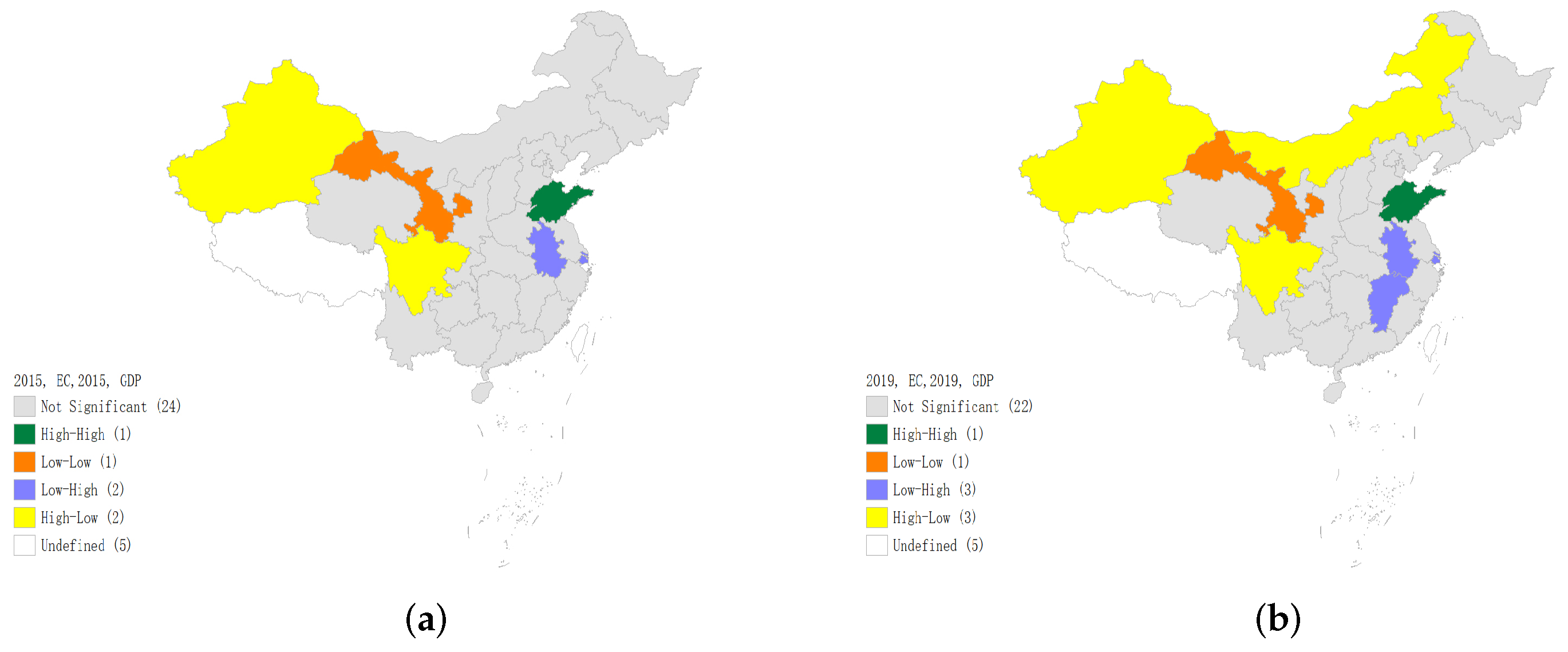
According to the spatial distribution pattern, it is found that energy consumption and GDP in each province of China show specific agglomeration characteristics, respectively. The distribution of the domestic energy consumption presents a spatial distribution pattern of high in the East and low in the West. In addition, the regional distribution of total economic output is also uneven. It is higher in the South and East but lower in the northern and western regions, which indicates unbalanced regional development. In terms of the correlation between energy consumption and GDP, the spatial agglomeration situation of energy consumption and GDP is similar to some extent. Some provinces along the southeast coast of China consistently rank among the top in both energy consumption and GDP, such as Shandong, Zhejiang, Jiangsu, and Guangdong;

(2)

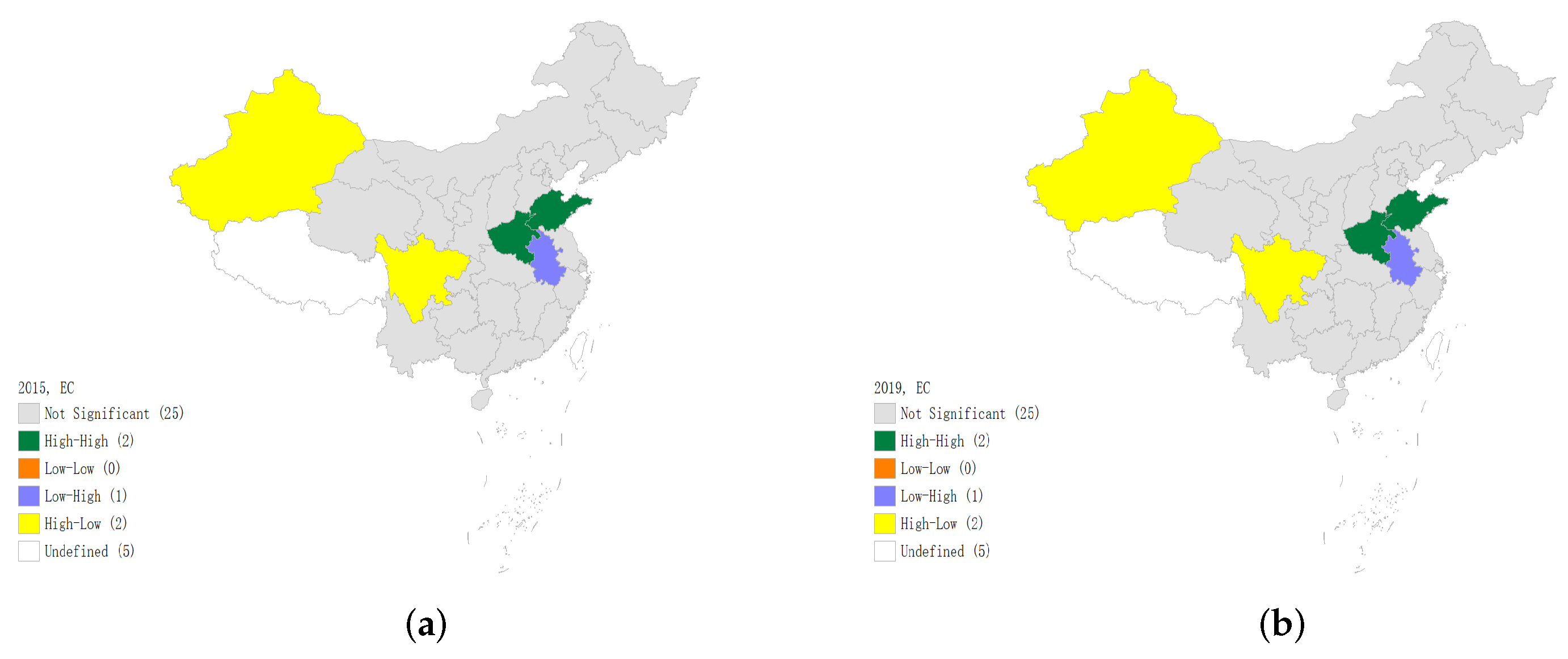
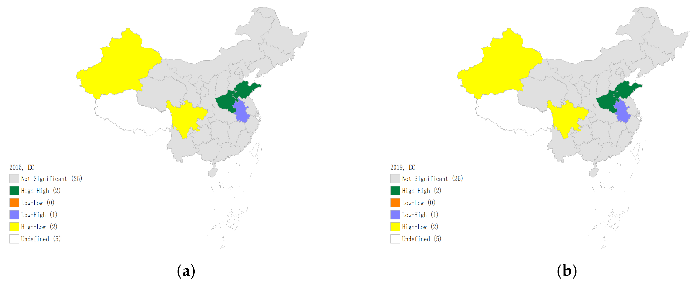
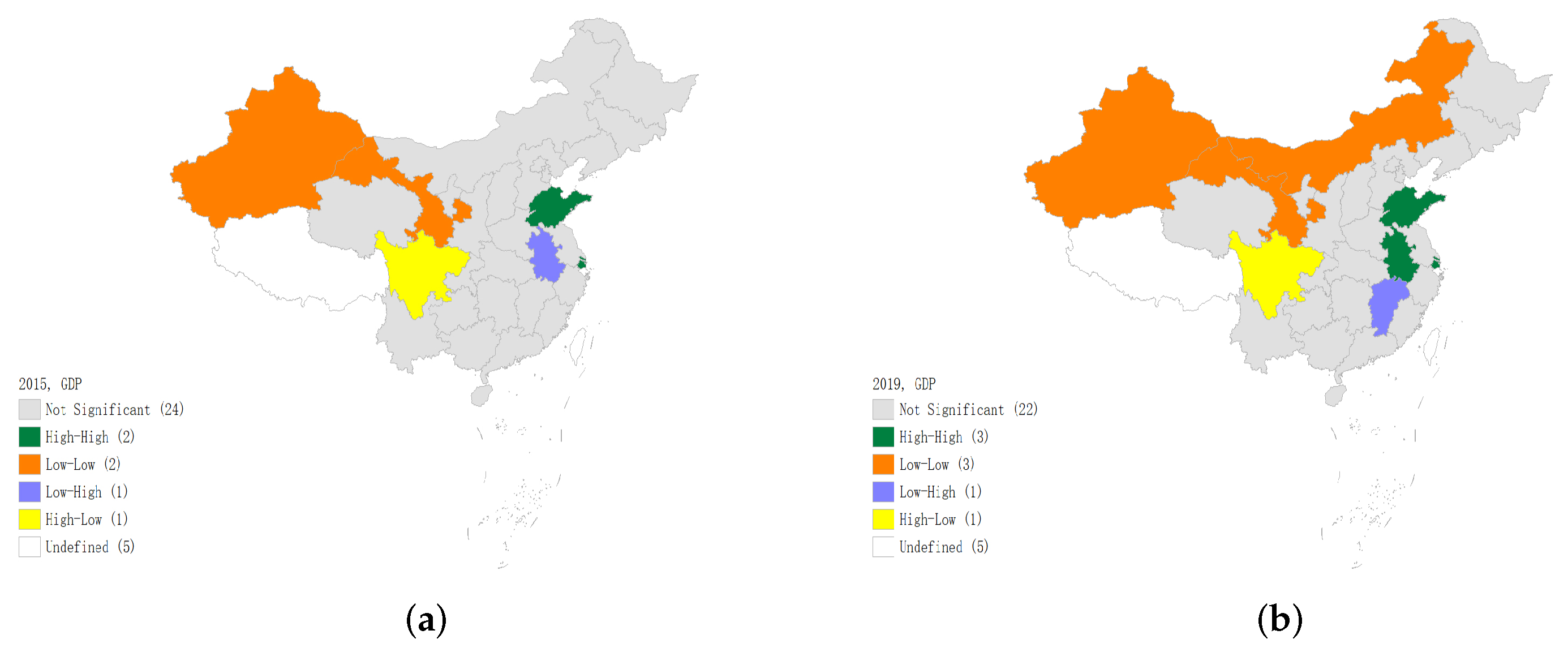
According to spatial correlation test, during the study period, a significant spatial autocorrelation can be witnessed obviously from the aspect of energy consumption and economic development level. Spatial agglomeration has a significant spillover effect, but regional differences in agglomeration types exist. In general, the spatial distribution of energy consumption and economic growth in China shows the agglomeration characteristics of high in the East and South but low in the West and North. Therefore, a particular region with high-value agglomeration forms generally, the core of which is situated in the Yangtze River Delta region and provinces in the middle and lower reaches of the Yangtze River Economic Belt. In the past five years, the spatial agglomeration effect of provinces with similar energy consumption weakened, while provinces with similar GDP levels have increased spatial agglomeration characteristics. As can be seen from the LISA agglomeration map, in terms of economic growth, the agglomeration scope of “high-high” agglomeration regions has been expanded over time. The economic center has been shifting to the central and southeast coastal regions gradually, the economic center has been shifting to the central and southeast coastal regions gradually, a core-periphery model has been formed with the eastern region as the core;

(3)

According to the spatial regression analysis based on partial differential effect decomposition, energy consumption has a significant intraregional spillover effect on economic growth. However, the interregional spillover effects of energy consumption and other control variables differ on economic growth under different spatial weights. A tentative inference from this result is that the relative magnitudes of the “Backwash effect” and “Diffusion effect” differ in different regions. Combined with the Lisa agglomeration map, there is a “high-high” agglomeration in Sichuan and its surrounding areas, indicating a greater “Backwash effect” than the “Diffusion effect” of economic growth in the western region. On the contrary, the “Diffusion effect” of economic development in the eastern region is greater than the “Backwash effect”. In addition, according to the feedback effect, energy consumption could improve regional economic growth by taking a certain region as the center and driving the economic development of the surrounding areas;

(4)

According to the research on different types of energy consumption, the consumption of coal, oil, natural gas, and electricity has a positive spillover effect on economic growth. Among them, oil ranks first in contributing to economic growth, followed by electricity, natural gas, and coal. However, coal consumption accounts for a high proportion of the energy structure, with a low contribution to economic growth. That indicates the possibility of changing China’s extensive economic growth that relies on factor input to high-quality development;

(5)

According to the research on regional heterogeneity, China’s regional economic growth depends on energy consumption, geographical distribution, spatial population density, and urbanization. By relevant policies, 30 provincial units can be divided into three categories for regression tests: eastern and non-eastern, southern and northern, southeast and northwest of “Heihe–Tengchong Line”. It is found that the regions with higher economic development levels are more dependent on energy consumption in the southeast hinterland of China.

This paper systematically explores the energy consumption, economic growth, and the relationship between them of China’s 30 provinces, cities and autonomous regions, combined with spatial and geographical factors on the basis of ordinary panel regression. Actual situations that the direction, path and mode of action of spatial spillover effect may be different due to the individual differences of provincial units. However, the research on the spatial spillover effect of energy consumption on economic growth is based on the assumption that the spillover effects of different provincial units are the same. Therefore, the above issues deserve further exploration and research. Green mountains and clear water are equal to mountains of gold and silver. How to optimize and solve the coordinated development between energy consumption, economic growth, and the environment is an important topic that needs to be continuously studied and explored in the future of the world.

6. Policy Recommendations

Finally, based on the policy background and current development of China, some corresponding policy suggestions are proposed for coping with the two major problems—the regional imbalance between energy consumption and economic level; the constraint of energy consumption on economic growth. The suggestions are as follows:

(1)

Energy consumption and GDP of each province in China show a certain degree of agglomeration, but the interregional development is extremely unbalanced. To address such an imbalance between energy consumption and regional economic levels, the government should make reasonable policy planning for the regional distribution of industrial enterprises. On the one hand, for the “high-high” agglomeration regions (high energy consumption and high economic level), the industrial contributions made by the big energy consumers should be comprehensively analyzed and meticulously considered. They can be encouraged to increase investment in science and technology, develop and utilize clean energy, and establish a market-oriented innovation system for green technologies [59]. The previous concept of adopting an extensive industrial economic development model in the pursuit of short-term economic benefits should be abandoned. Instead, the goal is shifted to establishing and improving a circular economic development system that is green and low-carbon while balancing the growth of the primary, secondary and tertiary industries. On the other hand, for the “low-low” agglomeration regions (low energy consumption and low economic level), reasonable industrial transfers can be implemented based on the Long-Range Objectives to boost the economic growth in the western and northeastern regions of China. In the meantime, the situation of the backwash effect surpassing diffusing effect should be avoided to result in phenomena of “high-low” or “low-high” agglomeration. Chinese government should take clean production, energy conservation, environmental protection, clean energy, and other related sectors as breakthroughs to achieve a reasonable geographical distribution of industries, gradually improve the imbalance issue, and coordinate the development of all provinces [40,60].

(2)

As China’s energy consumption is on the rise, which has significantly contributed to the China’s economic growth, the resulting environmental problems are aggravating. There is still a long way to go towards optimizing the energy structure facing intense energy consumption. Therefore, the government has taken carbon peak and carbon neutrality as long-range goals, adhere to the concept of sustainable development [28,61]. China has witnessed the economic transition from high-speed growth to high-quality development. In this stage, the government should promote green technology innovation, expand the consumption proportion of renewable energy, and accelerate the optimal adjustment of the energy mix. In addition, green and low-carbon development should be integrated into macroeconomic governance. Based on reality, policies should be designated to constantly improve the green trading market mechanism and enhance supervision and oversight. In the field of green finance, appropriate policy support should be provided. All the efforts will be made to ensure the green transformation of work and life and the reasonable resource allocation of energy [62]. Based on the transition and optimization, the upgrading of primary, secondary, and tertiary industries as well as the infrastructure will be driven in a green manner, further adjusting and optimizing our industrial structure. As a result, Chinese government should reduce energy waste and environmental pollution to realize a green, low-carbon, and circular economic development system in which energy use will be more efficient and resource allocation will be more reasonable.

References

1. Ma, Q.; Fu, D. Research on the relationship between energy consumption, technological progress and economic growth. Inq. Econ. Issues 2018, 12, 183–190. [Google Scholar]
2. Xu, G. The Research on the Relationship for Energy Consumption, Corbon Emissions and Economic Growth in China. Ph.D. Thesis, Huazhogn University of Science and Technology, Wuhan, China, 2010. [Google Scholar]
3. Khattak, S.I.; Ahmad, M.; Khan, Z.U.; Khan, A. Exploring the impact of innovation, renewable energy consumption, and income on CO2 emissions: New evidence from the BRICS economies. Environ. Sci. Pollut. Res. 2020, 27, 13866–13881. [Google Scholar] [CrossRef]
4. Dai, S.; Zhang, M.; Huang, W. Decomposing the decoupling of CO2 emission from economic growth in BRICS countries. Nat. Hazards 2016, 84, 1055–1073. [Google Scholar] [CrossRef]
5. Zhuang, R.; Mi, K. Energy consumption, structural changes and air quality:Empirical test based on inter-provincial panel data. Geogr. Res. 2022, 41, 210–228. [Google Scholar]
6. Li, J. Research on the relationship and influence between energy consumption and high-quality economic development in China. Mod. Econ. Res. 2022, 4, 11–20+132. [Google Scholar]
7. De Castro Camioto, F.; Moralles, H.F.; Mariano, E.B.; do Nascimento Rebelatto, D.A. Energy efficiency analysis of G7 and BRICS considering total-factor structure. J. Clean. Prod. 2016, 122, 67–77. [Google Scholar] [CrossRef]
8. Li, J.F.; Gu, A.L.; Ma, Z.Y.; Zhang, C.L.; Sun, Z.Q. Economic development, energy demand, and carbon emission prospects of China’s provinces during the 14th Five-Year Plan period: Application of CMRCGE model. Adv. Clim. Chang. Res. 2019, 10, 165–173. [Google Scholar] [CrossRef]
9. Yu, Q.; Meng, W. The Relationsip between Energy Consumptionand Chinses Economic Growth Based on Panel Data. Syst. Eng. 2008, 26, 68–72. [Google Scholar]
10. Kraft, J.; Kraft, A. On the relationship between energy and GNP. J. Energy Dev. 1978, 3, 401–403. [Google Scholar]
11. Stern, D.I. Energy and economic growth in the USA: A multivariate approach. Energy Econ. 1993, 15, 137–150. [Google Scholar] [CrossRef]
12. Stern, D.I. A multivariate cointegration analysis of the role of energy in the US macroeconomy. Energy Econ. 2000, 22, 267–283. [Google Scholar] [CrossRef] [Green Version]
13. Lee, C.C. Energy consumption and GDP in developing countries: A cointegrated panel analysis. Energy Econ. 2005, 27, 415–427. [Google Scholar] [CrossRef]
14. Mahadevan, R.; Asafu-Adjaye, J. Energy consumption, economic growth and prices: A reassessment using panel VECM for developed and developing countries. Energy Policy 2007, 35, 2481–2490. [Google Scholar] [CrossRef]
15. Tran, B.L.; Chen, C.C.; Tseng, W.C. Causality between energy consumption and economic growth in the presence of GDP threshold effect: Evidence from OECD countries. Energy 2022, 251, 123902. [Google Scholar] [CrossRef]
16. Zhao, J.; Fan, J. Empirical Research on the Inherent Relationship between Economy Growth and Energy Consumption in China. Econ. Res. J. 2007, 42, 31–42. [Google Scholar]
17. Yang, Y.; Chi, Z. Research on the relationship between energy consumption and economic growth in China–Based on error correction model. Res. Econ. Manag. 2009, 612, 39–45. [Google Scholar]
18. Dai, X. Research on the relationship between fossil energy consumption and economic growth in China. Stat. Decis. 2014, 21, 124–126. [Google Scholar]
19. Yan, Q.; Chen, H. Reresearch on the Relationship Between GDP and Energy Consumption. China Popul. Resour. Environ. 2011, 21, 13–19. [Google Scholar]
20. Wang, X. An empirical study on China’s energy consumption and economic growth. Stat. Decis. 2014, 20, 136–138. [Google Scholar]
21. Chen, L.; Yan, L.; Chen, F.; Hu, R. A Study on the Dynamic Relationship between Economic Growth and Energy Consumption. Technol. Innov. Manag. 2020, 41, 75–82. [Google Scholar]
22. Mou, D. A Study of Causal Relations between Energy Consumption and Economic Growth in China. J. Xiamen Univ. Sci. 2008, 2, 100–107. [Google Scholar]
23. Lin, B. Power consumption and China’s economic growth: A study based on production function. J. Manag. World. 2003, 11, 18–27. [Google Scholar]
24. Ma, C.; Chu, H.; Li, K.; Zhou, S. Co-integration Analysis and an Error Correction Model of China’s Energy Consumption and Economy Growth. Syst. Eng. 2004, 22, 47–50. [Google Scholar]
25. Tian, X.; Yang, Z. An empirical study on China’s energy consumption and economic growth. Science 2008, 4, 75–77. [Google Scholar]
26. Zhao, M.; Zhou, D. Structure Relation between Coal Consumption and Economic Growth in China and Its Causality. Prices Mon. 2008, 9, 32–34. [Google Scholar]
27. Xiong, J.; Xu, D. Relationship between energy consumption, economic growth and environmental pollution in China. Environ. Res. 2021, 194, 110718. [Google Scholar] [CrossRef]
28. Wu, Q.; Chen, L.; Zhang, Y.; Cheng, J. Retesting the Granger Causality between Energy Consumption and GDP in China: Based on the Provincial Panel Data Analysis. J. Quant. Econ. 2008, 25, 27–40. [Google Scholar]
29. Li, Q.; Wang, H.; Hu, A. Electricity Consumption and Economic Growth in China–Causality Analysis Based on Provincial Panel Data. China Ind. Econ. 2013, 9, 19–30. [Google Scholar]
30. Liang, J.; Liu, J.; Liu, Z. A nonlinear dynamic study of energy consumption and economic growth. J. Arid. Land Resour. Environ. 2014, 28, 1–6. [Google Scholar]
31. Zhao, X.; li, Y.; Lu, M. Spatial Econometric Analysis of Energy Consumption and Economic Growth in China. Soft Sci. 2012, 26, 33–38. [Google Scholar]
32. Cui, W.; Li, J.; Xu, W.; Güneralp, B. Industrial electricity consumption and economic growth: A spatio-temporal analysis across prefecture-level cities in China from 1999 to 2014. Energy 2021, 222, 119932. [Google Scholar] [CrossRef]
33. Liu, H.; Zhang, Q.; Yang, Q. Urbanization, Spatial Spillover and Regional Economic Growth: China’s Evidence Based on Spatial Regression Model Partial Derivatives Method. J. Agrotech. Econ. 2014, 10, 95–105. [Google Scholar]
34. Ma, X.; Ma, R.; Xu, J. Spatial Structure of Cities and Towns with ESDA-GIS Framework. Acta Geogr. Sin. 2004, 59, 1048–1057. [Google Scholar]
35. Khan, H.; Khan, I.; Binh, T.T. The heterogeneity of renewable energy consumption, carbon emission and financial development in the globe: A panel quantile regression approach. Energy Rep. 2020, 6, 859–867. [Google Scholar] [CrossRef]
36. LeSage, J.; Pace, R.K. Introduction to Spatial Econometrics; Chapman; Hall/CRC: London, UK, 2009. [Google Scholar]
37. Zhang, J.; Wu, G.; Zhang, j. The Estimation of China’s provincial capital stock: 1952–2000. Econ. Res. J. 2004, 10, 35–44. [Google Scholar]
38. Wang, S.; Li, Q.; Fang, C.; Zhou, C. The relationship between economic growth, energy consumption, and CO2 emissions: Empirical evidence from China. Sci. Total. Environ. 2016, 542, 360–371. [Google Scholar] [CrossRef] [PubMed]
39. Xin-gang, Z.; Jin, Z. Industrial restructuring, energy consumption and economic growth: Evidence from China. J. Clean. Prod. 2022, 335, 130242. [Google Scholar] [CrossRef]
40. Dong, T.; Deng, S. Diversification of Energy Consumption Structure and Regional Haze Pollution: Empirical Research on Yangtze River Economic Belt. Consum. Econ. 2019, 35, 64–76. [Google Scholar]
41. Li, X.; Ran, G. How does the development of digital finance affect the quality of technological innovation? Mod. Econ. Res. 2021, 9, 69–77. [Google Scholar]
42. Du, K.; Lin, B. Understanding the rapid growth of China’s energy consumption: A comprehensive decomposition framework. Energy 2015, 90, 570–577. [Google Scholar] [CrossRef]
43. Salim, R.; Yao, Y.; Chen, G.; Zhang, L. Can foreign direct investment harness energy consumption in China? A time series investigation. Energy Econ. 2017, 66, 43–53. [Google Scholar] [CrossRef]
44. Jalil, A.; Feridun, M. Energy-driven economic growth: Energy consumptio–Economic growth nexus revisited for China. Emerg. Mark. Financ. Trade 2014, 50, 159–168. [Google Scholar]
45. Liddle, B.; Lung, S. Revisiting energy consumption and GDP causality: Importance of a priori hypothesis testing, disaggregated data, and heterogeneous panels. Appl. Energy 2015, 142, 44–55. [Google Scholar] [CrossRef]
46. Ahmad, A.; Zhao, Y.; Shahbaz, M.; Bano, S.; Zhang, Z.; Wang, S.; Liu, Y. Carbon emissions, energy consumption and economic growth: An aggregate and disaggregate analysis of the Indian economy. Energy Policy 2016, 96, 131–143. [Google Scholar] [CrossRef]
47. Dong, L.; Liang, H. Spatial analysis on China’s regional air pollutants and CO2 emissions: Emission pattern and regional disparity. Atmos. Environ. 2014, 92, 280–291. [Google Scholar] [CrossRef]
48. Oliveira, C.; Antunes, C.H. A multiple objective model to deal with economy–energy–environment interactions. Eur. J. Oper. Res. 2004, 153, 370–385. [Google Scholar] [CrossRef]
49. Li, J.; Liu, Y. Data Processing in Regional Energy, Economy and Environment System Development Theories Research. In Advanced Materials Research; Trans Tech Publications Ltd.: Zurich, Switzerlandm, 2014; Volume 1046, pp. 550–553. [Google Scholar]
50. Liu, H.; Yang, Q. Financial Deepening, Spatial Spillover and Economic Growth: China’s Evidence Based on Spatial Regression Model Partial Derivatives Method. Financ. Econ. Res. 2014, 29, 86–95. [Google Scholar]
51. Ying, L.G. Understanding China’s recent growth experience: A spatial econometric perspective. Ann. Reg. Sci. 2003, 37, 613–628. [Google Scholar] [CrossRef]
52. Jiang, L.; Ji, M.; Bai, L. Characterizing China’s energy consumption with selective economic factors and energy-resource endowment: A spatial econometric approach. Front. Earth Sci. 2015, 9, 355–368. [Google Scholar] [CrossRef]
53. Xie, H.; Liu, G.; Liu, Q.; Wang, P. Analysis of spatial disparities and driving factors of energy consumption change in China based on spatial statistics. Sustainability 2014, 6, 2264–2280. [Google Scholar] [CrossRef] [Green Version]
54. Wang, J.; Ning, Y. Research on Relationship among Energy Consumption, Coal Consumption and Economic Growth. J. Tech. Econ. Manag. 2011, 12, 9–12. [Google Scholar]
55. Hu, Y.; Zhang, X.; Li, J. Export, Geography Conditions and Air Pollution. China Ind. Econ. 2019, 9, 98–116. [Google Scholar]
56. Brun, J.F.; Combes, J.L.; Renard, M.F. Are there spillover effects between coastal and noncoastal regions in China? China Econ. Rev. 2002, 13, 161–169. [Google Scholar] [CrossRef] [Green Version]
57. Li, S.; Lu, J.; Yan, J.; Liu, X.; Kong, F.; Wang, J. Spatiotemporal variability of temperature in northern and southern Qinling Mountains and its influence on climatic boundary. Acta Geogr. Sin. 2018, 73, 13–24. [Google Scholar]
58. Kong, X.; Fu, M.; Zhao, X.; Wang, J.; Jiang, P. Ecological effects of land-use change on two sides of the Hu Huanyong Line in China. Land Use Policy 2022, 113, 105895. [Google Scholar] [CrossRef]
59. Liu, K.; Lin, B. Research on influencing factors of environmental pollution in China: A spatial econometric analysis. J. Clean. Prod. 2019, 206, 356–364. [Google Scholar] [CrossRef]
60. Xu, X.; Yang, G.; Tan, Y.; Zhuang, Q.; Tang, X.; Zhao, K.; Wang, S. Factors influencing industrial carbon emissions and strategies for carbon mitigation in the Yangtze River Delta of China. J. Clean. Prod. 2017, 142, 3607–3616. [Google Scholar] [CrossRef]
61. Guo, J.; Xu, Y.; Pu, Z. Urbanization and its effects on industrial pollutant emissions: An empirical study of a chinese case with the spatial panel model. Sustainability 2016, 8, 812. [Google Scholar] [CrossRef] [Green Version]
62. Zhang, Q.; Yang, J.; Sun, Z.; Wu, F. Analyzing the impact factors of energy-related CO2 emissions in China: What can spatial panel regressions tell us? J. Clean. Prod. 2017, 161, 1085–1093. [Google Scholar] [CrossRef]
Figure 1. Spatial pattern of China’s regional energy consumption in 2015 (a) and 2019 (b).
Sustainability 14 09563 g001
Figure 2. Spatial pattern of China’s regional economic growth in 2015 (a) and 2019 (b). Figure 1 and Figure 2, drawn by the software GeoDa, are spatial quantile map of quartiles, that is, the values of all sample variables in a specified time range are arranged in ascending order and divided into four intervals of the same length, which are correspondingly represented by four colors from light to dark in the map, to show the distribution of research object visually. The legend in the bottom left corner of the picture shows the correspondence between the color block and the number range.
Sustainability 14 09563 g002
Figure 3. LISA agglomeration map of the China’s regional energy consumption in 2015 (a) and 2019 (b).
Sustainability 14 09563 g003
Figure 4. LISA agglomeration map of China’s regional economic growth in 2015 (a) and 2019 (b).
Sustainability 14 09563 g004
Figure 5. Bivariate LISA agglomeration map of China’s regional energy consumption and economic growth in 2015 (a) and 2019 (b).
Sustainability 14 09563 g005