1. Introduction
The economic growth of a country is closely related to its electrical energy consumption as depicted in
Figure 1, where the relationship between the Gross Domestic Product (GDP) compared to the energy consumption of the countries belonging to the Organization for Economic Cooperation and Development is clearly visible. There is a clear correlation between these two variables [
1]. However, this relationship is not always maintained when GDP decreases because, during a slowdown in the economy, power plants need to remain operational and this situation prevents electricity consumption from decreasing at the same rate as economic activity slows down.
The constant use of electricity is one of the main methods for economic development. A regular problem is the poor power quality in the supply network; this issue implies a large economic investment from the supplier side due to the need of high efficiency equipment, expensive devices for transitory events suppression inside the load center and through the general electricity system. It also causes an important economical investment from the user who is forced to hire highly qualified personnel to measure, identify, and provide an optimal solution to correct the potential problems that may arise due to a poor quality of electrical power. Electric power consumers are usually classified under three categories defined as residential, commercial and industrial. Additionally, the consumed power in any of the three categories mentioned above will vary according to electrical load type connected; the highly inductive loads as well as the nonlinear loads are the most important, as they are closely related to harmonic events in voltage and current as well as high losses in the efficiency and poor quality of electrical energy [
2].
One of the fundamental parameters to assess the quality of power in a load center along with harmonic content is the power factor (PF); this parameter indicates the efficiency in the use of supplied electrical power from the grid to the facility. Ideally, the PF should be equal to 1 and any deviation from this value implies loss of electrical power. The expression for calculating the PF is shown in Equation (1) describing the dependence of this parameter on the active power and the apparent power [
3].
Having a low PF value [
4,
5] can cause numerous disadvantages like bigger sizing in industrial equipment, additional voltage regulators and larger conductor wiring to withstand higher currents to name a few. A low PF value therefore represents a higher economical cost for the user as much as for the supplier because it implies that consumed power from grid is very inefficiently converted in useful work (energy wastage). A low PF usually could have two different origins namely high harmonic content in current waveform or phase voltage-current shift, being by far the latest the most common. Therefore, in order to improve a low PF value, a power factor compensation (PFC) system is usually applied [
6,
7,
8] consisting of an electrical circuit that supplies reactive power to the grid. Because of the voltage-current phase shift is caused by high inductive loads, a capacitor bank or power electronics converters (STATCOMs) are usually utilized to compensate and improve the PF. Operation of these PFC is based on the connection/disconnection of the PFC from the grid depending on real-time measurements of phase current and voltages waveforms. As a consequence, this implies an increased complexity and cost for the PFC system due to the need for a full sensor network required to monitor the phase currents, voltages, and powers. Indeed, in order to detect and eventually improve low PF values, it will be usually necessary to request at the supplier company the installation of smartmeters [
9], which are devices capable of measuring and recording in real time the key parameters of electrical consumption as phase voltages and currents, consumed active and apparent power, power factor, harmonics content (THD), etc. From the consumer side, it can be necessary to use power quality analyzers for monitoring and recording in real time the PF [
10] implying high economical costs.
Nevertheless, usually PF variations show a cyclical behavior as they are related to activation/deactivation of the inductive or non-linear loads. Thus, if these cyclic variations could be predicted on a daily, basis it could be very appealing, as no sensor network would be required for PF compensation and the number of recorded electrical variables it could be minimized. This minimization would simplify the monitoring procedure and reduce the investment cost for the consumer. Evidently, this alternative implemented by the consumer can prevent and correct present and potential failures in the electrical installation that also has important costs for the supplier.
The artificial intelligence (AI) could provide a valid option to solve issues concerning power quality and in particular about PF because in the past few years it has been widely documented its influence in multiple domains such as image processing [
11], power electronics [
12], medical [
13], and many other domains.
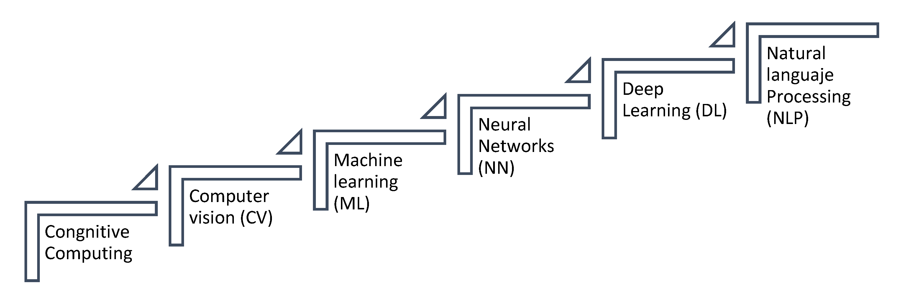
Artificial intelligence can be classified into different disciplines as Computer Vision (CV), Machine Learning (ML), Neural Networks (NN), Deep Learning (DL) and Natural Language Processing (NLP) as depicted in
Figure 2.
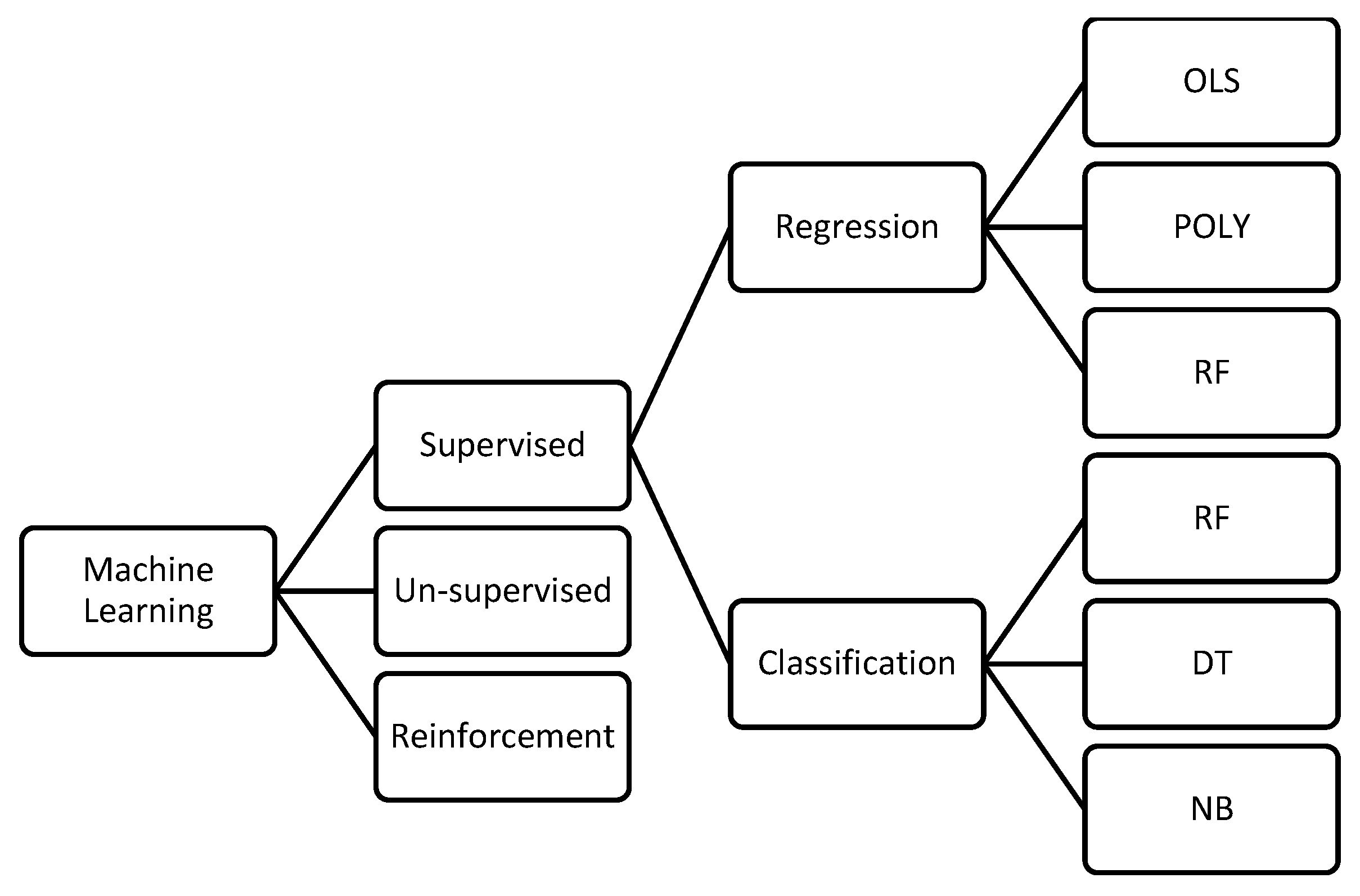
In
Figure 3, a classification for machine learning domain is shown accordingly to the learning process—namely, supervised, unsupervised, and reinforcement learning.
Due to the nature of our data, which is tabular type, we decided to use a supervised ML technique. Moreover, supervised ML techniques have two options; the first are regression methods and the second classification methods. The use of one of them depends on the nature of the analyzed data. In our case, power factor data are continuous type therefore it is recommended to use the regression methods, which in turn is divided into different algorithms being OLS, Poly and RF the most important. Below, a brief description of each algorithm is provided
Decision Trees (RF) are used for both regression and classification problems. They visually flow like trees, hence the name, and in the regression case, they start with the root of the tree and follow splits based on variable outcomes until a leaf node is reached and the result is given. Random Forest algorithm combines ensemble learning methods with the decision tree framework to create multiple randomly drawn decision trees from the data, averaging the results to output a new result that often leads to strong predictions/classifications.
Ordinary Least Squares regression (OLS) is a common technique for estimating coefficients of linear regression equations which describe the relationship between one or more independent quantitative variables and a dependent variable (simple or multiple linear regression).
Polynomial Regression (Poly) is a form of regression analysis in which the relationship between the independent variables and dependent variables are modeled in the nth degree polynomial. Polynomial Regression models are usually fit with the method of least squares. This algorithm is a special case of Linear Regression where we fit the polynomial equation on the data with a curvilinear relationship between the dependent and independent variables.
In particular, AI in electrical power systems has been used in several areas such event detection as flickers and surge voltage transients [
14], frequency regulation, distribution system control [
15], power factor correction [
8], voltage sag and swell problems [
16], and power quality disturbances detection and classification [
17].
In this work, a model for PF prediction using only phase currents (no phase voltages measurements required) is proposed. This solution provides a reliable prediction of PF fluctuations by using (ML) techniques, in particular linear regression models have been used. The results obtained from model deployment are very promising although for PF variations predictions in installations where renewable energy systems are operating it should be further optimized.
2. Materials and Methods
For this work, four electric load centers (ELC) were selected (listed in
Table 1) based on the requirement for electrical local regulations for each site specified by Mexico’s network code [
18]. All ELCs analyzed have the same business division (gas stations); therefore, the type of electrical equipment is more or less similar between them. However, there are other important differences among these sites such frequency of service, contracted load, neighboring electrical installations, brands and characteristics of the installed equipment, years of service, maintenance scheme, geographical site, and infrastructure of the supplier company as well as installed load.
Obtaining data from the selected centers (ELC) was performed with a MYeBox 1500
® three phase power quality analyzer from Circutor
®. Data is stored in a 25 GB external SD memory card. Each selected ELC was monitored for a 7-day time period by using demand period storage rate of 5 min and recording current measurements for each phase along with real-time PF calculations [
19].
Figure 4 shows the connection diagram of the analyzer in a 3F + N system [
20].
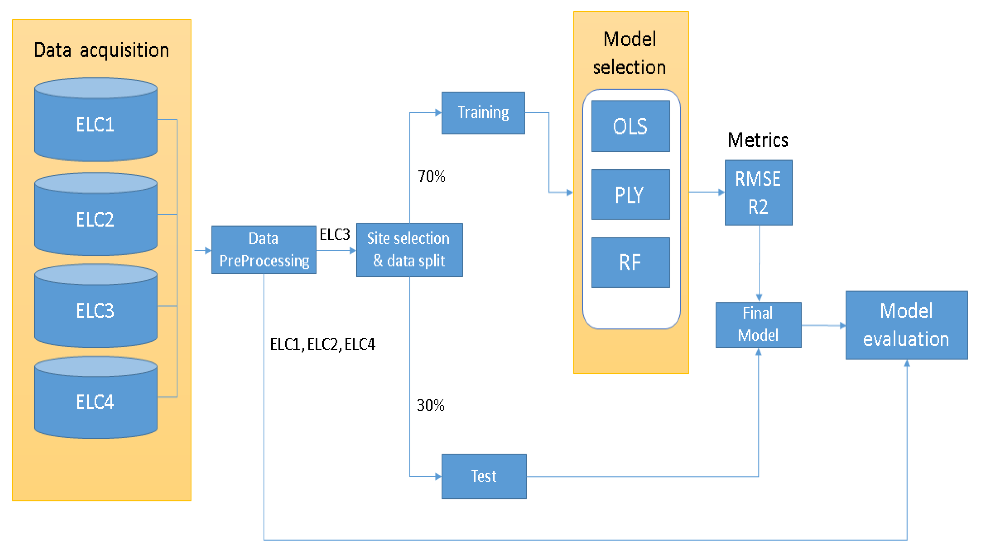
Once the data for each site was acquired, the procedure for ML analysis could be performed. Procedure for ML model building, testing and evaluating is graphically depicted in
Figure 5 and is the typical used in the literature [
21]. First, datasets are preprocessed (cleaning and tabular formatting), secondly site selection is performed based on statistical results and data splitting for model training using 70% of data for training and 30% of data for testing. Next, several linear regression algorithms are used for training and the statistical results are used to evaluate their performance. Finally, the model is tested in other selected sites, and statistical results are analyzed for final model evaluation.
3. Results and Discussion
All data processing and display as well as ML model training and test were performed with Python environment [
22]. As described above in
Section 2, a total of 4 sites belonging to gas stations business category were analyzed.
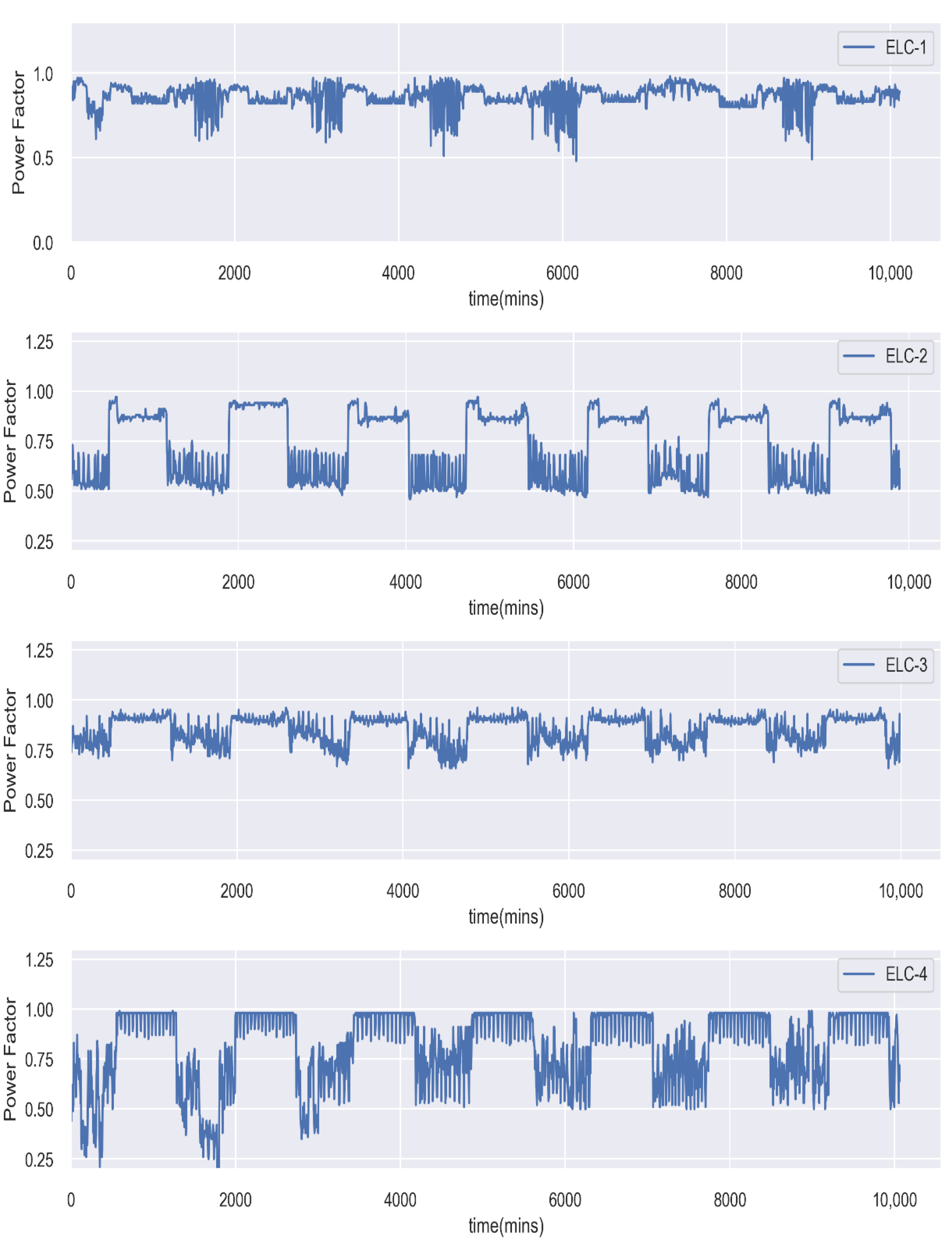
Figure 6 shows monitored PF data plotted as a function of measurement time.
Figure 6 depicts the behavior of PF for a defined period of time (10,000 min i.e., 7 days). As it can be observed, each site shows cyclic variations of PF, but they are different between them because the equipment connected to the electrical grid in each site has different specifications. The cyclic variation of PF can be related to highly inductive loads operating at certain daily hours. For example, for site ELC-2 it can be seen that PF diminishes down to 0.5 between 8:00 p.m. and 8:00 a.m. corresponding to the night-shift when big equipment (high inductive loads) is operated.
The purpose of any supervised ML model is to establish a function of the predictors; that best explains the response variable (target). In this case, the predictors are the phase currents and the target variable will be the power factor value as depicted in
Table 2.
For this function to be stable and to be a good and reliable estimate of the target variable, it is very important that these predictors are correlated with it. Therefore, the first step would be to perform a correlation analysis between these variables. The correlation is a statistical measure that indicates the extent to which two or more variables move together. A positive correlation indicates that the variables increase or decrease together. A negative correlation indicates that if one variable increases, the other decreases, and vice versa. The correlation coefficient (r) indicates the strength of the linear relationship that might be existing between two variables. A correlation map involving the phase voltages, currents and power factor for every location was performed, and the results are shown in
Figure 7. It can be observed that the highest correlation was obtained between phase currents and power factor whereas a weak correlation factor is observed between phase voltages and PF. Therefore, the use of only phase currents to predict PF is justified.
Once the correlation has been stablished for all sites, it is necessary to carefully select the site that will be used for ML model training. At first glance, site ELC-3 seems appealing for selection as is the one showing the higher correlation factors between phase currents (IL1, IL2, IL3) and PF being 0.8, 0.8, and 0.85, respectively.
However, this decision should be validated by exploring in detail the characteristics of the dataset. Specifically, the good performance of any ML model relies upon data distribution and for linear regression models four main characteristics should be taken into account: additivity and linearity of effects, constant error variance, normality of errors and zero correlation between errors. Therefore, for ML applications it is always preferable to have a normal (gaussian) distribution as described by Equation (2):
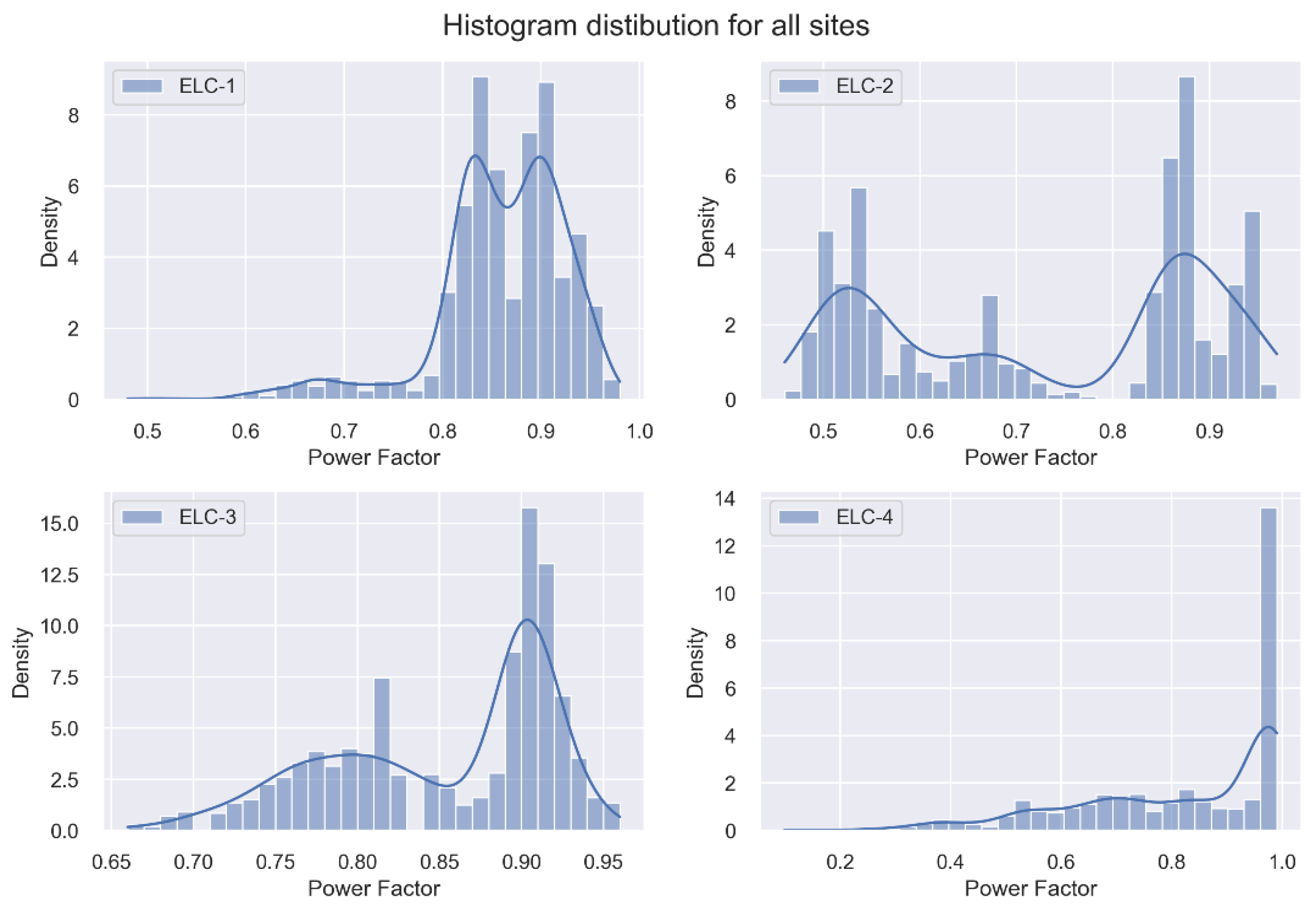
However, it is not mandatory that data should always follow normality. As a matter of fact, some ML models work very well in the case of non-normally distributed data like decision tree models which don’t assume any normality and work fairly well. In order to analyze data distribution for each site histograms and Kernel Distribution Estimation (KDE) plots are very useful. Histogram plots give an estimate of the probability distribution of a continuous variable whereas KDE plots depict the probability density function of the continuous or non-parametric data variables.
Figure 8 displays the histograms and KDE plots for the 4 sites showing that for ELC-1, ELC-2, and ELC-4 a broad data dispersion along with multimodal-type distribution is observed. Conversely, for ELC-3 site a bimodal-type distribution and a slightly narrower data dispersion was detected thus becoming a more suitable option for ML model training.
Following and to confirm that ELC-3 site is the most suitable for model training a test-train split for each dataset was performed using sizes adjusted at 70% for training and 30% for testing, setting random_state = 101.
The Mean Squared Error, Mean absolute error, Root Mean Squared Error, and R-Squared or Coefficient of determination metrics are the evaluation metrics used in regression analysis.
The Mean absolute error (
MAE) represents the average of the absolute difference between the actual and predicted values in the dataset. This parameter is calculated with Equation (3):
Mean Squared Error (
MSE) represents the average of the squared difference between the original and predicted values in the data set. This parameter is calculated with Equation (4):
Root Mean Squared Error is the square root of Mean Squared error. This parameter is calculated with Equation (5):
MSE and RMSE penalizes the large prediction errors vi-a-vis MAE. However, RMSE is widely used than MSE to evaluate the performance of the regression model with other random models, as it has the same units as the dependent variable (Y-axis).
The coefficient of determination or
R-squared represents the proportion of the variance in the dependent variable which is explained by the linear regression model. This parameter is calculated with Equation (6):
The lower value of MAE, MSE, and RMSE implies higher accuracy of a regression model. However, a higher value of R2 is considered desirable.
An ordinary least square regression (OLS) algorithm was algorithm was used and the evaluation metrics as
MAE,
MSE,
RMSE and
R2 were calculated for each site. As observed from results depicted in
Table 3, ELC-3 site showed the lowest
RMSE as well as the higher
R2 value.
Once the site for model training was confirmed, the next step was to compare the statistical parameters with the three main linear regression ML models, specifically ordinary least square regression (OLS), polynomial regression (Poly), and random forest regression (RF). The hyperparameters configuration setting for Poly regression was (degree = 2) whereas for RF algorithm setting was (n_estimators = 100, random_state = 101, criterion = “absolute_error”, max_depth = 19).
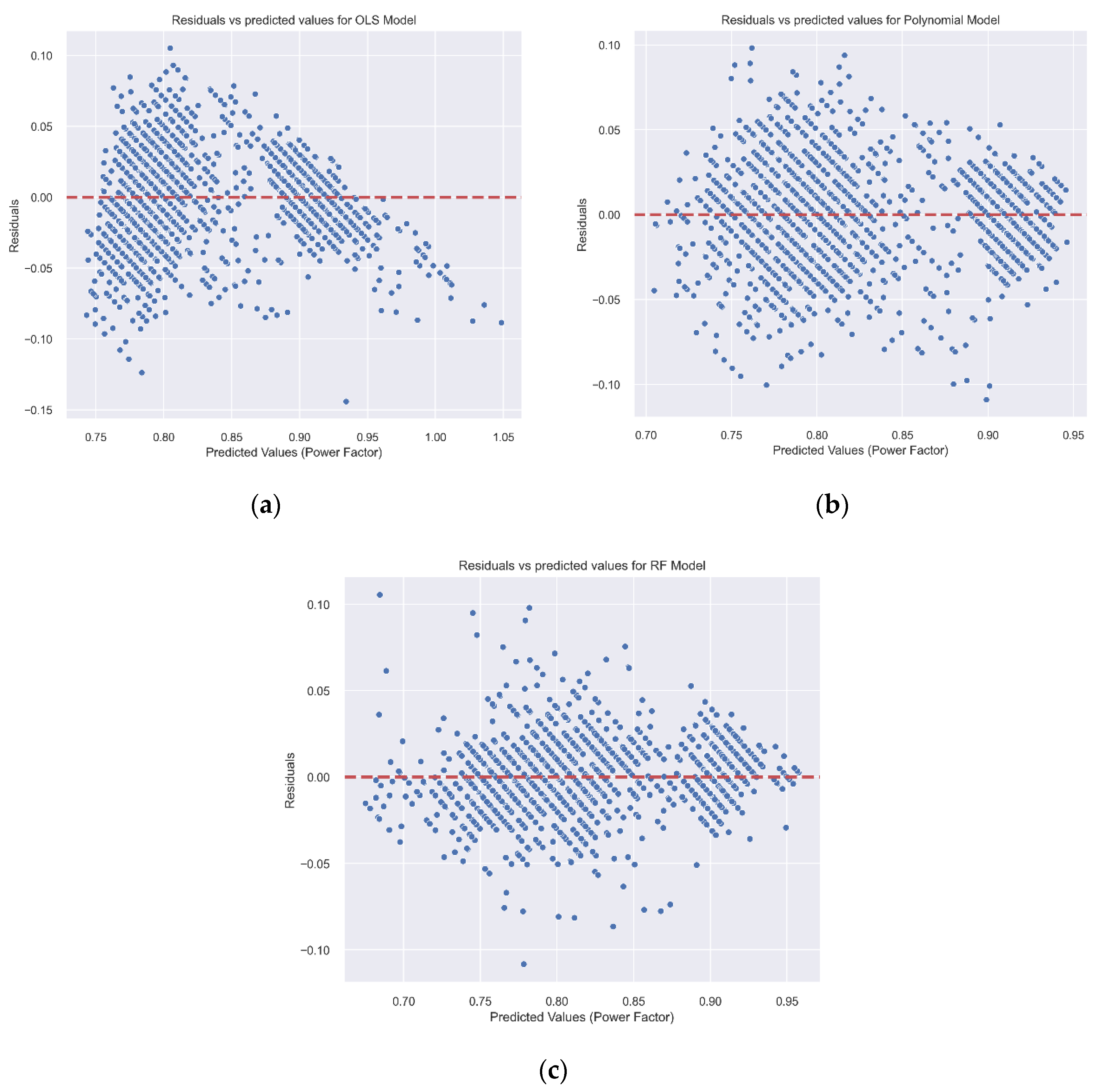
In
Figure 9, an error residuals (calculated errors between observed and predicted values) plot is depicted. In this type of plot, a random distribution of error residuals should be observed in order to consider linear regression as suitable technique for prediction. Consequently, the results obtained from
Figure 9 confirm that for all three models the random behavior in the residuals distribution is present. Furthermore, it can be observed that RF model has the most compact residuals distribution (fewer spread) implying that calculated errors between observed and predicted values are lower than the other two models (OLS and polynomial).
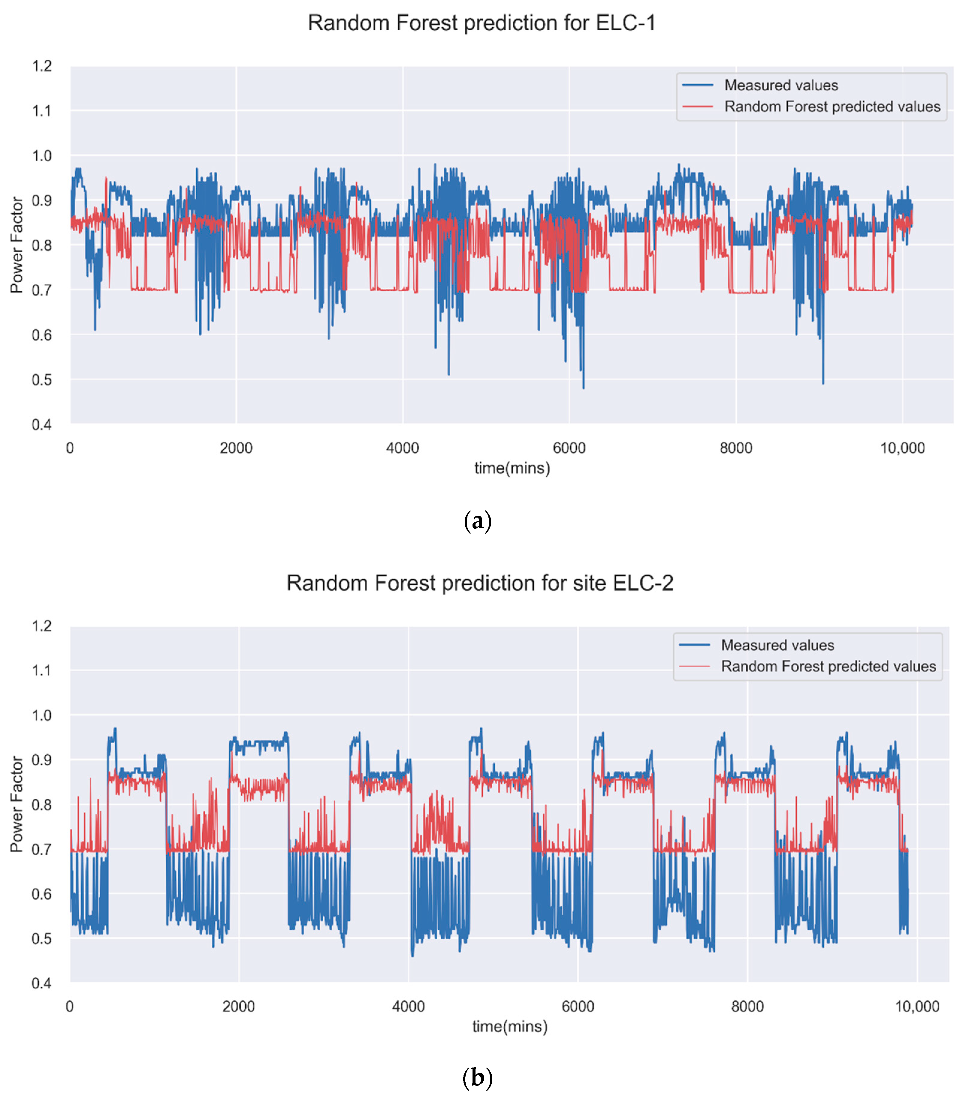
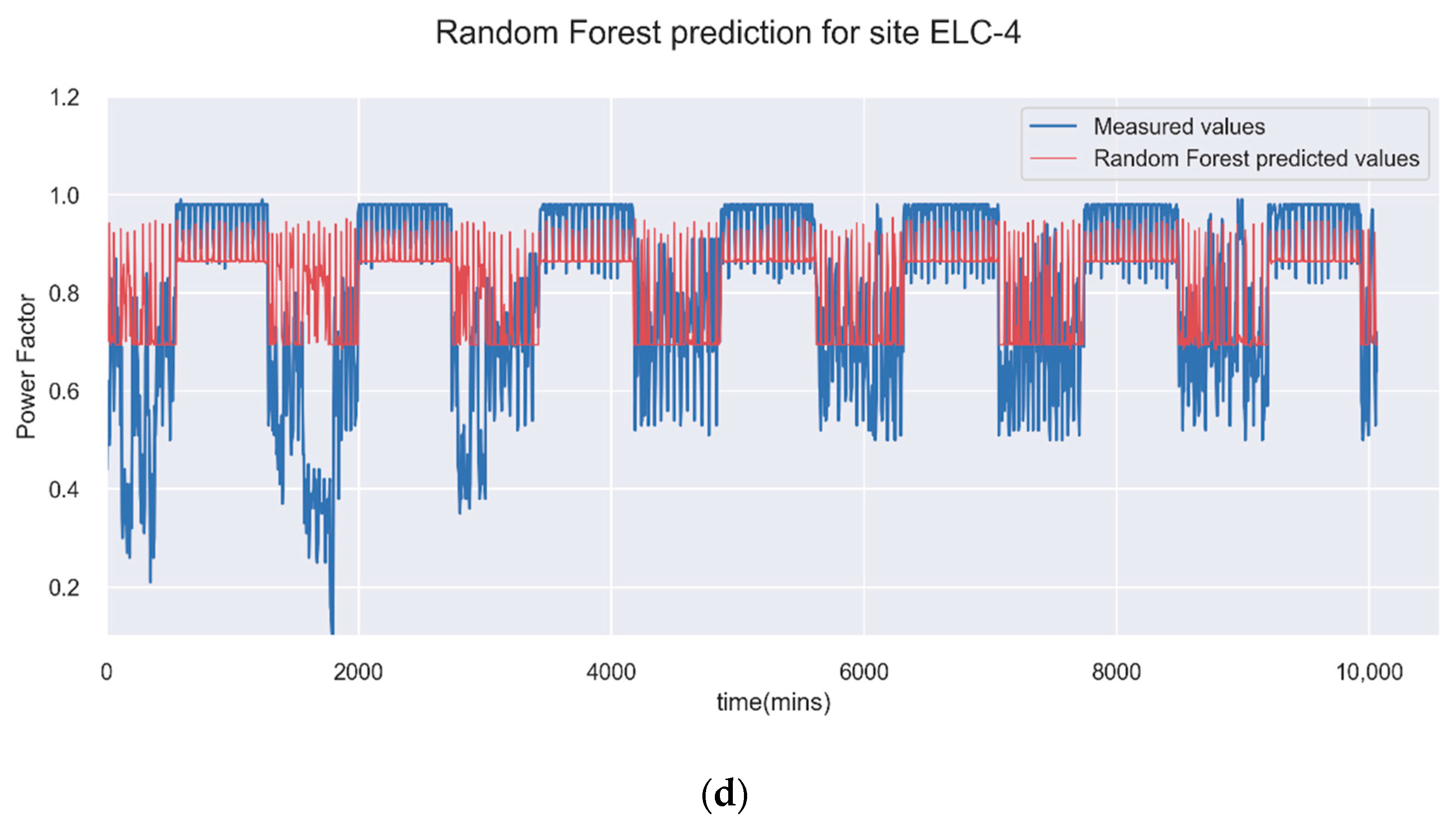
Finally, last step was to predict the PF variations for the remaining three sites (ELC-1, ELC-2, and ELC-4) using the previously trained and adjusted RF model.
Figure 10 shows the fitting results for each of these locations while
Table 3 displays the statistical parameters for each site.
The plots in
Figure 10 show a rather good fit between model predicted data and actual measured PF values. These results validate the satisfactory performance of the proposed model where only phase currents were taken into account. Moreover, as observed from
Table 4, most of the sites show a fairly high R
2 coefficient (0.85) along with a low RMSE error except for ELC-4 where RMSE error is slightly bigger (0.175). The higher discrepancy obtained for site ELC-4 could be associated to a weaker correlation observed between phase currents and PF for this particular site (see
Figure 7). Therefore, a different approach should be considered like taking into account also the phase voltages or consider only one phase current (i.e., IL3) for model prediction.

