Intermediate Effect of the COVID-19 Pandemic on Prices of Housing near Light Rail Transit: A Case Study of the Portland Metropolitan Area

Abstract

This study explored the dynamics of a residential property value premium for proximity to a light rail transit (LRT) station in the intermediate term (roughly two years) since the pandemic. We applied a longitudinal quasi-experimental design using repeat sales data from the Portland Metropolitan Area, Oregon. Our results indicate that the effect of the pandemic on prices of housing near LRT stations differs between single-family and multi-family markets. Since the pandemic outbreak, there has been no statically significant difference in the price appreciation between single-family (SF) housing within an LRT service area and otherwise similar SF homes; however, for multi-family (MF) homes, those within an LRT service area have experienced a 3.0% lower price appreciation rate than MFs outside such areas with similar characteristics. Our findings help better highlight the impact of the pandemic on the real estate market and can inform discussions about longer-term changes in post-COVID cities and their planning.

1. Introduction

The COVID-19 pandemic has been reported to have shifted how people travel and where they prefer to live [1,2]. At the peak of the pandemic, there was a sharp decline in overall travel. As lockdown policies began to ease, travel started to slowly resume, with transit ridership being the slowest to recover. Additionally, many scholars and journalists postulate that the crisis will transform our relationship with location, as people adjust their work and daily lives [3]. For instance, since the pandemic, the preference has shifted toward suburban and exurban areas from denser urban areas such as central business districts [4]. These changes raise the question of whether the COVID-led disruptions have been reflected in the real estate market, especially for homes proximate to light rail transit (LRT) stations, which typically enjoy a price premium compared to otherwise similar homes.

Therefore, we attempted to answer how the residential property (i.e., single-family and multi-family housing) price premium for proximity to LRT stations was affected by the COVID-19 pandemic in the intermediate term (roughly two years). We applied a longitudinal quasi-experimental design using repeat sales data with a case study of the Portland Metropolitan Area, Oregon, which allowed us to quantify the effects of the pandemic on single-family and multi-family home markets. While it is premature to assess the long-term impacts of COVID-19 on the real estate market, as its effects are still unfolding, this paper contributes by (1) providing a timely snapshot of the effects of the COVID-19 pandemic on the housing market in the intermediate term in the Portland Metropolitan Area and (2) helping inform discussions about changes in the post-COVID cities and their planning.

The remainder of this paper is structured as follows. Section 2 summarizes and synthesizes the previous literature. Section 3 presents the research design, including the methodological approaches and data used in this research. Section 4 presents the findings. Finally, Section 5 and Section 6 discuss the results and conclude this study.

2. Literature Review

We begin with a literature review of two topics: (1) an overview of the property value premium resulting from the proximity to public transit facilities, particularly regarding light rail transit (LRT) stations in the U.S. context; (2) the impacts of COVID-19 on transit use and the real estate market. We then synthesize the theoretical frameworks and findings and present the research gaps and our research questions.

2.1. Property Value Premium

There is some debate about whether a city should build a transit system when considering its costs and benefits, although transit systems have the potential to generate positive economic, social, and environmental externalities [5,6]. On the one hand, it is essential to develop and improve public transportation systems to form sustainable urban environments, since these modes of transportation can contribute to an increased willingness to pay in exchange for improved accessibility for citizens, particularly marginalized population groups [7]. On the other hand, the resulting transit-induced capitalization into property values has made many scholars express their concerns; for instance, vulnerable people may be forced to move out or live in substandard housing in areas with better transit accessibility [8]. To achieve sustainable urban development, it is essential to gain a deep understanding of the land value capture mechanism in relation to the accessibility of public transportation. This understanding can serve as the foundation for developing strategies to address the detrimental effects associated with the value premium while still delivering the benefits, which, in turn, helps in attaining a sustainable urban environment.

Accordingly, the well-known adage in the real estate industry is “location, location, location”. This implies that location advantages such as good transit accessibility can impact on property values positively [9], known as a property value premium (also known as value uplift). In addition, economic theories have established the well-known downward-sloping bid–rent curve that demonstrates the trade-off between transportation costs and land values, whereby lower transportation costs in accessible locations result in higher land values [10,11,12,13].

Furthermore, the ample empirical literature has generally confirmed the association between the transit infrastructure proximity and the values of the surrounding properties [14,15,16]. More specifically, regarding the LRT proximity effect in the U.S. context, Cervero and Duncan [17] found the capitalized benefits to be associated with proximity benefits in residential properties. Additionally, Hess and Almeida [18] observed the association between proximity to an LRT station and residential property value premiums in Buffalo, New York. Overall, the range of elasticity is been between −0.01 and −0.10, although the elasticity can vary depending on many factors, such as the study area and methodological approaches. The meta-analysis performed by Hamidi et al. [19] found the premium rates for distances of 0 to 0.25 miles (5.40) and 0.25 to 0.5 miles (5.86) when using discrete distance bands.

Beyond the static effect with a single equilibrium, another body of empirical studies has identified a causal relationship, whereby transit accessibility can increase property values [20,21,22]. For example, Kim and Lahr [23] analyzed the impact of the Hudson–Bergen Light Rail on residential property values in New Jersey and confirmed that transit proximity led to a value uplift.

Moreover, the previous literature started to examine the effect of transit from a temporal dynamic perspective [16,24,25,26]. For instance, Knaap et al. [27] found that the announcement of plans for the LRT system in Washington County, Oregon, triggered a premium. The announcement of the transportation projects generated a net positive premium, which can be translated into an anticipated capitalization effect [28,29]. Golub et al. [30] also found that the prices of properties significantly and differently responded to the five planning phases of the LRT system in Phoenix, Arizona.

Interestingly, previous studies have suggested a “faded-out” property value premium when transit systems start to operate [31]. Yan et al. [32] revealed that while proximity to an LRT station in Charlotte, North Carolina, had a significant and negative impact on home prices before the operation, the effects became insignificant during the operation phase. An analysis by Cao and Lou [24] indicated that a premium for single-family housing existed after the announcement of the LRT system in Minneapolis but not before its operation. Ke and Gkritza [33] found that while the property value increased after the announcement of the LRT project, the premium reduced or disappeared in size after the LRT began operating.

In summary, a body of empirical studies has suggested that a premium for proximity to LRT exists, and that the premium can vary over time and even dissipate.

2.2. Impacts of COVID-19 Pandemic

2.2.1. Transit Ridership

The pandemic’s drastic impact on transit usage is well-known. Due to lockdowns, business closure, shifting to working from home, and travel restrictions, such as “stay-at-home” orders, as well as the potential risk of spreading COVID-19 among passengers [2], transit ridership crashed [34,35,36]. For example, in the U.S., the Washington Metropolitan Area Transit Authority [37] reported that Metrorail ridership decreased by 90% at the end of March 2020. Likewise, Hu and Chen [36] found that the COVID-19 pandemic resulted in an average 72.4% decline in transit ridership in Chicago, Illinois. Nonetheless, Jung [38] found that transit ridership in low-income groups remained unchanged during the COVID period.

2.2.2. Real Estate Market

Several studies have explored the changes in residential location preferences due to the COVID-19 pandemic. For instance, Nanda et al. [4] highlighted that despite the advantages of central business districts, such as better access to amenities and employment opportunities, the housing location preference shifted toward secluded housing in the suburbs immediately after the pandemic outbreak. Similarly, Ramani and Bloom [39] found that since March 2020, the average rental and housing prices in the largest U.S. metropolitan areas had declined or remained flat in the central business districts and the highly-populated areas, while prices increased in areas with lower population density. In addition, Liu and Su [40] examined aggregate housing price data in the U.S. and found that the pandemic caused a substantial decrease in housing demands in highly-populated areas. In sum, these findings revealed that there had been a shift in housing demand from dense urban areas to more spacious suburbs.

2.3. Research Gaps

The takeaway from the above literature review is that there is an interesting yet unexplored area of research. So far, the existing research on the impacts of the COVID-19 pandemic has focused on the direct impacts, such as transit ridership and the overall real estate market. Despite the many studies on the property value premium related to LRT proximity and its temporal dynamics, none of the previous studies have examined how a pandemic influences this property value premium. Therefore, we asked how the residential property price premium for proximity to LRT was affected by the COVID-19 pandemic in the intermediate term, using the Portland Metropolitan Area, Oregon, as a case study.

3. Research Design

This section describes the study area, data, and methodological approaches used in this study.

3.1. Study Area

3.1.1. Portland Metropolitan Area

We chose the Portland Metropolitan Area in Oregon, U.S., as our case study area for the following reasons. First, the study area has a light rail transit (LRT) system. The regional transportation agency, the Tri-County Metropolitan Transportation District of Oregon (TriMet), operates the regions’ LRT system, MAX. The first MAX line (the Red Line) opened in 1986. Second, since the entire MAX system was well situated before COVID, we can avoid validity issues related to different property value premiums based on different operational phases. Specifically, by 2015, the system had expanded to 5 colored-designated lines covering around 60 miles. As of 2019, the daily ridership was approximately 120,000 [41].

3.1.2. Timeline

We identified two time periods for the Portland case study in the quasi-experimental design (see

Table 1. The two time periods in the study.

Periods	Description	Dates
The pre-COVID period	before the COVID-19 outbreak	January 2016~February 2020
The peri-COVID period	after the COVID-19 outbreak	March 2020~December 2021

). We chose the period between January 2016 and February 2020 as the pre-COVID period. Since property prices respond differently at each phase of the development of an LRT system [30], choosing LRT lines from the same operational phase will reduce the variation in price premiums and facilitate an appropriate comparison of property values in an LRT service area between the pre-COVID and peri-COVID periods. Thus, we identified January 2016 as the beginning of the baseline period because all current operating LRT lines were established and in operation by the end of 2015.

We selected the period between March 2020 and December 2021 as the peri-COVID period, as the first presumptive case was identified in February 2020 in the Portland region, and Oregon Governor Kate Brown first issued a “stay-at-home” order in March 2020. Thus, the pandemics’ impact on property value premiums, if any, may have started to manifest from March 2020.

Although roughly two years of the peri-COVID period may not be sufficient to capture the long-term effects of the pandemic on housing markets, as they could still be unfolding, we focused on studying the intermediate-term effects on the housing markets. Furthermore, the previous literature has suggested that the real estate market reacted to COVID-19 within a short time in the U.S. [42]. Yoruk [43] also found that the housing market reaction to the pandemic was immediate across major cities in the U.S., using 13 months of sales data.

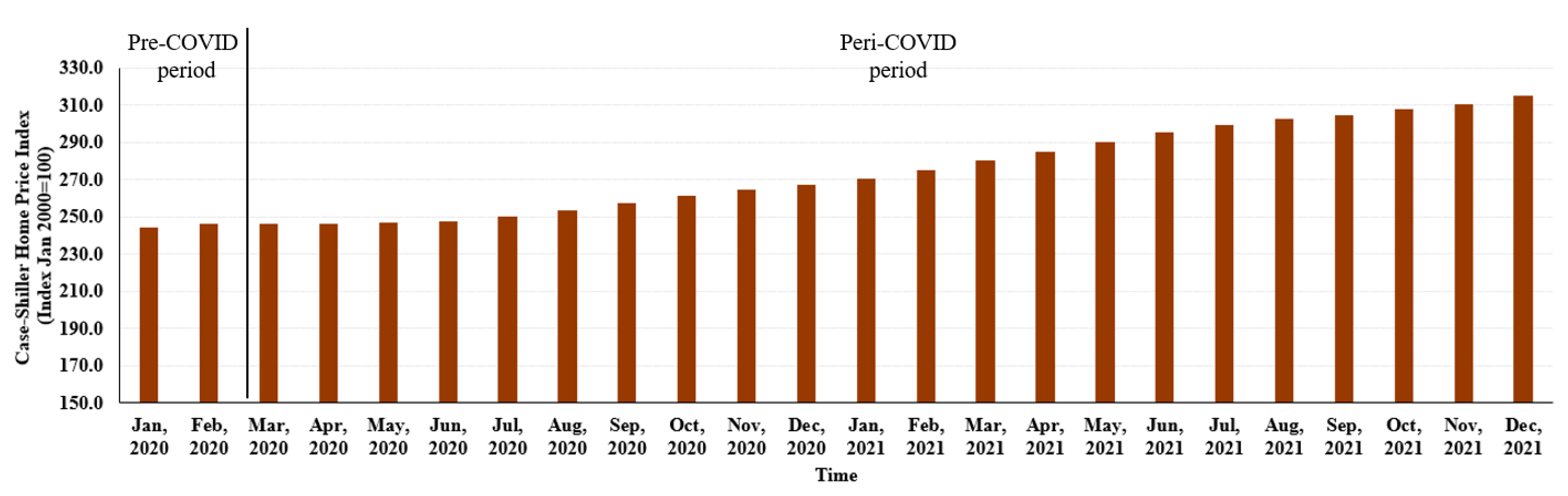
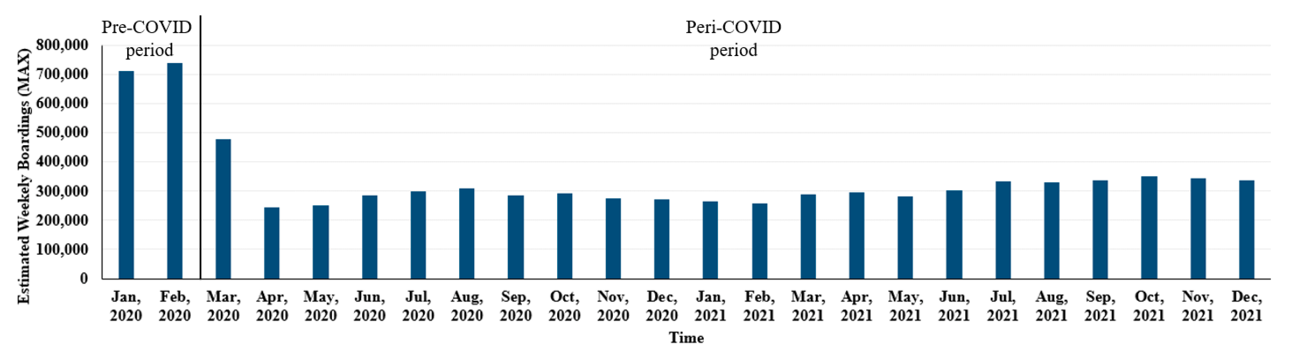
3.1.3. Broad Trends in Transit Ridership and Residential Property Values in Portland

Figure 1 and Figure 2 present the broad trends in transit ridership and residential property values for the Portland region in the pre- and peri-COVID periods. Figure 1 shows that before the pandemic, the estimated weekly boarding number for light rail transit was approximately 720,000. The LRT ridership decreased by around 35% in March 2020 and further declined by another 50% in April 2020. However, since April 2020, the ridership has stabilized, with an average of about 250,000 weekly boardings. The Case–Shiller home price index values in Figure 2 show an approximately 25% increase in home prices in the Portland area between January 2020 and November 2021, driven mainly by the Federal Reserve’s push for low-interest rates to mitigate the pandemic’s impact on the macro-economy.

3.2. Methodological Approach

Our methodological approach quantified the pandemic’s impact on the residential property value premium of light rail transit proximity (MAX in the Portland Metropolitan area) in the intermediate term by modeling homes near LRT stations as the treatment (treated) group in a quasi-experiment design. The impact is called the treatment effect in this paper. The treatment effect is the difference in the appreciation of home prices near stations and between the pre-COVID period (January 2016~February 2020) and the peri-COVID period (March 2020~December 2021).

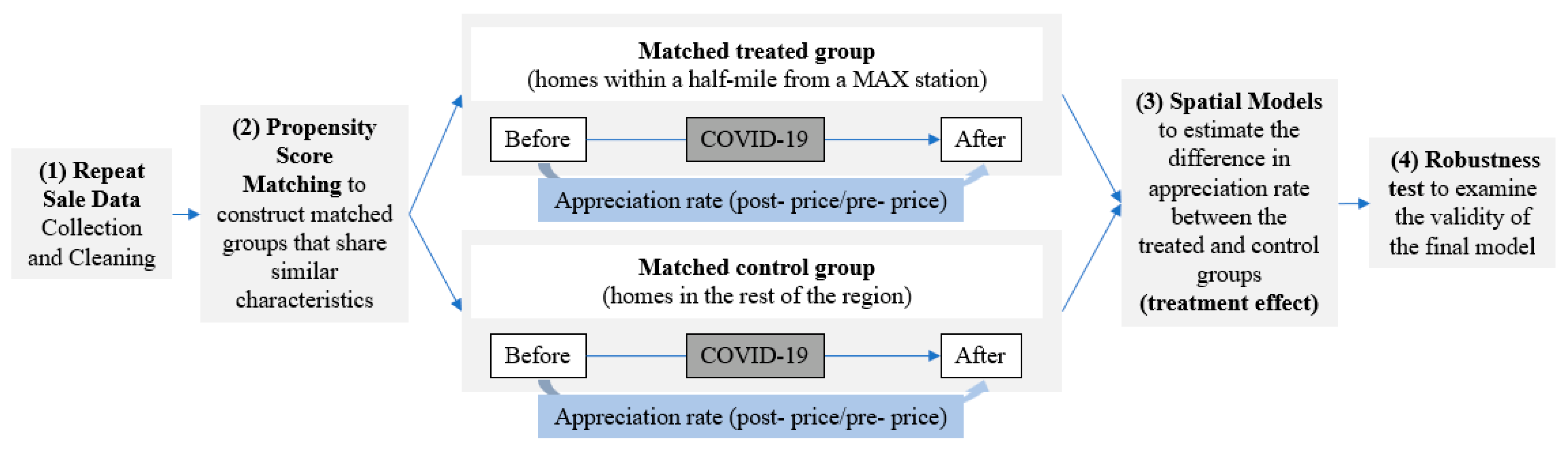
3.2.1. Overview of the Four-Step Process

We employed a four-step process of the longitudinal quasi-experimental design to estimate the treatment effects of single-family and multi-family homes (see Figure 3). We first collected and cleaned the home sales data and selected homes with at least one repeat sale between the pre-COVID and peri-COVID period. Second, we identified homes inside MAX station areas as the treated group and used a propensity score matching (PSM) method to identify homes outside station areas for the control group, whose characteristics matched those in the treated group. Third, we developed spatial models with the matched treated and control pairs to quantify the treatment effect. Finally, we conducted a robustness test to ensure the validity of the estimated treatment effect.

Our methodological approach has several advantages. First, the repeat sales data helped us alleviate the endogenous bias that mires traditional hedonic regression models [44]. Second, the PSM method approximates a randomized experiment [45,46], which addresses potential confounders by ensuring comparability across measured covariates between the treated and control groups [47]. Third, the spatial models control the spatial effects and overcome biases in the results for typical a-spatial hedonic models. Fourth, the robustness test validated our final results. We provide details on each step in the following subsections.

3.2.2. Step 1: Repeat Sales Data Collection and Cleaning

We used repeat sales data for single-family and multi-family homes in the Portland Metropolitan obtained from the Regional Land Information System (RLIS) of the Oregon Metro. Homes with one sale transaction in the pre-COVID period and one in the peri-COVID period were selected.

We cleaned the data with the following process. First, observations with missing sale price information were removed. Second, we used the same filter as Dong [48] and excluded transactions with sale prices lower than $50,000 (including records with sale prices equaling zero) or higher than $2 million, as such transactions were unlikely to occur in the study area. Third, we dropped properties that changed their primary characteristics, including the lot size, building size, and land use.

Lastly, we removed transaction records when the appreciation rate between the two periods was below the 2nd percentile or above the 98th percentile for the collected samples (e.g., around 1100% price change between the two periods) for the following reasons. Specifically, a critical assumption of a repeat sale analysis is that the innate characteristics of properties should not change throughout the study period. However, our data sources did not have information on the renovation, remodeling, or other improvements to a property. Additionally, it is important to rule out the impacts of other changes on the value, such as the increased quality of nearby schools and temporary closures of nearby amenities, which were not considered in our data set. Thus, we relied on the cut-off as a filter for properties with significant improvements between transactions. Moreover, because the repeat sales analysis approach is sensitive to extreme observations [49], we tried to exclude observations with extreme appreciation rates, such as the rate of around 1100% between the two periods.

3.2.3. Step 2: Propensity Score Matching

We used the propensity score matching (PSM) method to construct matched pairs of treated and control homes with similar observed characteristics and to overcome non-random assignment bias in the observational studies [50]. This step helped us to establish the direct causal effects of the intervention (the pandemic in our paper) on the outcomes.

Specifically, we used homes within a half-mile from their nearest MAX station, a common specification of previous studies on property value premiums [51], as observations in the treated group, while homes outside a half-mile buffer were in the candidate pool for the control group. The Portland region has a 14.7-mile commuter rail (WES) system serving Beaverton, Tigard, Tualatin, and Wilsonville. We excluded observations in the service area of the commuter rail system from the treated group, as the effect of the pandemic on commuter rail may differ from that on LRT.

We set a caliper width of 0.2 when identifying matched pairs for the unit in the treated group with the nearest-neighbors method. The caliper distance defines a tolerance level for the difference in propensity scores between the treated and the matched control group [52]. We used this caliper width for the following reasons. First, when using calipers with a width equal to 0.2, approximately 99% of the bias due to the measured confounders can be eliminated [53]. Additionally, a caliper width of 0.2 produced superior performance when estimating treatment effects in an experimental study by Wang et al. [52].

The covariates used to estimate the propensity scores included structural characteristics (e.g., lot size), locational factors (e.g., distance to central business district), and neighborhood characteristics (e.g., median household income).

Table 2. Descriptions of the covariates used in the propensity score matching.

Name	Description	Data Source
Treated	Dummy variable for whether the home is in the treated group, located within a half-mile from the nearest MAX (light rail transit system in the Portland metropolitan area) station	GIS
Structural Characteristics
Bldg Area	The building area of a home in square feet	RLIS
Lot Area	The lot area of a home in square feet	RLIS
Year Built	The year that a home was built	RLIS
Locational Factors
Freeway	Log-transformed distance in feet between each home and the nearest freeway at sale year during the pre-COVID period	GIS
Ramp	Log-transformed distance in feet between each home and the nearest ramp at sale year during the pre-COVID period	GIS
Bus	Log-transformed distance in feet between each home and the nearest bus stop at sale year during the pre-COVID period	GIS
CBD	Log-transformed distance in feet between each home and downtown (the City Hall of Portland) at sale year during the pre-COVID period [46]	GIS
Neighborhood Characteristics
Pop Den	The total population per acre at the census block group level at sale year during the pre-COVID period	ACS
White	The proportion of the residents who are non-Hispanic white at sale year during the pre-COVID period	ACS
HH Income	The median household income at the census block group level at sale year during the pre-COVID period	ACS
Education	The proportion of the population 25 years and over who attain less than high school at the census block group level at sale year during the pre-COVID period	ACS
Land Mix	The evenness in the spatial footprint of three land uses at census block group level at sale year during the pre-COVID period: residential, commercial/industrial, and others at sale year during the pre-COVID period $$land mix index=1-\left\{\frac{\left|\frac{r}{T}-\frac{1}{3}\right|+\left|\frac{c}{T}-\frac{1}{3}\right|+\left|\frac{o}{T}-\frac{1}{3}\right|}{4/3}\right\}$$ where $r$ is acres in residential use, $c$ is commercial/industrial use, $o$ is acres in other land uses, and T is $r+c+o$ [56].	GIS
Net Den	The total length of roads in feet per acre at the census block group level [57]	SLD
Intersect Den	The total length of street intersection per square mile at the census block group level [58]	SLD
School	The total number of schools per acre at the census block group level at sale year during the pre-COVID period	GIS
Access Auto	The number of jobs within 45 min auto travel time at the census block group level	SLD
Access Transit	The number of jobs within 45 min transit travel time at the census block group level	SLD

Sources. SLD: United States Environmental Protection Agency Smart Location Database version 3.0; ACS: American Community Survey 2016, 2017, 2018, and 2019 (the 5-year estimates); RLIS: the Regional Land Information System 2016, 2017, 2018, 2019, 2020, 2021, and 2022; GIS: shapefile data obtained from RLIS and calculated in ArcGIS.

below lists the 17 covariates used in PSM with a description and data source, while

Table 3. Descriptive statistics for the covariates used in the propensity score matching.

Name	Single-Family Housing			Multi-Family Housing
	N	Mean	Std. Dev	N	Mean	Std. Dev
Treated	4482	0.11	0.31	1319	0.27	0.44
Bldg Area	4482	1740.17	683.14	1319	1110.19	427.31
Lot Area	4482	5420.81	2268.88	1319	467.88	415.13
Year Built	4482	1976.68	33.58	1319	1986.70	24.06
Freeway	4482	12,350.99	13,784.36	1319	6696.87	11,124.49
Ramp	4482	29,708.26	23,426.22	1319	20,036.30	21,398.93
Bus	4482	4130.57	10,051.20	1319	1937.19	10,545.16
CBD	4482	49,321.33	28,259.63	1319	33,089.20	27,039.27
Pop Den	4482	5530.79	3332.20	1319	7810.15	6127.20
White	4482	80.38	12.06	1319	80.71	12.07
HH Income	4482	75,952.90	29,306.83	1319	73,756.83	27,919.97
Education	4482	8.21	7.26	1319	5.49	6.76
Land Mix	4482	0.42	0.20	1319	0.55	0.19
Net Den	4482	20.36	8.67	1319	25.09	10.23
Intersect Den	4482	125.96	79.70	1319	155.96	91.19
School	4482	1.15	1.47	1319	1.14	1.40
Access Auto	4482	63,692.91	29,062.29	1319	84,329.47	32,269.66
Access Transit	4482	46,730.84	88,329.29	1319	87,232.67	114,657.22

shows the descriptive statistics. For the covariate balance diagnostics, we used the standardized differences insensitive to the sample size [54] and paired t-tests [55].

3.2.4. Step 3: Spatial Econometrics Model

After finding matched pairs of treated and control groups, we used spatial lag (spatial autocorrelation, SAR) and a spatial error model (SEM) to account for the spatial autocorrelation [59,60] in estimating the treatment effect. We used the uniform kernel weight matrices; specifically, the average number of links was 84.54 in the model for single-family housing and 126.59 for multi-family housing.

The equation for SAR is as follows:

$$y={\beta }_0+{\beta }_1\ast T+{\beta }_2\ast Time+\beta X+\rho \mathsf{\omega }y+u$$

(1)

The SEM equation is as follows:

$$y={\beta }_0+{\beta }_1\ast T+{\beta }_2\ast Time+\beta X+ \mathsf{\gamma }\mathsf{\omega }ϵ+v$$

(2)

The dependent variable $y$ in both equations is the log-transformed appreciation rate of a home $y=\log (Pric{e}_{peri-COVID}/Pric{e}_{pre-COVID})$, which is a common practice in the previous literature with repeat sales data [20,23,48]. Our focus of the model was on estimating parameter ${\beta }_1$ (the treatment effect) for the dummy variable of matched treatment group $T$. We also controlled the length of time ($Time$) between two transactions to address seasonality. Lastly, we possibly needed to incorporate any covariates $X$ that were not perfectly matched via PSM. However, the results of balance diagnostics revealed no need to control for any covariates used during PSM.

The SAR and SEM approaches differ in how the error term is defined [61]. Specifically, in SAR, $\rho \mathsf{\omega }$ denotes the spatially lagged dependent variable $\rho$ (rho) for the weight matrix $\mathsf{\omega }$. In the SEM, $\mathsf{\gamma }$ denotes the spatial error parameter (lambda), $ϵ$ denotes the error term in the a-spatial model weighted by weight matrix $\mathsf{\omega }$, $u$ is a vector of error terms in the spatial lag model, and $v$ is the independent model error in the spatial error model [62,63].

Table 4. Descriptions of the covariates in spatial econometrics models.

Name	Description	Data Source
Dependent variable
ln(appreciation rate)	Log-transformed appreciation rate The appreciation rate was calculated as the sale price of a residential property during the COVID-19 pandemic (sold between March 2020 and December 2021) divided by the price of the same property before the COVID-19 outbreak (sold between January 2016 and February 2020).	RLIS
Independent variable
Treated	The dummy variable for a property located within a half-mile from the nearest MAX (light rail transit system in the Portland metropolitan area) station	RLIS
Length of time	Length of time between two transactions in months	RLIS

Source. RLIS: The Regional Land Information System 2016, 2017, 2018, 2019, 2020, 2021, 2022.

and

Table 5. Descriptive statistics for variables in spatial econometrics models.

Name	Single-Family Housing			Multi-Family Housing
	N	Mean	Std. Dev	N	Mean	Std. Dev
ln(appreciation rate)
Total sample	860	0.251	0.159	376	0.141	0.157
Matched Treated Group	430	0.249	0.153	188	0.127	0.155
Matched Control Group	430	0.253	0.165	188	0.156	0.158
Appreciation rate
Total sample	860	1.302	0.223	376	1.166	0.192
Matched Treated Group	430	1.300	0.213	188	1.150	0.182
Matched Control Group	430	1.310	0.233	188	1.180	0.202
Length of time
Total sample	860	42.5	12.5	376	41.5	12.7
Matched Treated Group	430	42.7	11.7	188	42.1	12.4
Matched Control Group	430	42.3	13.2	188	40.9	13.1

illustrate the covariates used in spatial econometrics models after data processing and PSM.

3.2.5. Step 4: Robustness Test

We tested whether our method and findings were robust in detecting changes in property value premiums over time in the Portland region in the absence of an exogenous shock such as the pandemic. This test was crucial to examine whether the treatment effect estimated in this paper was not due to the overall preference or trends in the housing market in the region.

We explored the effect of a hypothetical event happening on 1 January 2019. The method used here was identical to what we used throughout the paper for the pre-COVID and peri-COVID periods, except the dates for period 1 (the pre-hypothetical event) and period 2 (the peri-hypothetical event). The pre-hypothetical event period was between January 2016 and December 2018, while the peri-hypothetical event period was between January 2019 and February 2020.

4. Results

This section is divided into three subsections: (1) propensity score matching; (2) a spatial econometrics model; (3) a robustness test.

4.1. Propensity Score Matching

4.1.1. Balance Diagnostics

After the data cleaning process and propensity score matching (PSM) with a caliper width of 0.2, we obtained 860 single-family homes and 376 multi-family homes in matched treated and control groups (see Figure 4). Since none of the covariates were above 0.25 [64] in

Table 6. Results of standardized difference and paired t-tests between matched treated and control groups after propensity score matching.

Variables	Single-Family Housing		Multi-Family Housing
	Standardized Difference	p-Value of Paired t-Test	Standardized Difference	p-Value of Paired t-Test
Bldg Area	0.021	0.748	0.027	0.783
Lot Area	0.063	0.323	0.112	0.306
Year Built	0.015	0.798	0.056	0.475
Freeway	0.065	0.309	0.007	0.949
Ramp	0.019	0.714	0.013	0.878
Bus	0.026	0.769	0.024	0.846
CBD	0.088	0.182	0.019	0.825
Pop Den	0.015	0.828	0.039	0.481
White	0.036	0.571	0.121	0.250
HH Income	0.014	0.817	0.139	0.129
Education	0.010	0.876	0.040	0.740
Land Mix	0.091	0.225	0.137	0.170
Net Den	0.080	0.162	0.052	0.430
Intersect Den	0.062	0.325	0.059	0.339
School	0.041	0.5793	0.096	0.404
Access Auto	0.088	0.127	0.081	0.405
Access Transit	0.058	0.357	0.103	0.258
Sample Size	860 (430 pairs)		376 (188 pairs)

, the PSM performed well, and all covariates were balanced between the two matched groups. Furthermore, the p-values of the paired t-tests in Table 6 indicate that the pairs of observations in the matched treated and control groups showed no statistically significant difference across all 17 covariates in both housing markets. Thus, we constructed almost perfect matches and approximated random experiments, indicating no need to control for any of the covariates used in PSM when estimating the treatment effect in spatial econometrics models.

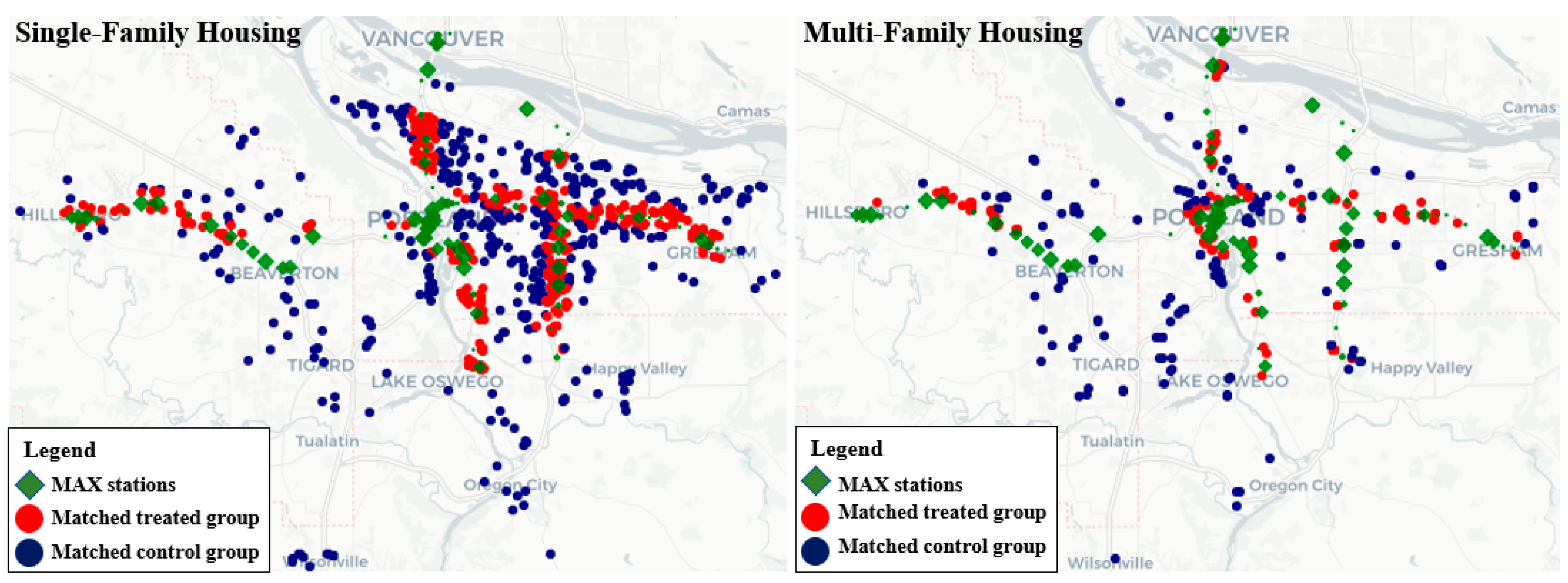
4.1.2. Descriptive Statistics of Matched Treated and Control Groups

Figure 5 shows the distributions of appreciation rates of single-family and multi-family homes in the two matched groups across the region. It visually reveals that single-family and multi-family homes with lower appreciation rates may be clustered near light rail transit (MAX in our study area) stations (green dots). Additionally, Table 5 indicates that the average appreciation rate for the treated group in both single-family and multi-family housing markets was lower than that of the control group. Specifically, the mean differences in log-transformed appreciation rates were −0.004 in the single-family housing market and −0.029 in the multi-family housing market.

4.2. Spatial Econometrics Model

4.2.1. Final Model Specification

Regarding the final model selection, we found that the spatial error model (SEM) performed better than the a-spatial (OLS) and spatial lag models (SAR) in both single-family and multi-family housing market analyses. First, Moran’s I [65] results revealed that the SEM and SAR performed better than the OLS due to the spatial dependency in the residuals (see

Table 7. The results of spatial autocorrelation checks.

	Moran’s I	Lagrange Multiplier (LM) Tests
		LM Test for Spatial Lag (LMlag)	LM Test for Spatial Error (LMerror)	Robust LM Test for Spatial Lag (RLMlag)	Robust LM Test for Spatial Error (RLMerror)	Portmanteau Test (SARMA)
Single-Family Housing	0.14 ***	27.34 ***	706.09 ***	1.19	679.90 ***	707.28 ***
Multi-Family Housing	0.26 ***	0.21	1611.80 ***	125.07 ***	1736.60 ***	1736.80 ***

* Significant at p < 0.10; ** significant at p < 0.05; *** significant at p < 0.01.

). More importantly, the Lagrange multiplier (LM) tests [66] in Table 7 indicate that the SEM was superior to the SAR due to the insignificant results for RLMlag in the single-family housing market and LMlag in the multi-family housing market. Furthermore, the lower values of the Akaike information criteria (AIC) in the SEM models support this conclusion. Therefore, we concluded that the SEM was a higher-order model, so we focused on interpreting the results from the SEM, although we include the results of the two other models for comparison in the following subsection.

4.2.2. Treatment Effect

Table 8. Results of the a-spatial, spatial lag, and spatial error models.

Housing Market	Single-Family Housing			Multi-Family Housing
Final Model	No	No	Yes	No	No	Yes
Models	OLS	SAR	SEM	OLS	SAR	SEM
	Estimate (Std. Error)	Total Impact (Std. Error)	Estimate (Std. Error)	Estimate (Std. Error)	Total Impact (Std. Error)	Estimate (Std. Error)
Constant	0.059 *** (0.019)	0.046 ** (0.018)	0.046 ** (0.018)	0.039 ** (0.028)	0.065 ** (0.029)	0.067 *** (0.025)
Treated	−0.006 (0.010)	−0.014 (0.010)	−0.008 (0.010)	−0.032 ** (0.016)	−0.031 ** (0.016)	−0.030 ** (0.013)
Length of time	0.005 *** (0.0004)	0.004 *** (0.0004)	0.005 *** (0.0004)	0.003 *** (0.001)	0.003 *** (0.001)	0.005 *** (0.001)
Model statistics
Observations	860	860	860	376	376	376
Adjusted R2	0.128			0.057
Rho		0.003 ***			−0.004
Lambda			0.013 ***			0.011 ***
Wald Statistics		19.846 ***	548.201 ***		4.403 **	907.491 ***
LR Test		20.538 ***	85.775 ***		1.196	156.509 ***
Log-likelihood		429.949	462.567		175.485	253.142
AIC	−831.360	−849.898	−915.135	−341.770	−340.970	−496.283

* Significant at p < 0.10; ** significant at p < 0.05; *** significant at p < 0.01. Models: a-spatial model (OLS), spatial lag model (SAR), and spatial error model (SEM).

shows the results of the a-spatial (OLS), spatial lag (SAR), and spatial error (SEM) models. In the single-family housing market, the estimated treatment effect indicates that observations in the treated group showed a negative but insignificant treatment effect compared to those in the matched control group (the zero-value default in the dummy variable). Conversely, the total impact of the treatment effect in the multi-family housing market was −0.030 with a lambda of 0.011. This suggests that the appreciation rate is 3.0 percent lower for a multi-family home located in a light rail transit service area than otherwise similar homes. Note that the negative value indicates the lower appreciation that multi-family homes near stations showed between the pre-COVID-period (January 2016~February 2020) and the peri-COVID-period (March 2020~December 2021), well after Portland’s LRT system had already been established and supposedly any property value premium from the LRT had already been reflected in the price. The estimated treatment effects of the OLS, SAR, and SEM were consistent in direction and significance.

4.3. Robustness Test

We conducted an additional analysis to explore whether our method would detect any changes in the premiums for single-family and multi-family homes without the pandemic shock. Here, we tested the effect of a hypothetical event happening on 1 January 2019.

Table 9. The results of robustness tests with a hypothetical exogenous shock.

Housing Market	Single-Family Housing			Multi-Family Housing
Final Model	No	No	Yes	No	No	Yes
Models	OLS	SAR	SEM	OLS	SAR	SEM
	Estimate (Std. Error)	Total Impact (Std. Error)	Estimate (Std. Error)	Estimate (Std. Error)	Total Impact (Std. Error)	Estimate (Std. Error)
Constant	0.314 *** (0.044)	0.218 *** (0.053)	0.253 *** (0.050)	0.103 * (0.061)	0.082 * (0.065)	0.152 ** (0.060)
Treated	0.023 (0.033)	0.018 (0.032)	0.020 (0.032)	0.027 (0.038)	0.028 (0.037)	0.031 (0.034)
Length of time	−0.004 ** (0.001)	−0.003 * (0.001)	−0.003 * (0.001)	0.001 (0.002)	0.001 (0.002)	0.002 (0.002)
Model statistics
Observations	194	194	194	78	78	78
Adjusted R2	0.023			0.011
Rho		0.012 ***			0.017
Lambda			0.020 **			0.070 ***
Wald Statistics		8.020 ***	10.374 ***		0.749	145.620 ***
LR Test		8.862 ***	5.345 **		0.601	14.521 ***
Log-likelihood		17.806	16.047		30.341	37.301
AIC	−18.749	−25.611	−22.094	−52.080	−50.681	−64.601

Notes. Pre-hypothetical event: January 2016~December 2018; post-hypothetical event: 01/2019~02/2020. * Significant at p < 0.10; ** significant at p < 0.05; *** significant at p < 0.01. Models: a-spatial model (OLS), spatial lag model (SAR), and spatial error model (SEM).

below reveals that none of the treatment effects were significant even at the 0.1 significance level in the OLS, SAR, and SEM, indicating our method did not estimate a significant change in the premium for LRT absent of the pandemic. This result proves that the estimated treatment effect in Table 8 is robust.

5. Discussions

5.1. Single-Family Housing Market

We found an insignificant effect of the pandemic on the prices of single-family homes near LRT stations. This finding deserves further discussion. Florida et al. [67] argued that the pandemic might lead to a series of changes in the short term at the neighborhood level due to social scarring, the lockdown, the need for measures against future health risks, and changed preferences in the urban built environment. However, it is unlikely to change long-standing spatial patterns. Although COVID-19 has influenced our daily lives, such as reduced transit ridership and changed residential location preferences, our result suggests that in the intermediate term, transit proximity has not significantly changed its appeal in the single-family housing market.

Additionally, homebuyers may think that the disruptions from the COVID-19 pandemic, even though dramatic and swift, will be short-lived. If they perceive the pandemic as a short-term disruption, the location preference established over a long time may not change in a significant way. Furthermore, well after Portland’s LRT system was established, and supposedly any property value premium for the LRT had already been reflected in the price, significant disruptions such as the COVID pandemic did not significantly impact the LRT premium.

Furthermore, Tan and Ma [68] examined how personal attributes, travel attributes, and the perception of COVID-19 influenced choosing rail transit in a hypothetical situation where people were resuming their work in the post-COVID 19 era. They found that the walking time from home to the nearest transit station would negatively impact the commuter’s choice of rail transit; that is, the research implies that a shorter walking time to the transit station would not lose its appeal in the single-family housing market, given the insignificant impact of the pandemic.

5.2. Multi-Family Housing Market

Conversely, the significant negative effect on multi-family homes proximate to transit stations indicates that they were slightly losing their premium during the pandemic. The COVID-19 outbreak has generated unusual travel behavior changes, particularly regarding transit use. For instance, people would likely favor private vehicles rather than public transit in the post-COVID-19 era [3] because they tend to reduce risk-taking behavior when living through risk events [69]. For instance, nearly 70% of transit riders have changed their travel behavior during the pandemic in the Portland region (see Figure 1). Therefore, we believe that it may disrupt the demand for multi-family homes, resulting in decreased property values, as transit service areas generally represent a market with multi-family housing demands sensitive to proximity to amenities and social services.

Moreover, the finding suggests that in the multi-family housing markets in the region, the impact of the pandemic did not become “decoupled” from the transit utility, as the actual ridership volume significantly declined, while the property premiums did decrease considerably. Specifically, due to the significant decline in transit ridership, the proximity that offers transit users more convenience, easy access to transit, and a lower probability of contacting people on the journey to that station may not be important in the multi-family housing market.

6. Conclusions

Whether the preference for neighborhoods with better transit accessibility remained during the pandemic was a research question that had not been investigated. To fill this gap, we used repeat sales data with a quasi-experimental design that would allow us to establish a causal relationship (if the assumptions of our models are reasonable). We found different results for the single-family and multi-family housing markets. Specifically, during the COVID-19 pandemic, single-family homes within a half-mile from the nearest station showed an insignificant difference in the appreciation rate compared to those with similar characteristics. In contrast, multi-family homes within a half-mile from the nearest station received a 3.0% lower appreciation rate than homes with similar characteristics. Moreover, the robustness test offered evidence that the findings were robust. We believe our study contributes to a growing body of knowledge about the property value premiums associated with LRT proximity and COVID-induced disruptions in our life. Additionally, the findings will help broaden the discussion regarding the changes in post-COVID cities and their planning implications.

We acknowledge a few limitations of this study. First, our analysis did not consider other changes due to the pandemic, such as temporarily closed amenities and unemployment. This may be problematic if the pandemic affects the LRT service area differently (besides the prices) than the rest of the region. Second, our data source does not provide common home attributes, including the numbers of bedrooms and bathrooms or interior design details. Third, our models did not include all factors that homebuyers value when on the housing market, such as school quality and other amenities. Fourth, we do not know how generalizable our results from the Portland area are to other regions in the U.S., let alone across the globe.

For future research, in addition to addressing the limitations listed above when better data become available, we plan to revisit this study with updated data to estimate the longer-term effect of the pandemic. Additionally, since our analysis did not address the relationship between the decreased transit ridership and property value premium, further research is needed to explore this connection.

References

1. Tanrıvermiş, H. Possible Impacts of COVID-19 Outbreak on Real Estate Sector and Possible Changes to Adopt: A Situation Analysis and General Assessment on Turkish Perspective. J. Urban Manag. 2020, 9, 263–269. [Google Scholar] [CrossRef]
2. Yin, Y.; Li, D.; Zhang, S.; Wu, L. How Does Railway Respond to the Spread of COVID-19? Countermeasure Analysis and Evaluation Around the World. Urban Rail Transit 2021, 7, 29–57. [Google Scholar] [CrossRef] [PubMed]
3. Honey-Rosés, J.; Anguelovski, I.; Chireh, V.K.; Daher, C.; Bosch, C.K.; van den Litt, J.S.; Mawani, V.; McCall, M.K.; Orellana, A.; Oscilowicz, E.; et al. The Impact of COVID-19 on Public Space: An Early Review of the Emerging Questions–Design, Perceptions and Inequities. Cities Health 2020, 5, S263–S279. [Google Scholar] [CrossRef]
4. Nanda, A.; Thanos, S.; Valtonen, E.; Xu, Y.; Zandieh, R. Forced Homeward: The COVID-19 Implications for Housing. Town Plan. Rev. 2021, 92, 25–31. [Google Scholar] [CrossRef]
5. Zhang, D.; Jiao, J. How Does Urban Rail Transit Influence Residential Property Values? Evidence from An Emerging Chinese Megacity. Sustainability 2019, 11, 534. [Google Scholar] [CrossRef] [Green Version]
6. Siripanich, A.; Rashidi, T.H.; Moylan, E. Interaction of Public Transport Accessibility and Residential Property Values Using Smart Card Data. Sustainability 2019, 11, 2709. [Google Scholar] [CrossRef] [Green Version]
7. Gong, W.; Li, J.; Ng, M.K. Deciphering Property Development around High-Speed Railway Stations through Land Value Capture: Case Studies in Shenzhen and Hong Kong. Sustainability 2021, 13, 12605. [Google Scholar] [CrossRef]
8. Dawkins, C.; Moeckel, R. Transit-Induced Gentrification: Who Will Stay, and Who Will Go? Hous. Policy Debate 2016, 26, 801–818. [Google Scholar] [CrossRef]
9. Bartholomew, K.; Ewing, R. Hedonic Price Effects of Pedestrian- and Transit-Oriented Development. J. Plan. Lit. 2011, 26, 18–34. [Google Scholar] [CrossRef]
10. Alonso, W. A Theory of the Urban Land Market. In Urban and Regional Economics; 1960; pp. 83–91. Available online: http://lib.cufe.edu.cn/upload_files/other/4_20140526030430_59_A%20theory%20of%20the%20urban%20land%20market.pdf (accessed on 19 June 2022).
11. Mills, E.S. Studies in the Structure of the Urban Economy; John Hopkins Press: Baltimore, MD, USA, 1972. [Google Scholar]
12. Muth, R.F. Cities and Housing; the Spatial Pattern of Urban Residential Land Use; University of Chicago Press: Chicago, IL, USA, 1969. [Google Scholar]
13. Wingo, L. Transportation and Urban Land, 1st ed.; Routledge: London, UK, 1961; ISBN 978-1-138-96267-5. [Google Scholar]
14. Bowes, D.R.; Ihlanfeldt, K.R. Identifying the Impacts of Rail Transit Stations on Residential Property Values. J. Urban Econ. 2001, 50, 1–25. [Google Scholar] [CrossRef]
15. Duncan, M. Comparing Rail Transit Capitalization Benefits for Single-Family and Condominium Units in San Diego, California. Transp. Res. Rec. 2008, 2067, 120–130. [Google Scholar] [CrossRef]
16. Pan, Q. The Impacts of an Urban Light Rail System on Residential Property Values: A Case Study of the Houston METRORail Transit Line. Transp. Plan. Technol. 2013, 36, 145–169. [Google Scholar] [CrossRef]
17. Cervero, R.; Duncan, M. Benefits of Proximity to Rail on Housing Markets: Experiences in Santa Clara County. J. Public Transp. 2002, 5, 1–18. [Google Scholar] [CrossRef] [Green Version]
18. Hess, D.B.; Almeida, T.M. Impact of Proximity to Light Rail Rapid Transit on Station-Area Property Values in Buffalo, New York. Urban Stud. 2007, 44, 1041–1068. [Google Scholar] [CrossRef]
19. Hamidi, S.; Kittrell, K.; Ewing, R. Value of Transit as Reflected in U.S. Single-Family Home Premiums: A Meta-Analysis. Transp. Res. Rec. 2016, 2543, 108–115. [Google Scholar] [CrossRef]
20. Chatman, D.G.; Tulach, N.K.; Kim, K. Evaluating the Economic Impacts of Light Rail by Measuring Home Appreciation: A First Look at New Jersey’s River Line. Urban Stud. 2012, 49, 467–487. [Google Scholar] [CrossRef]
21. McIntosh, J.; Trubka, R.; Newman, P. Can Value Capture Work in a Car Dependent City? Willingness to Pay for Transit Access in Perth, Western Australia. Transp. Res. Part A Policy Pract. 2014, 67, 320–339. [Google Scholar] [CrossRef]
22. He, S.Y. Regional Impact of Rail Network Accessibility on Residential Property Price: Modelling Spatial Heterogeneous Capitalisation Effects in Hong Kong. Transp. Res. Part A Policy Pract. 2020, 135, 244–263. [Google Scholar] [CrossRef]
23. Kim, K.; Lahr, M.L. The impact of Hudson-Bergen Light Rail on residential property appreciation. Pap. Reg. Sci. 2014, 93, S79–S97. [Google Scholar] [CrossRef] [Green Version]
24. Cao, X.; Lou, S. When and How Much Did the Green Line LRT Increase Single-Family Housing Values in St. Paul, Minnesota? J. Plan. Educ. Res. 2018, 38, 427–436. [Google Scholar] [CrossRef]
25. Song, Z.; Cao, M.; Han, T.; Hickman, R. Public Transport Accessibility and Housing Value Uplift: Evidence from the Docklands Light Railway in London. Case Stud. Transp. Policy 2019, 7, 607–616. [Google Scholar] [CrossRef]
26. Lee, S.; Wang, L.; Dong, H.; Yang, H. Temporal Dynamics of the Effects of Light Rail on the Housing Prices: A Case Study of Portland, Oregon. Available online: http://wstlur.org/symposium/2021/documents/WSTLUR_2021_Abstract_Book_June24.pdf (accessed on 10 June 2021).
27. Knaap, G.J.; Ding, C.; Hopkins, L.D. Do Plans Matter?: The Effects of Light Rail Plans on Land Values in Station Areas. J. Plan. Educ. Res. 2001, 21, 32–39. [Google Scholar] [CrossRef]
28. Agostini, C.A.; Palmucci, G.A. The Anticipated Capitalisation Effect of a New Metro Line on Housing Prices. Fisc. Stud. 2008, 29, 233–256. [Google Scholar] [CrossRef]
29. Jayantha, W.M.; Lam, T.I.; Chong, M.L. The Impact of Anticipated Transport Improvement on Property Prices: A Case Study in Hong Kong. Habitat Int. 2015, 49, 148–156. [Google Scholar] [CrossRef]
30. Golub, A.; Guhathakurta, S.; Sollqpuram, B. Spatial and Temporal Capitalization Effects of Light Rail in Phoenix: From Conception, Planning, and Construction to Operation. J. Plan. Educ. Res. 2012, 32, 415–429. [Google Scholar] [CrossRef]
31. Pearson, J.; Muldoon-Smith, K.; Liu, H.; Robson, S. How Does the Extension of Existing Transport Infrastructure Affect Land Value? A Case Study of the Tyne and Wear Light Transit Metro System. Land Use Policy 2022, 112, 105811. [Google Scholar] [CrossRef]
32. Yan, S.; Delmelle, E.; Duncan, M. The Impact of a New Light Rail System on Single-Family Property Values in Charlotte, North Carolina. J. Transp. Land Use 2012, 5, 60–67. [Google Scholar] [CrossRef] [Green Version]
33. Ke, Y.; Gkritza, K. Light Rail Transit and Housing Markets in Charlotte-Mecklenburg County, North Carolina: Announcement and Operations Effects Using Quasi-Experimental Methods. J. Transp. Geogr. 2019, 76, 212–220. [Google Scholar] [CrossRef]
34. Liu, L.; Miller, H.J.; Scheff, J. The Impacts of COVID-19 Pandemic on Public Transit Demand in the United States. PLoS ONE 2020, 15, e0242476. [Google Scholar] [CrossRef]
35. Brough, R.; Freedman, M.; Phillips, D. Understanding Socioeconomic Disparities in Travel Behavior during the COVID-19 Pandemic; Social Science Research Network: Rochester, NY, USA, 2020. [Google Scholar]
36. Hu, S.; Chen, P. Who Left Riding Transit? Examining Socioeconomic Disparities in the Impact of COVID-19 on Ridership. Transp. Res. Part D Transp. Environ. 2021, 90, 102654. [Google Scholar] [CrossRef]
37. WMATA. Metro and COVID-19: Steps We’ve Taken | WMATA. Available online: https://www.wmata.com/service/covid19/COVID-19.cfm (accessed on 26 May 2021).
38. Jung, H. The Impact of an Epidemic on Transit Ridership. J. Public Transp. 2020, 22, 1. [Google Scholar] [CrossRef]
39. Ramani, A.; Bloom, N. The Donut Effect: How COVID-19 Shapes Real Estate; Standford Institute for Economic Policy Research: Standford, CA, USA, 2021; p. 8. [Google Scholar]
40. Liu, S.; Su, Y. The Impact of the COVID-19 Pandemic on the Demand for Density: Evidence from the U.S. Housing Market; Social Science Research Network: Rochester, NY, USA, 2021. [Google Scholar]
41. TriMet. TriMet Service and Ridership Information. Available online: https://trimet.org/about/pdf/trimetridership.pdf (accessed on 30 November 2020).
42. D’Lima, W.; Lopez, L.A.; Pradhan, A. COVID-19 and Housing Market Effects: Evidence from U.S. Shutdown Orders; Social Science Research Network: Rochester, NY, USA, 2020. [Google Scholar]
43. Yoruk, B. Early Effects of the COVID-19 Pandemic on Housing Market in the United States; Social Science Research Network: Rochester, NY, USA, 2020. [Google Scholar]
44. Sun, W.; Zheng, S.; Wang, R. The Capitalization of Subway Access in Home Value: A Repeat-Rentals Model with Supply Constraints in Beijing. Transp. Res. Part A Policy Pract. 2015, 80, 104–115. [Google Scholar] [CrossRef]
45. Concato, J.; Shah, N.; Horwitz, R.I. Randomized, Controlled Trials, Observational Studies, and the Hierarchy of Research Designs. N. Engl. J. Med. 2000, 342, 1887–1892. [Google Scholar] [CrossRef] [PubMed] [Green Version]
46. Dong, H. Rail-Transit-Induced Gentrification and the Affordability Paradox of TOD. J. Transp. Geogr. 2017, 63, 1–10. [Google Scholar] [CrossRef]
47. Ali, M.S.; Prieto-Alhambra, D.; Lopes, L.C.; Ramos, D.; Bispo, N.; Ichihara, M.Y.; Pescarini, J.M.; Williamson, E.; Fiaccone, R.L.; Barreto, M.L.; et al. Propensity Score Methods in Health Technology Assessment: Principles, Extended Applications, and Recent Advances. Front. Pharmacol. 2019, 10, 973. [Google Scholar] [CrossRef]
48. Dong, H. Were Home Prices in New Urbanist Neighborhoods More Resilient in the Recent Housing Downturn? J. Plan. Educ. Res. 2015, 35, 5–18. [Google Scholar] [CrossRef] [Green Version]
49. Zhang, L.; Yi, Y. Quantile House Price Indices in Beijing. Reg. Sci. Urban Econ. 2017, 63, 85–96. [Google Scholar] [CrossRef]
50. Rosenbaum, P.R.; Rubin, D.B. The Central Role of the Propensity Score in Observational Studies for Causal Effects. Biometrika 1983, 70, 41–55. [Google Scholar] [CrossRef]
51. Landis, J.; Guhathakurta, S.; Huang, W.; Zhang, M.; Fukuji, B. Rail Transit Investments, Real Estate Values, and Land Use Change: A Comparative Analysis of Five California Rail Transit Systems. 1995. Available online: https://escholarship.org/uc/item/4hh7f652 (accessed on 19 June 2022).
52. Wang, Y.; Cai, H.; Li, C.; Jiang, Z.; Wang, L.; Song, J.; Xia, J. Optimal Caliper Width for Propensity Score Matching of Three Treatment Groups: A Monte Carlo Study. PLoS ONE 2013, 8, e81045. [Google Scholar] [CrossRef] [Green Version]
53. Austin, P.C. An Introduction to Propensity Score Methods for Reducing the Effects of Confounding in Observational Studies. Multivar. Behav Res 2011, 46, 399–424. [Google Scholar] [CrossRef] [Green Version]
54. Kelley, K.; Rausch, J.R. Sample Size Planning for the Standardized Mean Difference: Accuracy in Parameter Estimation via Narrow Confidence Intervals. Psychol. Methods 2006, 11, 363–385. [Google Scholar] [CrossRef] [PubMed] [Green Version]
55. Hsu, H.; Lachenbruch, P.A. Paired t Test. In Encyclopedia of Biostatistics; American Cancer Society: Atlanta, GA, USA, 2005; ISBN 978-0-470-01181-2. [Google Scholar]
56. Bhat, C.R.; Gossen, R. A Mixed Multinomial Logit Model Analysis of Weekend Recreational Episode Type Choice. Transp. Res. Part B Methodol. 2004, 38, 767–787. [Google Scholar] [CrossRef] [Green Version]
57. Gehrke, S.R.; Wang, L. Operationalizing the Neighborhood Effects of the Built Environment on Travel Behavior. J. Transp. Geogr. 2020, 82, 102561. [Google Scholar] [CrossRef]
58. Ewing, R.; Tian, G.; Goates, J.; Zhang, M.; Greenwald, M.J.; Joyce, A.; Kircher, J.; Greene, W. Varying Influences of the Built Environment on Household Travel in 15 Diverse Regions of the United States. Urban Stud. 2015, 52, 2330–2348. [Google Scholar] [CrossRef]
59. Anselin, L. Spatial Econometrics. In A Companion to Theoretical Econometrics; Baltagi, B.H., Ed.; Blackwell Publishing Ltd.: Malden, MA, USA, 2003; pp. 310–330. ISBN 978-0-470-99624-9. [Google Scholar]
60. Anselin, L. Spatial Econometrics: Methods and Models; Springer Science & Business Media: Berlin, Germany, 2013; ISBN 978-94-015-7799-1. [Google Scholar]
61. LeSage, J.P. An Introduction to Spatial Econometrics. Revue D’économie Industrielle 2008, 123, 19–44. Available online: https://econpapers.repec.org/article/caireidbu/rei_5f123_5f0019.htm (accessed on 19 June 2022). [CrossRef] [Green Version]
62. Conway, D.; Li, C.Q.; Wolch, J.; Kahle, C.; Jerrett, M. A Spatial Autocorrelation Approach for Examining the Effects of Urban Greenspace on Residential Property Values. J. Real. Estate. Financ. Econ. 2010, 41, 150–169. [Google Scholar] [CrossRef]
63. Liu, J.H.; Shi, W. Impact of Bike Facilities on Residential Property Prices. Transp. Res. Rec. 2017, 2662, 50–58. [Google Scholar] [CrossRef] [Green Version]
64. Rubin, D.B. Using Propensity Scores to Help Design Observational Studies: Application to the Tobacco Litigation. Health Serv. Outcomes Res. Methodol. 2001, 2, 169–188. [Google Scholar] [CrossRef]
65. Moran, P.A.P. Notes on Continuous Stochastic Phenomena. Biometrika 1950, 37, 17–23. [Google Scholar] [CrossRef]
66. Anselin, L. Lagrange Multiplier Test Diagnostics for Spatial Dependence and Spatial Heterogeneity. Geogr. Anal. 1988, 20, 1–17. [Google Scholar] [CrossRef]
67. Florida, R.; Rodríguez-Pose, A.; Storper, M. Cities in a Post-COVID World. Urban Stud. 2021, 23. [Google Scholar] [CrossRef]
68. Tan, L.; Ma, C. Choice Behavior of Commuters’ Rail Transit Mode during the COVID-19 Pandemic Based on Logistic Model. J. Traffic Transp. Eng. Engl. Ed. 2021, 8, 186–195. [Google Scholar] [CrossRef]
69. Cooper, T.; Faseruk, A. Strategic risk, Risk Perception and Risk Behaviour: Meta-Analysis. J. Financ. Manag. Anal. 2011, 24, 20–29. [Google Scholar]
Figure 1. Estimated weekly boardings of light rail transit in the Portland Metropolitan Area (Source: TriMet, Portland).
Sustainability 14 09107 g001
Figure 2. The monthly Case–Shiller home price index of the Portland metropolitan area (Adapted with permission from July 24, 2022, S&P Dow Jones Indices LLC, S&P/Case-Shiller OR-Portland Home Price Index [POXRSA], retrieved from FRED, Federal Reserve Bank of St. Louis; https://fred.stlouisfed.org/series/POXRSA).
Sustainability 14 09107 g002
Figure 3. The four-step process of the longitudinal quasi-experiment design.
Sustainability 14 09107 g003
Figure 4. The locations of observations in matched treated and control groups.
Sustainability 14 09107 g004
Figure 5. The appreciation rates of observations in matched treated and control groups.
Sustainability 14 09107 g005