Performance Loss Rates of a 1 MWp PV Plant with Various Tilt Angle, Orientation and Installed Environment in the Capital of Cyprus

Abstract

Evolution from fossil fuel sources to environmentally friendly and sustainable energy sources is one of the key aspects of the energy transition goal. On the other hand, Solar Photovoltaic systems are the most promising and improving technologies in the energy market However, it is well known that the performance of PV panels decreases in the process of time. This paper focuses on analyzing the performance loss rates (PLR) of mid-scale crystalline silicon (c-Si) PV systems of the same manufacturer with different orientations and tilt angles in the same region for the duration of four years of outdoor exposure. Three commonly used statistical methods are deployed to calculate PLRs; seasonal and trend decomposition using locally weighted scatterplot smoothing (STL), classical seasonal decomposition (CSD) and year on year (YoY) methods coupled with various performance metrics, namely Performance ratio (PR), temperature corrected performance ratio TCPR) and weather corrected performance ratio suggested by National Renewable Energy Laboratory (NRELPR). It is found that PLRs of analyzed venues, Arazi, Arena and Stonite, with the YOY approach are −1.2%/year, −0.73%/year and −2.65%/year, respectivelty., respectively. Furthermore, STL method demonstrated PLRs of −0.69%/year, −0.65%/year and −2.91%/year, respectively. On the other hand, the CSD method generated positive PLRs for some inverters while aforementioned statistical approaches proposed PLRs close to −2%/year, making the CSD method inappropriate for use under a heavy soiling environment. Within two km distance, variations up-to four-fold in PLRs are recorded between the venues during analyzed period. Furthermore, variations in PLRs are more dependent on the statistical approach rather than the performance metric.

1. Introduction

In a fast-changing global energy market, the demand for electricity is rising more than ever. According to IEA’s semiannual Electricity Market Report, the global electricity demand has risen 6% in 2021, largest increase in percentage terms since 2010 [1]. The gradual electrification of transport sector also will add stress to utility markets specifically in isolated grids. Solar energy technologies (photovoltaics (PV), solar collectors) are particular interest to North Cyprus due to the global horizontal irradiation (GHI) reaching 5.5 kWh/m² [2]. The cumulative global installed PV capacity is estimated to reach 760 GW, with an additional capacity of 130 GW in 2020, passing cumulative global installed Wind capacity for the first time [3]. Similarly cumulative installed PV capacity in North Cyprus has reached 95 MW by the end of 2021, reaching 25% of the total installed conventional capacity and the total electricity generation from photovoltaics has exceeded 10% of the total electricity generation [4].

With the increased cumulative installed PV capacity, the island’s isolated grid is facing severe issues. Alongside the voltage rise issues in low voltage grid due to concentrated PV installations in some areas, the lack of demand for electricity specially in late April is the main limitation for PV integration. Considering island’s limited grid capacity, the ability to predict the decline in power output from photovoltaics over the time holds significant importance for maximizing the renewables share in energy mix.

Over the years, two terms used to represent the decline in power output of a PV system over the time degradation rate and performance loss rate (PLR) often represented with a unit of %/year. PLR incorporates both reversible components i.e., soiling, shading, degradation in balance of system (BOS) components and irreversible components, and material degradation of modules [5], while the degradation rate only incorporates the irreversible component. Performance metrics used for degradation/PLR determination in the literature may be broadly categorized into three based on the monitored parameters; namely electrical parameters, regression models and normalized ratings. Based on the selected performance metric, it is either called performance loss rates (PLRs) or degradation rates of PV module or system [6]. Generally, the assessment of short circuit current I_sc, open-circuit voltage V_oc, fill factor FF and efficiency analysis leads determination of degradation rates since both indoor and outdoor analysis technique allows for the cleaning of module prior to parameter measurements. This is followed by a comparison of instantaneous measured parameters to the nameplate of module for determining the power reduction. On the other hand, Regression models and normalized ratings are based on the field data. Field data provides aggregated values, includes soiling, shading, module mismatch in addition to the degradation of PV modules, therefore represented by performance loss rate. Degradation/PLR determined by field measurements do not provide any information related to degradation modes. The severity of degradation/PLR of field aged PV systems is highly dependent on external conditions such as solar radiation, temperature, wind speed, humidity and soiling and evidenced by the observed degradations such as delamination, glass breakage, busbar failure, broken interconnect, front surface discoloration, moisture ingress, reduced interlayer adhesion, diode failure, hotspots, corrosion, contact stability, cracked cells etc. [7,8,9,10,11,12,13]. In addition to external conditions, it is also dependent on PV technology [14], data quality [15], filtering steps [15], aggregation period [16], performance metric [17], and statistical approaches [14,17]. On the other hand, accelerated indoor aging tests conducted in a controlled environment provide flexibility for determining the impact of parameters on degradation rates such as irradiation, temperature etc. Various procedures including damp-heat (DH), thermal cycling (TC), UV exposure, mechanical load etc. are developed to mimic real environmental conditions for testing the degradation rate of PV modules [6].

Various studies have reported PLR/Degradation rate for both natural and induced aged PV modules. Khan et al., conducted TC stress test composed of 200 cycles by varying temperature between −40 °C to 85 °C for PV modules, one fixed on a concrete slab, protecting the back surface of PV module while the other was left unprotected under controlled environment. Results suggested power loss for the reference PV module was approximately 3%, while concrete insulated PV modules only experienced a power loss of around 2% [18]. Kyranaki et al., conducted experimental study to investigate the front and read side corrosion mechanisms by subjecting 3 set of c-si mini modules, one set of full module structure of glass-EVA-cell-EVA-backsheet being the control and the other two sets having either front or rear side exposed to damp-heat conditioning under 85% relative humidity (RH) and 85 °C. Results revealed that for the front side exposure Pmax was observed to drop by an average of 4.65%. On the other hand, for the rear-side exposed PV cells Pmax dropped by 9.3% while maximum power output of full modules degraded by 5.6%. Front side corrosion was the dominant form of degradation mode, mostly on the fingers and busbars and less on solder of the ribbons [19]. Wu et al., conduced statistical analysis studies on UV induced degradation rate of polysilicon modules tested based on IEC 61215:2005. Results suggested after 3000 kWh/m² UV exposure, 95% of the tested modules did not exceed 8% degradation rate. Concluding, UV-induced degradation should not exceed 8% after 25 years of exposure [20].

PLR/degradation rates studies for modules exposed to outdoor conditions presented in literature are summarized in

Table 1. Illustrating reported PLR/Degradation rates.

Country	Duration (Years)	Capacity	Module Type	Mean Annual Degradation Rate	Degradation Methodology	Statistical Approach	Reference
Djibouti	5	302.4 kWp	Polycrystalline	PVUSA 0.96%/year & PR 1.01%	PVUSA & PR	Linear regression	Hassan Daher et al. (2022) [28]
USA	2–16	40 module	Mono-Polycrystalline	Mono 0.5%-poly 0.6%	PVUSA	ANOVA	Jordan et al. (2010) [29]
Florida USA	2.5–5	1.98–5940 kWp	Mono-Polycrystalline	PR 1.23/year & PVUSA 1.70%	PV USA & PR	Linear regression	Sorloaica et al. (2012) [30]
Cyprus	2	1 kWp	Mono-Polycrystalline	Multi PR 0.03% & PVUSA 0.63. MONO PR 0.02% & PVUSA 0.47%	PVUSA & PR		Makrides et al. [31]
Morocco	6	2.04 kWp	Mono- Polycrystalline	0.53% & 0.41% for mono 0.36% & 0.2% poly	PR corrected	LR & CSD	Ameur et al. (2022) [24]
Algeria	3	Module based	Mono-polycrystalline	0.83% for poly & 0.79% for mono	PR corrected	-	Silvestre et al. (2018) [25]
Cyprus	5	Module based	Mono-Poly-Thinfilm etc.	PR LLS 0.65-PR TC LLS 1.04	PR & PR corrected	LLS-CSD-STL	Phinikarides et al. 2013 [14]
Zurich	10	3450 kWp	Poly-Crystalline	0.50%	PR corrected	-	Carigiet et al. 2021 [27]
USA	5	8 MWp	Monocrystalline	1.10%	Pr corrected	YOY	Paudyal et al. 2020 [16]
Germany-Cyprus	7	1 kWp	Mono-polycrystalline	0.1–1%	PR	YOY ARIMA OLS CSD STL RCPA	Frick et al. (2020) [15]
UK & Australia	10	3.960 kWp	Polycrystalline	1.05–1.16 UK & 1.35–1.46 Australia	PR corrected	YOY	Dhimish et al. (2020) [10]
Italy & Australia	6	module based	Monocrystalline	0.95 Bolzano & 0.80 Australia & 2.21 Milano & 0.63 Catania	PR	STL	P. Ingenhoven (2019) [22]
Italy & Australia & Indonesia	2–9	20 kwp	polycrystalline	0.6/years	PR	YOY & STL	Kunaifi et al. (2020) [32]
İndia	4	1 MWP	monocrystalline	0.27 LLS & 0.32 CSD & 0.50 HW & 0.27 STL	PR	LLS-CSD-STL-HW	Malvoni et al. (2020) [26]

. Based on location, capacity, monitoring duration, module type, the performance metric, implemented methodology and statistical approach are also presented.

Some of the conclusions that could be drawn from these studies are: Quansah et al., studied various systems in different climate categories of Ghana and reported higher degradation in humid environment [21]. Frick et al., compared degradations rate between Germany and Cyprus. Higher degradation rates are reported in Cyprus, having relatively warmer climatic conditions compared to Germany [15]. Ingenhoven et al., made a comparative study between Italy and Australia. Degradation rates reported in Italy was higher even though the system in Australia receiving 845 kWh/m² higher irradiation, concluding degradation rates are dependent on-site conditions as well [22]. Reported degradation rate comparisons between polycrystalline and monocrystalline suggests no distinct superiority of one technology over another [23,24,25]. On the other hand, Phinikarides et al., concluded that different PV technologies (i.e., thin film, crystalline etc.) has different degradation rates under same outdoor conditions [14]. It is also found that different statistical approaches generate different degradation rates [14,26]. Data quality and filtering steps hold significant importance. Quality data combined with the good filtering approach yielded comparable to indoor measurements [15]. Aggregation period has an impact on degradation rates. Comparison of monthly and daily degradation rates suggested daily analysis yielded lower degradation rates [16]. Carigiet et al., conducted a comparative study between PR corrected to standard testing conditions and indoor sun simulator and reported PR_stc method results was twice of the sun simulator results [27]. After the literature survey, it could be concluded that side by side performance loss rate comparison of PV systems is limited to smaller capacities and the same tilt angle, orientation and installation environment. The objective of this paper is to investigate the PLR of three different PV systems with a total capacity of 1045 kW_p, poly-crystalline silicone (p-Si) PV modules at inverter level, operated within 2 km with various tilt angles, orientations, installation types and installation environment in order to:

• Test the applicability of meteorological data gathered from the meteorological station for modelling module temperature and in-plane irradiation;
• Investigate the impact of selected performance metrics and statistical approaches on PLR results;
• Provide direct comparison of PLR of PV modules and inverters from the same manufacturers under various installation environments, tilt angles and orientations.

2. PV System Details

Utility scale power plant with a total peak power capacity of 1280 kW_p was installed in Cyprus International University campus, Nicosia Cyprus. (Longitude 35.2° N and Latitude 33.4° E). The system was composed of five different installation area, with varying rated power, orientation, commission date, tilt angle and mount type as represented in

Table 2. Features of installed PV system.

PV Systems	Arazi	Carpark	B-Block	Arena	Stonite
Commission Date	19 February 2016	19 February 2016	19 February 2016	31 December 2015	5 January 2016
Rated Power (kWp)	746.48	134.85	99.2	100.44	199.64
Inverters (25 kW)	30	6	4	4	8
Orientation	S	39°SE	5°SE	2°SE	21°SE
Tilt angle	25	6	15	6	6
Mount type	Ground mount	Car park	Flat roof	Car park	Sloping roof

.

For this project 4129 PV modules of Yingli Green Energy Holding Company installed on campus coupled with 52 inverters provided by SMA Solar Technology AG. Specification of module and inverter are given in

Table 3. Inverter and PV module Specifications.

Inverter Specification		PV Module Specifications
Max DC power	25,550 W	Rated Power at STC	310 Wp
Max Input Voltage	1000 V	Module Efficiency	15.90%
MPP Voltage Range	390–800 V	Voltage at Pmax (Vmpp)	36.3 V
Max Input Current	33 A/33 A	Current at Pmax (Impp)	8.53 A
Rated AC Power	25,000 W	Open Circuit Voltage (Voc)	45.6 V
Nominal AC Voltage Range	160–280 V	Short Circuit Current (Isc)	8.99A
Frequency	50 HZ	NOCT	46 ± °C
Max Output Current	36.2 A	Temperature Coefficient of Pmax	−0.42%/°C
Max Efficiency	98.30%	Temperature Coefficient of Voc	−0.32%/°C
Weight	61 kg	Temperature Coefficient of Isc	0.05%/°C

. During the installation phase, specifically 80 modules are connected to majority of inverters.

In this analysis, total number of 42 SMA 25,000 TL and total number of 1045.32 kW_p PV modules are selected for the PLR analysis from three different locations installed within 2 km, namely Arena, Arazı and Stonite. The selection of venues is based on the data availability between 2016 and 2020 covering a period of 4 years. Remaining two venues are not included in this study due to missing data of up to 6 six months due to dismantling of PV modules for renovation projects and data transmission failures.

3. Methodology

The general pipeline used for the assessment of PLRs of a PV system often involves following steps: data gathering, filtering, performance metric selection and statistical approach [5]. The selected performance metric is deterministic on required parameters [22,33,34]. For this analysis, the three performance metric is used as described in Section 3.4. These metrics requires measured data of AC power, in-plane irradiation, module temperature, wind speed and ambient temperature. As on-site measurements of the aforementioned parameters are not present for the analyzed systems, in-plane irradiation and module temperature are modelled with the data acquired from the nearest meteorological station located within 6 km of installation location and compared with a nearby on-site meteorological station, equipped with sunny sensor box acquiring in-plane irradiation, module temperature, wind speed and ambient temperature. Detailed description of in plane irradiation and module temperature modelling described in Section 3.1 and Section 3.2, respectively, followed by filtering steps (Section 3.3), performance metrics (Section 3.4) and lastly statistical approaches (Section 3.5) utilized for the PLR determination.

3.1. Modelling In-Plane Irradiaiton

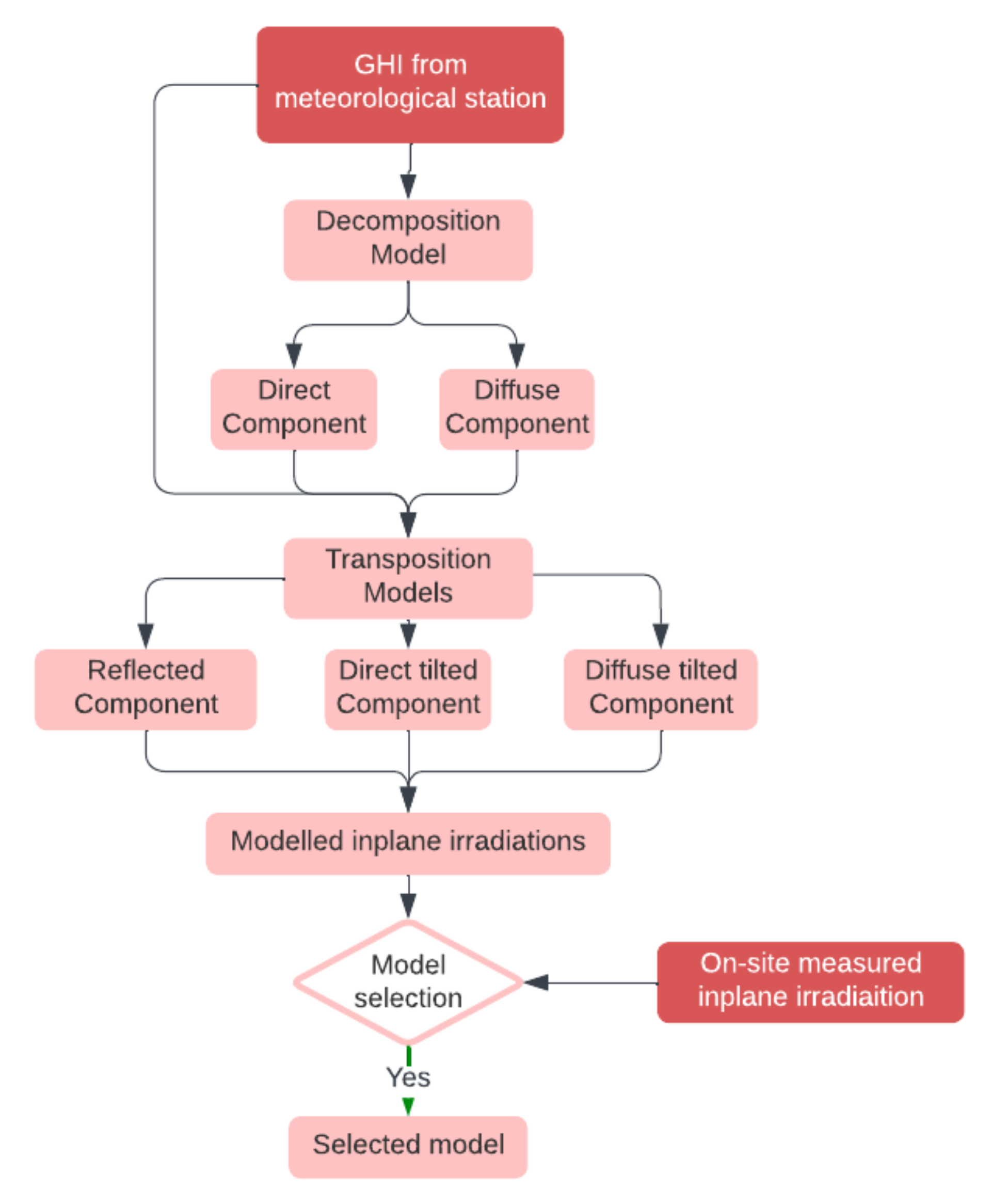
Venues selected for the analysis has different orientation and tilt angle as summarized in Table 2. Due to differences in orientation and tilt angle incident irradiation on module surfaces varies for each installation [35]. In-plane irradiation measurements are not present for the systems analyzed therefore in-plane irradiation is modelled by using global horizontal irradiation (GHI) data acquired from the government owned meteorological station located within 6 km. Modelled irradiation data is further compared with a recently installed on-site meteorological station data available from June 2021 until April 2022 and applicability of the data from the government-owned meteorological station is tested. A brief description of the pathway for modelling in-plane irradiation by using GHI data is summarized in Figure 1 below [36].

Initially, hourly GHI data gathered from meteorological station separated to its components as direct and diffuse radiation by using decomposition model proposed by Tapakis et al. This model is selected in this study due to the fact that it is proposed based on 10 years data collected from Athalassa’s Nicosia Cyprus actinometric station. Its accuracy is tested against 23 decomposition model and found to be the best performing model [37]. The governing model equations provided below.

$$k_d=0.9100+2.4993k_t-18.858k_t^2 When k_t<0.10$$

(1)

$$k_d=0.9605+0.4482k_t-2.0011k_{t }^2-1.5581k_t^3+2.0080k_t^4 when 0.10\le k_t\le 0.78$$

(2)

$$k_d=-2.4518+3.3014 k_t when 0.78\le k_t$$

(3)

where, $k_d$ is the ratio of diffuse irradiation $I_d$ to global horizontal irradiaiton $\left(GHI\right)$ $k_d=I_d /GHI$ and clearness index $k_t$, ratio of $GHI$ to extrateressial irradiaiton $(I_o$)$k_t=GHI/I_o$.

Equations (1)–(3) presented above evaluates diffuse component $I_d$ of the $GHI$ based on various clearness index $k_t$. Beam component I_b of $GHI$ is then simply the subtraction of $I_d$ from the $GHI$. $GHI$ is decomposed into its components as $I_b$ and $I_d$, then further used in transposition models for determining global tilted irradiance ($I_t$). I_t is a combination of of direct tilted ($I_{bt}$), diffuse tilted ($I_{dt}$) component and reflected component ($I_r$) given by the Equation (4) [36].

$$I_t=I_{dt}+I_{bt}+I_r$$

(4)

Transposition models have the same formula for $I_{bt}$ and I_r components_, only representation of $I_{dt}$ varies based on the model used. The models generally classified based on representation of $I_{dt}$ as isotropic and anisotropic. Isotropic models assume uniform distribution of $I_d$ over the sky dome. On the other hand, anisotropic models includes circumsolar irradiation, sky conditions and horizon brightening [36,38]. The governing components of $I_t$ is given below and summary of angle and their representative symbols is presented in

Table 4. Symbols and their angle representations.

Symbol	Angle
β	Tilte angle of PV modules
θ	Solar incidence angle
${\varphi }_z$	Solar zenith angle
γ	Surface azimuth angle
ω	Hour angle
δ	Declination angle
Φ	Local latitude

[38].

Direct tilted ($I_{bt}$) component

$$I_{bt}=R_b\times I_b$$

(5)

where $R_b$ is the ratio of beam radiation on tilted surface to that on a horizontal surface and represented by $R_b=cos\theta /cos{\varphi }_z$.

Reflected ($I_r$) component

The reflected component of irradiation on tilted surface is assumed to be isotropic and is dependent on GHI, albedo and tilt angle represented by the following equation [39,40,41,42]

$$I_r=GHI x \rho x \left(1-cos\beta \right)/2$$

(6)

where albedo, ($\rho$) is estimated as a constant 0.2 [38].

Diffuse tilted components ($I_{dt}$)

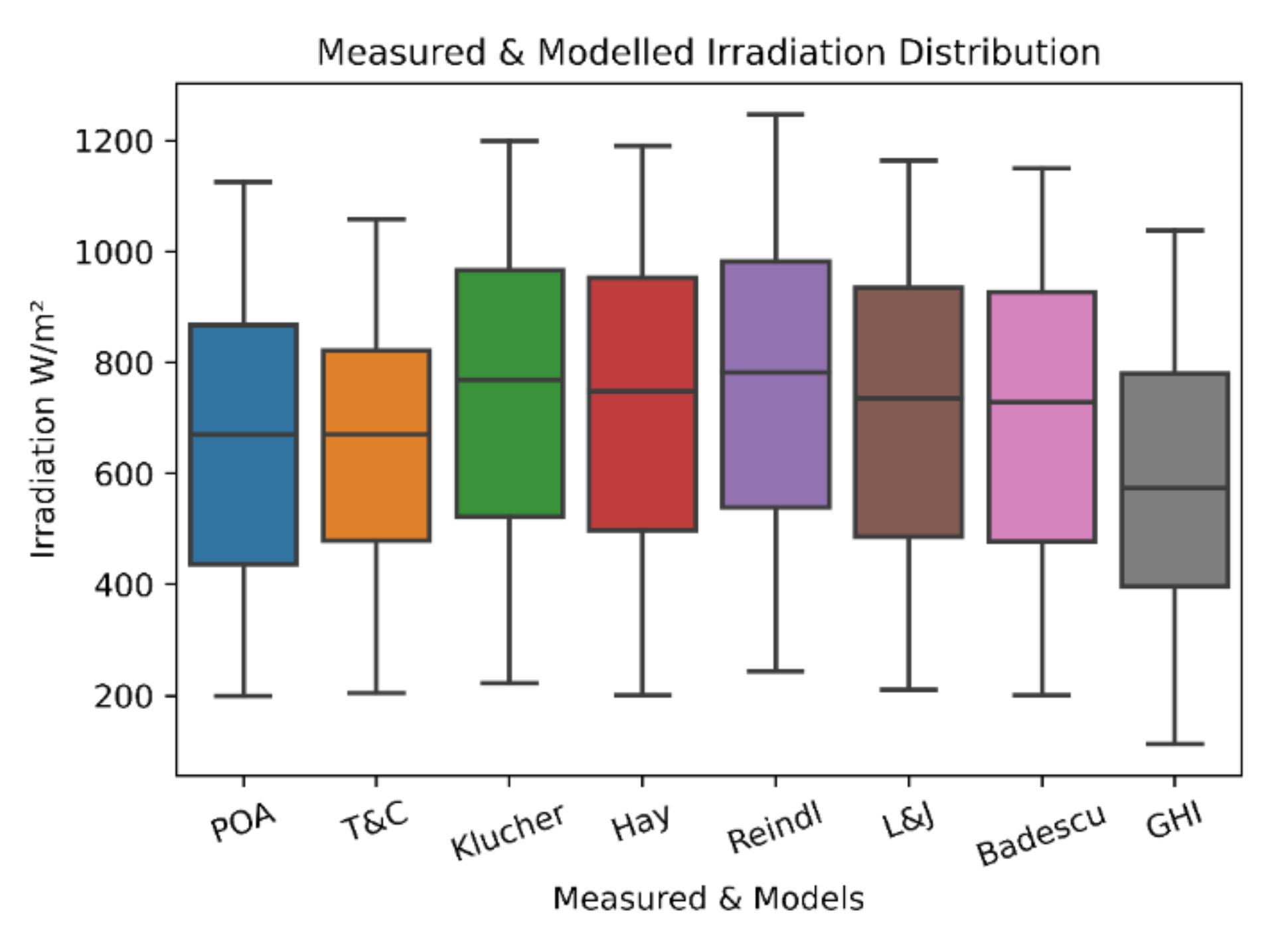
Two transposition models are proposed for the estimating the diffuse component specific to Cyprus [43,44] isotropic Badescu model [45] and anisotropic Temps-Coulson model [46]. In this analysis, four more models are used in addition to the two aforementioned models, namely isotropic Liu & Jordan [47] and the three anisotropic model Hay model [48], Klutcher model [49] and Reindl model [50]. The governing equations are provided below.

Temps-Coulson model

$$I{ }_{dt}=I_d\left(\frac{1+cos \beta }{2}\right)\left(1+co{s}^2\theta si{n}^3{\theta }_z\right) \left(1+si{n}^3\frac{\beta }{2}\right)$$

(7)

$$I{ }_r=I_H\times \rho \times \left|cos \gamma \right|\times \left(\frac{1-cos\beta }{2}\right)\times \left[1+si{n}^2\left(\frac{{\theta }_z}{2}\right)\right]$$

(8)

Liu & Jordan model

$$I{ }_{dt}=I_d\left(\frac{1+cos \beta }{2}\right)$$

(9)

Badescu model

$$I{ }_{dt}=I_d\frac{1}{4}\left(3+cos \left(2\beta \right)\right)$$

(10)

Hay model

$$I{ }_{dt}=I_d\left((\frac{B\times cos \theta }{G_{ext}cos{\theta }_z})+(1-\frac{B}{G_{ext}}) (\frac{1+cos \beta }{2})\right)$$

(11)

Klutcher model

$$I{ }_{dt}=I_d\left( \left(\frac{1+cos \left(\frac{\beta }{2}\right)}{2}\right)\times \left(1+f_{K}co{s}^2\theta co{s}^3{\theta }_z\right)\left(1+f_{K}si{n}^3\frac{\beta }{2}\right)\right)$$

(12)

where $f_K=1-{\left(D/G\right)}^2$ Reindl Model

$$I{ }_{d\beta }=I_d\left((\frac{B\times R_b}{G_{ext}})+(1-\frac{B}{G_{ext}}) (\frac{1+cos \beta }{2})\left(1+\sqrt{\frac{B}{G}}si{n}^3\frac{\beta }{2}\right)\right)$$

(13)

Diffuse tilted component is evaluated for each model by using the governing equations given above and combined with direct tilted component and reflected component to generate in-plane irradiation specific to each model. Furthermore, modelled in-plane irradiation is compared with the on-site data acquired by Sunny SensorBox (SMA Solar Technology AG, Niestetal, Germany). The performance of models is evaluated based on the root mean squared error (RMSE) and mean bias error (MBE) and R² value [51]. RMSE and MBE are computed as:

$$RMSE=\sqrt{\frac{1}{N}{{\displaystyle \sum }}_{i=1}^N{\left(X_e-X_m\right)}^2}$$

(14)

$$MBE=\frac{1}{N}{{\displaystyle \sum }}_{i=1}^N\left(X_e-X_m\right)$$

(15)

where, $X_e$ is the modelled irradiation and $X_m$ is the measured data.

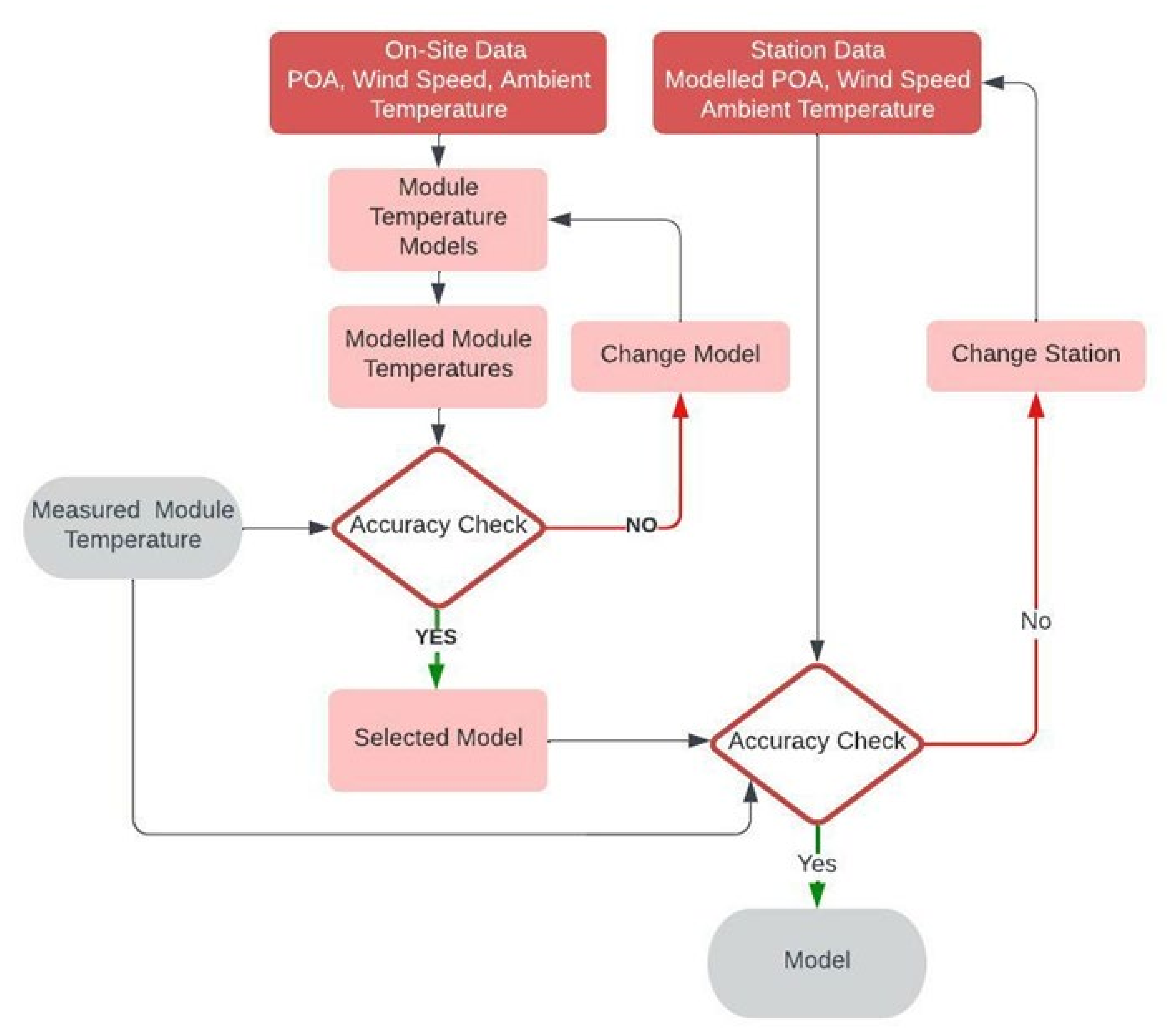
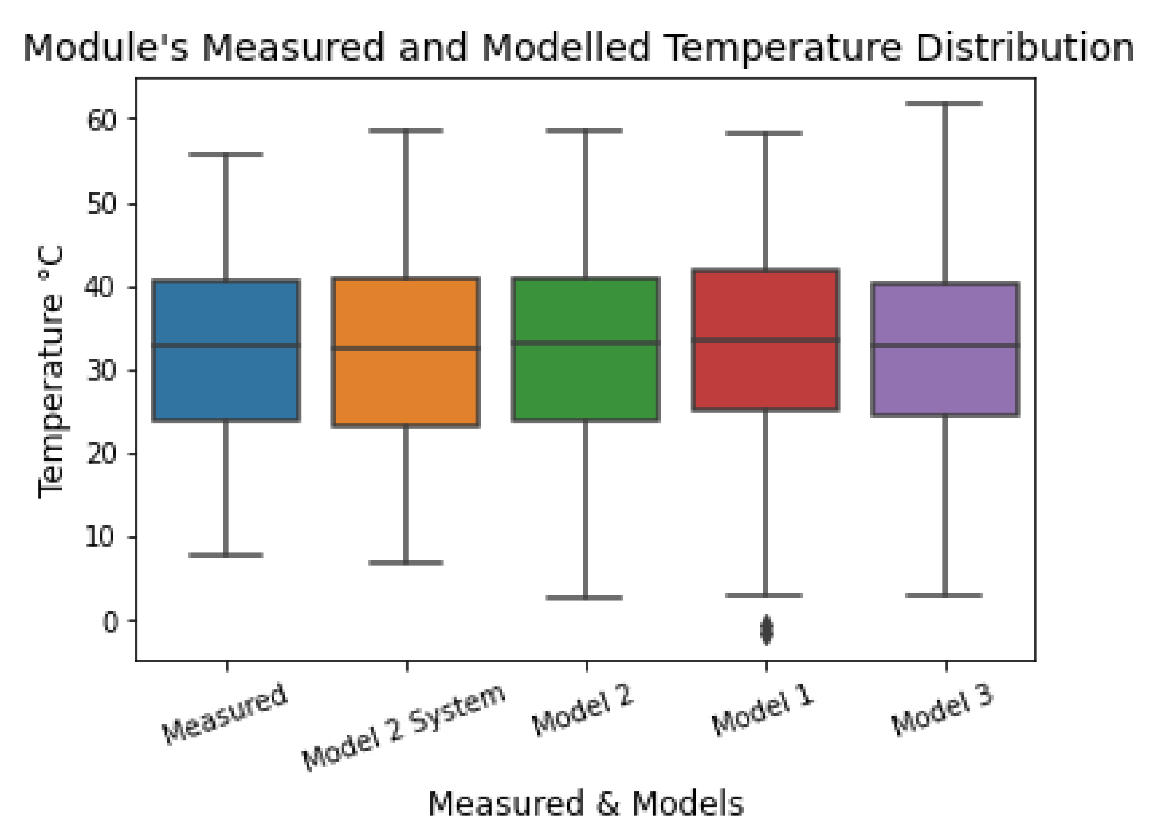
3.2. Modelling Module Temperature

Alongside the incident irradiation, power output of PV modules is also temperature dependent. Manufacturers generally provide the effect of temperature as %/°C on parameters such as Pmax, Voc and Isc. Depending on the selected performance metric module temperature or cell temperature needs to be modelled since direct measurements are not available [21,23]. The module temperature model selection procedure is provided in Figure 2.

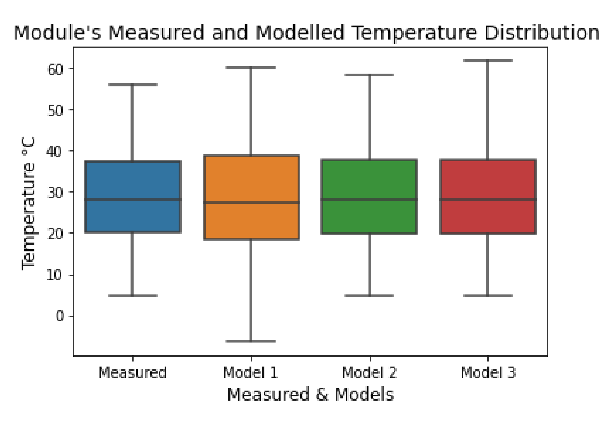
Various models are proposed in literature for determining module temperature $\left(T_m\right)$. Three arbitrarily selected model is provided below [52].

$$\mathrm{Model} 1: T_m=0.943T_a+0.028G-1.528v+4.3$$

(16)

$$\mathrm{Model} 2: T_m=T_a+0.0222I_t\left(1+0.009T_a\right)\left(1-0.063v\right)$$

(17)

$$\mathrm{Model} 3: T_m=T_a+\left(I_t/\left(25+6.8v\right)\right)$$

(18)

Initially wind speed (v), ambient temperature ($T_a$₎ and in plane irradiation $(I_t)$ data acquired from a nearby on-site station substituted into models provided above. The models result compared with on-site measured module temperature data. Performance of each model is evaluated based on RMSE Equation (14) and MBE Equation (15) as provided earlier. Among the tested models, the best performing model is selected and its accuracy further tested with wind speed and ambient temperature data acquired from the meteorological station coupled with modelled in-plane irradiation. The performance of selected model with meteorological data further tested on RMSE and MBE.

3.3. Filtering

The filtering step holds significance importance, specifically when modelling in plane irradiance from the global horizontal irradiation values acquired from the nearby station. Poor or variable solar resource conditions biasing data needs to be removed. Lindig et al., suggested the applied filter highly performance metric and statistical model dependent [53]. Furthermore, the filter choice is highly correlated with the outcome of the analysis, inappropriate filtering will yield wrong outcomes [6]; moreover, it provides depth to the analysis and may reveal practical issues such as inverter clipping [33]. IEC61724-3 suggests that the filtering criteria might change based on the local conditions and might yield better results.

In this study, two widely accepted filters are applied to the data; an irradiance low threshold filter of 200 W/m² is applied to in plane irradiation and high threshold is set to 1200 W/m². The low threshold filter is set to remove nighttime data and low irradiance periods. With the high threshold filter, measurement errors are omitted [22].

Another filter introduced for the dataset is the statistical filter. In-plane irradiation is modelled from GHI from a nearby station; therefore, some discrepancy might occur due to variation in irradiation. Therefore, a high filter (HF) and a variable low filter (LF) are set to maintain the power-irradiance relationship. Both filters are based on the measured irradiance and PV production correlation. The high filter is based on the fact that inverter production cannot be higher than maximum theoretical PV production.

For the low filter, the accuracy of the modelled monthly irradiation values is used as a guide. Generally, results suggested that from May to October, the in-plane irradiation has higher accuracy compared to rest of the year. Therefore, two different low filters arbitrarily set; LF_low is set for HF × 0.5 for May to October. LF_high is set for HF × 0.7 for November to April. LF_low also showed variability between venues in order to account for the variability in temperature variations and soiling effect.

$$\mathrm{HF}=\mathrm{module} \mathrm{rated} \mathrm{power} \times \mathrm{module} \mathrm{count} \times \mathrm{module} \mathrm{surface} \mathrm{area} \times \mathrm{PV} \mathrm{eff}. \mathrm{X} I_t$$

(19)

LF_low = HF × 0.5

(20)

LF_high = HF × 0.7

(21)

3.4. Metrics

Various performance metrics were utilized for determining PLR at system level [12,15,22]. Metrics used in this study are the performance ratio (PR), temperature corrected performance ratio (TCPR) and weather corrected performance ratio (NRELPR). Performance ratio PR is the most popular metric and is the ratio of the final energy yield of the system (kWh/kWp) to the reference yield (kWh/kW) described by the IEC 61724. In essence, it is an optimal performance parameter that represents the ability of a PV system to capture energy from the available in-plane irradiation under real life conditions and given by the following equation [28].

$$PR=\frac{{{\displaystyle \sum }}_{i}E{N}_{ac,i}}{{{\displaystyle \sum }}_i\left[P_{STC}\left(\frac{G_{POA,i}}{G_{STC}}\right)\right]}$$

(22)

where $E{N}_{ac,i}$ is the PV array output for a given period (day, month or year) $P_{STC}$ is the nominal power of the system, $G_{POA,i}$ is the inplane irradiation for a given period (day, month or year), $G_{STC}$ is the reference radiation 1 kW/m².

Performance ratio is prone to variations in ambient temperature. Power output of the PV modules are dependent on the ambient temperature based on their temperature coefficient. Dependency on temperature introduces high seasonal variations during the computation of performance ratio. The temperature-corrected performance ratio suggested by [28,30,31,34] introduces additional parameters that normalize the variations due to the operating temperature. The removal of seasonality due to the temperature variations favored the PRSTC for the degradation analysis [18]. The temperature-corrected performance ratio suggested by IEC 61724 is given by the following equation.

$$TCPR=\frac{{{\displaystyle \sum }}_{i}E{N}_{ac,i}}{{{\displaystyle \sum }}_i\left[P_{STC}\left(\frac{G_{POA,i}}{G_{STC}}\right)\left(1-\frac{\delta }{100}\left(T_{mod}-T_{ref}\right)\right)\right]}$$

(23)

$E{N}_{ac,i}$ is the PV array output for a given period (hour, day, month or year), $P_{STC}$ is the nominal power of the system, $G_{POA,i}$ is the in-plane irradiation for a given period (hour, day, month or year), $G_{STC}$ is the reference radiation 1 kW/m², $\delta$ is the PV module temperature coefficient of power (%/°C, negative in sign), $T_{mod}$: is the module temperature for a given period (hour, day, month or year), $T_{ref}$: is the reference module temperature STC, 25 °C.

Another methodology is developed by National Renewable Energy Laboratory. It is aimed to have a better representation of a weather corrected PR. This methodology incorporates the weather-related effects including ambient temperature, wind and irradiation.

The Weather corrected PR is estimated by the following equation [27,34].

$$NRELPR=\frac{{{\displaystyle \sum }}_{i}E{N}_{ac,i}}{{{\displaystyle \sum }}_i\left[P_{STC}\left(\frac{G_{POA,i}}{G_{STC}}\right)\left(1-\frac{\delta }{100}\left(T_{cell\_type\_avg}-T_{cel{l}_i}\right)\right)\right]}$$

(24)

The main difference between weather corrected performance ratio and IEC 61724 is the accommodation of normalization parameters. The formula suggested by IEC724 was based on the module temperatures while formula suggested by NREL uses the cell temperature equation as follow $T_{cell}=T_m+\frac{G_{POA}}{G_{STC}}\times \Delta Tcnd$ where $T_m$ is the module back temperature and can be evaluated by $T_m=G_{poa}\times e^{\left(a+b\times WS\right)}+T_a$ where $e^{\left(a+b\times WS\right)}$ conduction/convection heat transfer coefficient °C.m²/kW. WS is the wind m/s. The coefficients (a, b and ΔTcnd) are the empirical coefficients and recommended by King, Boyson, and Kratochvill (2004) [54] for a Glass/cell/polymer sheet module type in a free ventilation installation is −2,81, −0.0455 and 3, respectively. Average irradiance weighted cell temperature is calculated from the following equation.

$$T_{cell\_type\_avg}={\displaystyle \sum }\left(G_{POA\_type\_j}\times T_{cell\_typ\_j}\right)/{\displaystyle \sum }\left(G_{poa\_type\_J}\right)$$

(25)

$T_{cell\_type\_avg}$ (Average irradiance-weighted cell temperature from one year of weather data using the project weather file, $T_{cell\_typ\_j}$ = calculated cell operating temperature for each hour, $G_{POA\_type\_j}$ = POA irradiance for each hour, J is each hour of the year (8760 h total).

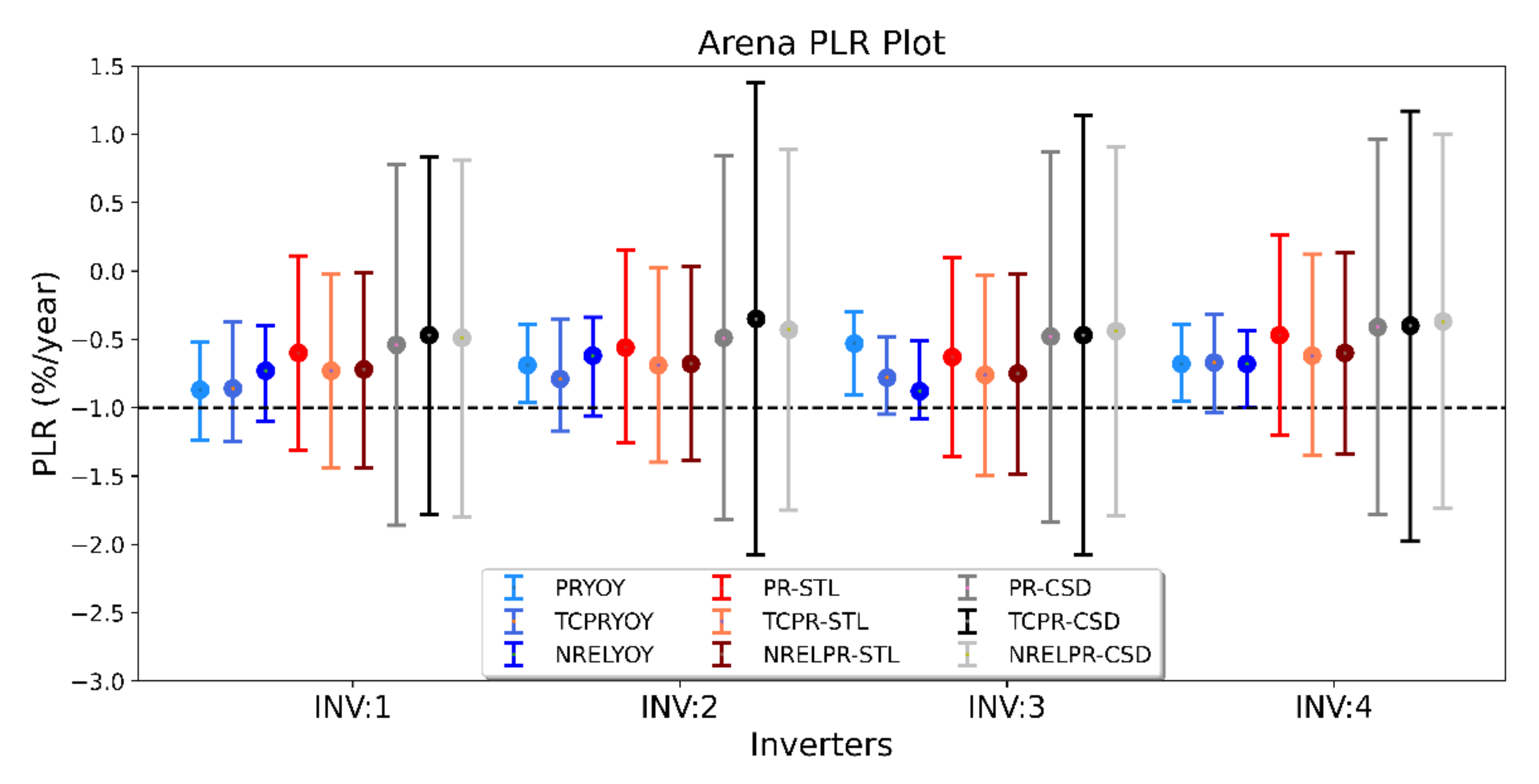
3.5. Statistical Approach

Various statistical methods are proposed for the PLR calculations. In this study, three statistical methods are coupled with the performance metrics for determining PLR, namely seasonal trend decomposition by LOESS (STL), Classical Seasonal Decomposition (CSD), and Year on year (YOY) analysis.

The CSD method introduced in 1920s forms the basis of time series decomposition techniques. The main objective of decomposition models is to remove the seasonality from the data such that the trend can be seen more clearly. Even some of the normalized metrics used in this study accounts the variability of temperature, however, the soiling effect perseveres. Classical decomposition models represented below in Equation (26).

$$Y=T_t+S_t+e_t$$

(26)

where $Y$ is the time series, $T_t$ is the trend, $S_t$ is the seasonal and $e_t$ is the residual component. The trend is obtained from the original data with a centered 12 month moving average. The seasonality component is obtained by subtracting the trend from the original data. Each month is averaged across the year; the combined seasonal component and the trend are extracted from the original time series to find the residual components [17,53]. The seasonal component is assumed to be constant over the years and due to the twelve months centered moving average; the first and last six months are not included in computation [53,55].

STL is a robust algorithm used for decomposition of time series. Similarly to CSD, STL also separates time series to three components: seasonal, trend and reminder. The seasonal component is a recurring pattern present in data. Once determined, it is removed from the time series data to eliminate the seasonal component. Dissimilar to the centered moving average for extracting trend in CSD method, the trend is extracted from locally weighted polynomial fitting in STL [17,53,56]. The remainder of the component is obtained by subtracting the trend and the seasonal component. STL method is more prone to outliers, outages and missing data due to its locally formed trend.

STL and CSD analysis are conducted by using the python package ‘statmodels’ to analyze monthly data of metrics [57]. Annual degradation rates were evaluated by applying the linear regression on the trend of both CSD and STL.

$$y=ax+b$$

(27)

Once the slope (a) and the intercept (b) are extracted yearly relative PLR is calculated by the following equation $PLR=\frac{12a}{b}$. and the uncertainty is of PLR is calculated by the following equation [53].

$$u_{plr}=\sqrt{\left({\left(\frac{12}{b}\right)}^2\times u_a^2+{\left(\frac{-12a}{b^2}\right)}^2\times u_b^2\right)}$$

(28)

where a and b are the fitting coefficients of the linear regression, $u_{a,b}^2$ the variances of fitting coefficients and $u_{plr}$ the standard deviation of PLR.

Lastly, YoY method proposed by Hasselbrink et al., as a comparative method different than the statistical analysis. This was further developed by Jordan et al., for the assessment of daily metrics. YoY method evaluates the rate of change for two points in subsequent years based on the duration taken into account (monthly, weekly and daily). This procedure is repeated for every point of throughout the monitoring period. Furthermore, a distribution of rate of changes are generated and median of this distribution, representing the performance loss rate of the system [33,58]. Median value provides more robust analysis due to the reduction in impact of outliers over the mean value [15].

4. Results and Discussions

4.1. Modelled Irradiation

Boxplot of modelled in-plane irradiation, measured in-plane irradiation and GHI is given in Figure 3. Performance analysis of the modelled tilted irradiation is summarized in

Table 5. MBE RMSE and R² of the models.

Model	MBE	RMSE	R2
TC	−50.70	123.09	0.84
HA	−58.23	123.64	0.84
BA	−45.00	114.42	0.86
LJ	−46.35	116.92	0.85
KL	−73.80	130.90	0.82
RE	−94.42	144.01	0.79

. For the period 2021 June to 2022 April, results suggested that Badescu model has the lowest MBE and RMSE and also has the highest R². In contrast, Reindl model has the highest MBE and RMSE and also has the lowest R². Accuracy of the other models are ranked between these values. Therefore, Badescu model is used to generate in-plane irradiation in this study. On the other hand, findings of Tapakis et al., suggested Temps and Coulson model is the most suitable model among tested 10 models in Cyprus. However, this analysis is limited and only covers the period of two months February and March [44]. When results of the analysis further investigated in monthly basis, the outcome suggests that Temps and Coulson model is the most accurate model in February, March and April in line with the findings of Tapakis et al. [44].

In addition, monthly findings presented below suggests that the accuracy of model is higher for the duration of 6 months covering period from April until the end of October as shown in

Table 6. Monthly performance of Badescu model.

Months	MBE	RMSE	R2
Jun.	−73.26	104.19	0.89
Jul.	−73.26	96.33	0.90
Aug.	−55.34	71.70	0.95
Sep.	−32.45	102.31	0.89
Oct.	−25.30	106.77	0.88
Nov.	−0.79	120.12	0.80
Dec.	−5.55	136.51	0.75
Jan.	−15.22	143.36	0.74
Feb.	−23.36	135.99	0.78
Mar.	−42.66	147.86	0.78
Apr.	−58.00	89.39	0.92

. This is probably due to the clearer sky conditions for this period.

4.2. Modelled Temperature

On-site measurements including ambient temperature, wind speed, and measured irradiation is used for the assessment of models for predicting the module temperatures. Boxplot of measured and modelled module temperatures are provided in Figure 4.

Performance analysis of the models for modelling module temperature is summarized in

Table 7. Model Module temperature performances.

Models	MBE	RMSE	R2
Model 1	0.546	3.408	0.903
Model 2	0.026	0.774	0.995
Model 3	−0.031	1.164	0.989

. Based on on-site measured data, Model 2 proposed by Servant et al., has the lowest MBE and lowest RMSE and the highest R² among the tested models and owing to its higher accuracy it selected for modelling the module temperature by using parameters acquired from the closest meteorological station [59].

The accuracy of selected model is further tested in order to clarify the influence of distance on module temperature between venues. For this, modelled in-plane irradiation, wind speed and ambient temperature data from the meteorological station used with selected model along with other models to assess their performances.

The box plots of measured and modelled module temperature results are shown Figure 5. Moreover, the performance analysis of the module temperature models generated by using meteorological station data is provided in

Table 8. Performance of models with meteorological data.

Models	MBE	RMSE	R2
Model 1	−1.025	4.930	0.778
Model 2	−0.227	3.910	0.864
Model 3	−0.159	4.390	0.824

.

Variability in model performances was expected due to the fact that in-plane irradiation, wind speed and ambient temperature might change between two measurement sites. Model 2 still generates the lowest MBE, RMSE and highest R² value among the tested models. On the other hand, it has higher MBE, RMSE and lower R².

4.3. Filter

The evolution of performance ratio plots as the filters applied is presented in Figure 6. Figure 6a represents the PR values without any filter. In Figure 6b, low threshold filter of 200 W and high threshold filter of 1200 W is applied to PR values. Before introducing variable LF, arbitrarily introduced fixed filter of LF (HF × 0.5) and HF is coupled with 200 W and 1200 W applied to the data throughout the year. Suspicious and unrepresentative data significantly reduced, as shown in Figure 6c. With applied filters, downward trend in PR values is observed specially in winters. This might be due to possible variations in weather conditions between meteorological station and the installation site. Introducing variable LF as explained in Section 3 removed the downward trend as shown in Figure 6d.

4.4. Performance Loss Rates

The systems investigated between 2016 and 2020 covered a period of 4 years, for the venues Arena, Stonite and Arazi. Almost 1 MWp of polycrystalline PV modules wired to total number of 42 SMA 25,000 TL inverters are investigated. In Arazi, the installation two of the inverters, INV:6 and INV:22, are not considered in this study due to failure to generate any power over a year. The annual averaged daily PR for venues Arena, Arazi and Stonite is 0.79, 0.76 and 0.74, respectively. Our findings are in agreement with the findings of Makrides et al., in Arena installation [31]. While two venues have relatively lower PRs. Randomly selected daily PR plots of different inverters, INV 23 from Arazi, INV:1 from Arena and INV:2 from Stonite are presented in Figure 7, respectively. PR plot for Stonite installation differs from the Arazi and Arena PR plots as the modules undergo heavy soiling, occuring from June to October repeatedly over the years. In 2016, a reduction trend of PR started in June by the end of July PR amount to 0.55 and by mid-August lowest PR is registered as 0.43. Similar patterns were observed over the years. The lowest PR was registered as 0.29 in October 2017. Similar excessive reduction in PR values was observed for Arena installation, though only in 2017. Gradual reduction in PR values observed in 2017, starting in summer until mid-October. The lowest daily PR recorded as 0.49 on 15th October and registered PR values was around 0.5 for a week. Further though the end of October PR values increased back to 0.7, indicating possible cleaning of the modules. During the rest of the year, daily PR remained above 0.60. Dissimilar from previous two venues, the Arazi daily PR plot remained above 0.6 throughout the analyzed years. Considering installation angles of the venues, drops in PR plots may link to the soiling of PV modules. Occasional soiling in Arena installation is observed in the summer of 2017, and severe soiling in Stonite installation throughout the monitoring period due to their lower tilt angle. On the other hand, limited reduction in PR is observed in Arazi installation with a higher installation angle. Severe drop in daily PR plot of Arena during the summer of 2017 may be linked to a rainless period or inadequate rainfall and lack of maintenance during this period. Moreover, severe losses in daily PR values for Stonite installation also may be linked to excess soiling caused by a nearby operating brick factory. The brick factory uses clay, fine grains used for brick production and coal ash from the chimney of furnaces contributing to reductions in PR values.

Figure 8 represents PLRs of Arena inverters estimated by various metrics and statistical approaches. In general, YOY approach generated higher PLRs compared to CSD and STL methods. The uncertainty of YOY approach is the lowest. The average PLR of Arena installation from different methods is determined in two ways by grouping degradation rates based on normalization metric and statistical approaches. The PLR of Arena plant based on statistical approaches YOY, STL and CSD are −0.73, −0.65 and −0.44%/year, respectively. The average PLR based on normalized metrics namely PR, TCPR and NRELPR and variable are −0.57, −0.63 and −0.62%/year, respectively. Based on YOY, the averaged PLR of Inverter 1 is −0.82%/year, highest among all the inverters. From STL INV:3 has the highest PLR with 0.71%/year. Both methods suggest INV:4 has the lowest PLR.

The CSD Statistical approach is not presented for the analysis of later two venue Arazi and Stonite due to high uncertainties and occasional positive degradation results in the Stonite installation. Outliers have big impact on CSD method [52], even with the diligent filtering, some of the outlier PR data persists. Moreover, fast improvement and deterioration cycles due to cleaning and soiling might cause underestimating PLR.

Figure 9 represents PLRs of Stonite inverters estimated by various metrics and statistical approaches for Stonite installation. In general, STL approach generated the higher PLRs than YOY methods. The uncertainty of methods of YOY approach is lower than STL method. The average PLR of Stonite installation is separated into two groups based on normalization metric and statistical approaches. The PLR of Stonite plant, based on statistical approaches YOY and STL, are −2.65 and −2.91%/year, respectively. On the other hand, the average PLR based on normalized metrics PR, TCPR and NRELPR are −2.71, −2.84 and −2.78%/year, respectively.

The highest PLRs among all venues were observed in Stonite. PLRs of INV:2 is the highest regardless of normalization metric and statistical approach used. PLRs of INV:1 is the lowest when STL method is considered. On the other hand, PLRs of INV:6 is the lowest with the YOY approach. The highest annual PLRs of Temperature corrected metrics NRELPR and TCPR combined with STL method is above 4%. PLRs of aforementioned metrics with YOY approach is −3.64% and −3.85%/year, respectively. Specific to this location, the YOY approach generated higher variances compared to STL model, specially INV:6 has shown the highest variances.

Figure 10 represents PLR of Arazi inverters estimated by various metrics and statistical approaches for Arazi installation. In general, YOY approach generated the higher PLRs than STL methods. The uncertainty of methods of STL method is lower than YOY approach. The average PLR of Arena installation is separated into two groups based on normalization metric and statistical approaches. The PLR of Arena plant based on statistical approaches YOY and STL (average PLR of PR, TCPR and NRELPR metrics) are −1.20% and −0.69%/year, respectively. On the other hand, the average PLR based on normalized metrics PR, TCPR and NRELPR are −0.92%, −0.97% and −0.95%/year, respectively.

PLRs of INV:4 is the highest based on both the YOY approach and the STL method. On the other hand, lowest PLRs varied and YOY results suggested PLRs of INV:1 is the lowest and PLRs of INV:10 is the lowest when the STL method is considered. The normalization metric PR has generated the highest PLRs compared to temperature corrected metrics regardless of statistical approach. Averaged PLRs of metric PR YOY is 77% higher than the PR STL. The difference between the two statistical approaches is the highest among the analyzed venues.

Results suggested that statistical approach generate higher PLR differences compared to metrics therefore results of each metric averaged based on the statistical approach and represented in

Table 9. Representing average PLRs of each venue with average confidence intervals.

Venues	PLR YOY	YOY CIL	YOY CIH	PLR STL	STL CIL	STL CIH
ARAZI	−1.2	−0.89	−1.51	−0.69	−0.49	−0.89
ARENA	−0.73	−0.4	−1.07	−0.65	0.02	−1.37
STONITE	−2.65	−2.02	−3.07	−2.91	−2.01	−3.21

. The highest PLR occurred in STONITE installation as expected hotspots are observed on PV modules due to excessive soiling. Thee PLR of Arazi installation was the second highest. Average percentage difference between the YOY approach and the STL method is 10% for the PLR of Arena and Stonite installation. However, in the ARAZI installation, the percentage difference between the YOY and the STL method exceeded 70%. The Arazi installation is a ground mount system, based on the site observations; growing grasses shades PV modules, high bird dropping rate, arbitrarily cleaning PV modules might cause nonlinearity in data and influencing the metric utilized. Ultimately shifting the median hence, the PLR. Frick et al., have investigated the degradation rate of multiple multi-c-Si systems, each having a total capacity of around one kW_p, for over 12 years in Cyprus. Results suggested annual degradation rate varied between 0.2% and 1.2%. For some systems, the YOY approach resulted in wider variations in degradation estimations in agreement with the current study. These variations in YOY are attributed to the presence of hotspots and nonlinearly deteriorating PV modules [15].

Lastly, Arena has the lowest PLR among analyzed venues. Despite its low installation angle, both YOY approach and STL method resulted PLR less than 1%/year. This is probably related to minimum soiling effect as it is constructed over asphalt carpark and also good ventilation due to high-level structure.

Averaging normalized metrics regardless of statistical approach yield similar PLR as shown in

Table 10. Illustrating avarage PLRs of each venue based on normalization metrics.

Venues	PR	NRELPR	TCPR
ARAZI	0.92	−0.97	−0.95
ARENA	0.57	−0.63	−0.62
STONITE	2.71	−2.84	−2.78

. Moreover, it is revealed that temperature corrected metrics yields higher PLR values. Relative to PLRs determined by PR metric, temperature corrected metrics increased PLRs of Arena, Arazi and Stonite by 9.65%, 4.35% and 3.68%, respectively. Furthermore, a negative correlation was observed between PLRs and temperature corrected metrics. As the annual PLR rate increased, the percentage increase rate reduced. A similar comparative analysis between PR and TCPR conducted by Phinikarides et al., reported a percentage increase in TCPR relative to PR, as much as 65% [14].

Phinikarides et al., compared 5 years degradation rates of various PV technologies in Cyprus by using PR and Temp corrected PR coupled with statistical analysis STL Findings of this study suggests a degradation rate of −1.12%/year and −0.94%/year for TCPR STL and PR-STL, respectively [14]. These results are in-line with the outcome of the current study, only with higher PR-STL values −0.70% and −0.57% in Arazi and Arena, respectively, but higher in Stonite, −2.75%. On the other hand, the TCPR STL results of our study −0.68% for Arazi, −0.70% for Arena and −3.06% for Stonite.

5. Conclusions

This study presents PLR analysis of 1045 kW_p PV plant, composed of three different venues within two km. The performance of the three venues, namely Arena, Arazi and Stonite located in Nicosia, the capital of Cyprus, is investigated during the operation period from 2016 to 2020. Through the study, in-plane irradiation and module temperature are modelled by using data acquired from the nearest meteorological station located within 6 km and model accuracies are justified with an on-site weather station. For modelling in-plane irradiation from GHI, the simple isotropic Badescu model is found to be the most accurate among tested 6 models with the lowest MBE and RMSE. Furthermore, we found that model proposed by Servant et al., had a better representation of measured module temperature among the other two models [59]. Modelled data and PV productions are then used to evaluate three most commonly used performance metrics; PR, TCPR, NRELPR. Furthermore, performance metrics combined with statistical methods CSD, STL and YOY are used to analyze the PLR. The mean PLRs of each venue varied based on the statistical approach and metric used. The outcome of this study suggested variations in PLR are more dependent on statistical approach compared to performance metrics. When the YOY approach combined with performance metrics, PLRs of Arazi, Arena and Stonite are −1.2/%year, −0.73/%year and −2.65/%year, respectively. With the STL method, PLRs of Arazi, Arena and Stonite are −0.69/%year, −0.65/%year and −2.91/%year, respectively. In general, PLRs of the venues are highly varied over the operation period. Variability in PLRs of analyzed system proves that PLRs are site specific. Moreover, the maintenance and cleaning frequency should be adapted with the site conditions. Better maintenance and cleaning schedule will not only improve the yield of the system, but it will improve the system’s lifespan.

References

1. IEA. Electricity Market Report-January 2022; IEA: Paris, France, 2022; Available online: https://www.iea.org/reports/electricity-market-report-january-2022 (accessed on 20 June 2022).
2. Solargis, Solar Radiation Map of Cyprus. Available online: https://solargis.com/maps-and-gis-data/download/cyprus (accessed on 20 June 2022).
3. Ren21. Renewables 2021 Global Status Report, Renewable Energy Policy Network for the 21st Century; Ren21: Paris, France, 2020. [Google Scholar]
4. Renewable Energy Board–January 2022, Nicosia, North Cyprus. Available online: https://yek.gov.ct.tr/ (accessed on 31 January 2022).
5. Lindig, S.; Theristis, M.; Moser, D. Best practices for photovoltaic performance loss rate calculations. Prog. Energy 2022, 4, 022003. [Google Scholar] [CrossRef]
6. Lindig, S.; Kaaya, I.; Weis, K.-A.; Moser, D.; Topic, M. Review of Statistical and Analytical Degradation Models for Photovoltaic Modules and Systems as Well as Related Improvements. IEEE J. Photovolt. 2018, 11, 1312–1318. [Google Scholar] [CrossRef]
7. Schlothauer, J.; Jungwirth, S.; Köhl, M.; Röder, B. Degradation of the encapsulant polymer in outdoor weathered photovoltaic modules: Spatially resolved inspection of EVA ageing by fluorescence and correlation to electroluminescence. Sol. Energy Mater. Sol. Cells 2012, 102, 75–85. [Google Scholar] [CrossRef]
8. Czanderna, A.W.; Pern, F.J. Encapsulation of PV modules using ethylene vinyl acetate copolymer as a pottant: A critical review. Sol. Energy Mater. Sol. Cells 1996, 43, 101–181. [Google Scholar] [CrossRef]
9. Kaplani, E. Degradation effects in sc-si PV modules subjected to natural and induced ageing after several years of field operation. J. Eng. Sci. Technol. Rev. 2012, 5, 18–23. [Google Scholar] [CrossRef]
10. Dhimish, M.; Alrashidi, A. Photovoltaic Degradation Rate Affected by Different Weather Conditions: A Case Study Based on PV Systems in the UK and Australia. Electronics 2020, 9, 650. [Google Scholar] [CrossRef] [Green Version]
11. Shin, W.; Ko, S.; Song, H.; Ju, Y.; Hwang, H.; Kang, G. Origin of Bypass Diode Fault in c-Si Photovoltaic Modules: Leakage Current under High Surrounding Temperature. Energies 2018, 11, 2416. [Google Scholar] [CrossRef] [Green Version]
12. Jordan, D.C.; Silverman, T.J.; Sekulic, B.; Kurtz, S.R. PV degradation curves: Non-linearities and failure modes. Prog. Photovolt. Res. Appl. 2016, 25, 583–591. [Google Scholar] [CrossRef] [Green Version]
13. Jordan, D.C.; Silverman, T.J.; Wohlgemuth, J.H.; Kurtz, S.R.; VanSant, K.T. Photovoltaic failure and degradation modes. Prog. Photovolt. Res. Appl. 2017, 25, 318–326. [Google Scholar] [CrossRef]
14. Phinikarides, A.; Makrides, G.; Georghiou, G. Comparison of analysis methods for the calculation of degradation rates of different photovoltaic systems. In Proceedings of the 28th European Photovoltaic Solar Energy Conference and Exhibition, Paris, France, 30 September–4 October 2013; pp. 3973–3976. [Google Scholar]
15. Frick, A.; Makrides, G.; Schubert, M.; Schlecht, M.; Georghiou, G. Degradation Rate Location Dependency of Photovoltaic Systems. Energies 2020, 13, 6751. [Google Scholar] [CrossRef]
16. Paudyal, B.; Bolen, M.; Fregosi, D. PV Plant Performance Loss Rate Assessment: Significance of Data Filtering and Aggregation. In Proceedings of the 2019 IEEE 46th Photovoltaic Specialists Conference (PVSC), Chicago, IL, USA, 16–21 June 2019; pp. 866–869. [Google Scholar] [CrossRef]
17. Jordan, D.C.; Kurtz, S.R. Analytical improvements in PV degradation rate determination. In Proceedings of the 35th IEEE Photovoltaic Specialists Conference, Honolulu, HI, USA, 20–25 June 2010; pp. 2688–2693. [Google Scholar] [CrossRef] [Green Version]
18. Khan, F.; Kim, J.H. Performance Degradation Analysis of c-Si PV Modules Mounted on a Concrete Slab under Hot-Humid Conditions Using Electroluminescence Scanning Technique for Potential Utilization in Future Solar Roadways. Materials 2019, 12, 4047. [Google Scholar] [CrossRef] [Green Version]
19. Kyranaki, N.; Smith, A.; Yendall, K.; Hutt, D.; Whalley, D.; Gottschalg, R.; Betts, T. Damp-heat induced degradation in photovoltaic modules manufactured with passivated emitter and rear contact solar cells. Prog. Photovolt. Res. Appl. 2022, 1–11. [Google Scholar] [CrossRef]
20. Wu, Z.; Lv, S.; Song, H.; Yun, M. Statistical Modeling of UV-Induced PV Module Power Degradation Based on Acceleration Tests. IEEE J. Photovolt. 2019, 10, 144–149. [Google Scholar] [CrossRef]
21. Quansah, D.; Adaramola, M.; Takyi, G. Degradation and longevity of solar photovoltaic modules—An analysis of recent field studies in Ghana. Energy Sci. Eng. 2020, 8, 2116–2128. [Google Scholar] [CrossRef] [Green Version]
22. Ingenhoven, P.; Belluardo, G.; Makrides, G.; Georghiou, G.E.; Rodden, P.; Frearson, L.; Herteleer, B.; Bertani, D.; Mose, D. Analysis of Photovoltaic Performance Loss Rates of Six Module Types in Five Geographical Locations. IEEE J. Photovolt. 2019, 9, 1091–1096. [Google Scholar] [CrossRef]
23. Gopi, A.; Sudhakar, K.; Keng, N.; Krishnan, A. Comparison of normal and weather corrected performance ratio of photovoltaic solar plants in hot and cold climates. Energy Sustain. Dev. 2021, 65, 53–62. [Google Scholar] [CrossRef]
24. Ameur, A.; Berrada, A.; Bouaichi, A.; Loudiyi, K. Long-term performance and degradation analysis of different PV modules under temperate climate. Renew. Energy 2022, 188, 37–51. [Google Scholar] [CrossRef]
25. Silvestre, S.; Tahri, A.; Tahri, F.; Benlebna, S.; Chouder, A. Evaluation of the performance and degradation of crystalline silicon-based photovoltaic modules in the Saharan environment. Energy 2018, 152, 57–63. [Google Scholar] [CrossRef]
26. Malvoni, M.; Kumar, N.M.; Chopra, S.S.; Hatziargyriou, N. Performance and degradation assessment of large-scale grid-connected solar photovoltaic power plant in tropical semi-arid environment of India. Sol. Energy 2020, 203, 101–113. [Google Scholar] [CrossRef]
27. Carigiet, F.; Brabec, C.; Baumgartner, F. Long-term power degradation analysis of crystalline silicon PV modules using indoor and outdoor measurement techniques. Renew. Sustain. Energy Rev. 2021, 144, 111005. [Google Scholar] [CrossRef]
28. Hassan Daher, D.; Gaillard, L.; Ménézo, C. Experimental assessment of long-term performance degradation for a PV power plant operating in a desert maritime climate. Renew. Energy 2022, 187, 44–55. [Google Scholar] [CrossRef]
29. Jordan, D.C.; Smith, R.M.; Osterwald, C.R.; Gelak, E.; Kurtz, S.R. Outdoor PV Degradation Comparison. In Proceedings of the 35th IEEE Photovoltaic Specialists Conference, Honolulu, HI, USA, 20–25 June 2010; pp. 2694–2697. [Google Scholar] [CrossRef] [Green Version]
30. Sorloaica-Hickman, N.; Davis, K.; Leyte-Vidal, A.; Kurtz, S.; Jordan, D. Comparative study of the performance of field-aged photovoltaic modules located in a hot and humid environment. In Proceedings of the 38th IEEE Photovoltaic Specialists Conference, Austin, TX, USA, 3–8 June 2012; pp. 2376–2381. [Google Scholar] [CrossRef]
31. Makrides, G.; Zinsser, B.; Georghiou, G.E.; Schubert, M.; Werner, J.H. Degradation of different photovoltaic technologies under field conditions. In Proceedings of the 35th IEEE Photovoltaic Specialists Conference, Honolulu, HI, USA, 20–25 June 2010; pp. 2332–2337. [Google Scholar] [CrossRef]
32. Kunaifi, K.; Reinders, A.; Lindig, S.; Jaeger, M.; Moser, D. Operational performance and degradation of PV systems consisting of six technologies in three climates. Appl. Sci. 2020, 10, 5412. [Google Scholar] [CrossRef]
33. Jordan, D.C.; Deceglie, M.G.; Kurtz, S.R. PV degradation methodology comparison—A basis for a standard. In Proceedings of the IEEE 43rd Photovoltaic Specialists Conference (PVSC), Portland, OR, USA, 5–10 June 2016; pp. 273–278. [Google Scholar] [CrossRef]
34. Jordan, D.C.; Deline, C.; Kurtz, S.R.; Kimball, G.M.; Anderson, M. Robust PV Degradation Methodology and Application. IEEE J. Photovolt. 2018, 8, 525–531. [Google Scholar] [CrossRef]
35. Obiwulu, A.; Erusiafe, N.; Olopade, M.; Nwokolo, S. Modeling and estimation of the optimal tilt angle, maximum incident solar radiation, and global radiation index of the photovoltaic system. Heliyon 2022, 8, 09598. [Google Scholar] [CrossRef] [PubMed]
36. Lave, M.; Hayes, W.; Pohl, A.; Hansen, C.W. Evaluation of Global Horizontal Irradiance to Plane-of-Array Irradiance Models at Locations Across the United States. IEEE J. Photovolt. 2015, 5, 597–606. [Google Scholar] [CrossRef]
37. Tapakis, R.; Michaelides, S.; Charalambides, A.G. Computations of diffuse fraction of global irradiance: Part 1–Analytical modelling. Sol. Energy 2016, 139, 711–722. [Google Scholar] [CrossRef]
38. Maleki, S.M.; Hizam, H.; Gomes, C. Estimation of Hourly, Daily and Monthly Global Solar Radiation on Inclined Surfaces: Models Re-Visited. Energies 2017, 10, 134. [Google Scholar] [CrossRef] [Green Version]
39. Demain, M.; Journee, C. Evaluation of different models to estimate the global solar radiation on inclined surfaces. Renew. Energy 2013, 50, 710–721. [Google Scholar] [CrossRef]
40. Padovan, A.; Del Col, D. Measurement and modeling of solar irradiance components on horizontal and tilted planes. Sol. Energy 2010, 84, 2068–2084. [Google Scholar] [CrossRef]
41. Evseev, E.G.; Kudish, A.I. The assessment of different models to predict the global solar radiation on a surface tilted to the south. Sol. Energy 2009, 83, 377–388. [Google Scholar] [CrossRef]
42. Gueymard, C.A. Direct and indirect uncertainties in the prediction of tilted irradiance for solar engineering applications. Sol. Energy 2009, 83, 432–444. [Google Scholar] [CrossRef]
43. Kavas, G. Estimation of diffuse solar irradiation and its effects on pv power plant production at METU NCC. Master’s Thesis, Middle East Technical University, Northern Cyprus Campus, Kalkanlı, Northern Cyprus, 2019. [Google Scholar]
44. Tapakis, R.; Charalambides, A.G. Performance evaluation of a photovoltaic park in Cyprus using irradiance sensors. J. Power Technol. 2014, 94, 296–305. [Google Scholar]
45. Badescu, V. 3D isotropic approximation for solar diffuse irradiance on tilted surfaces. Renew. Energy 2002, 26, 221–233. [Google Scholar] [CrossRef]
46. Temps, R.C.; Coulson, K.L. Solar radiation incident upon slopes of different orientations. Sol. Energy 1977, 19, 179–184. [Google Scholar] [CrossRef]
47. Liu, B.; Jordan, R.C. The interrelationship and characteristic distribution of direct, diffuse and total solar radiation. Sol. Energy 1960, 4, 1–19. [Google Scholar] [CrossRef]
48. Hay, J.E. Calculation of monthly mean solar radiation for horizontal and inclined surfaces. Sol. Energy 1979, 23, 301–307. [Google Scholar] [CrossRef]
49. Klucher, T.M. Evaluation of models to predict insolation on tilted surfaces. Sol. Energy 1979, 23, 111–114. [Google Scholar] [CrossRef]
50. Reindl, D.T.; Beckman, W.A.; Duffie, J.A. Evaluation of hourly tilted surface radiation models. Sol. Energy 1990, 45, 9–17. [Google Scholar] [CrossRef]
51. Fan, Y.; Wang, Z.; Wang, J.; Cai, L.; Zhao, B.; Zhou, M.; Li, Q. Evaluation of 12 Transposition Models Using Observations of Solar Radiation and Power Generation. IEEE J. Photovolt. 2022, 12, 444–452. [Google Scholar] [CrossRef]
52. Santiago, I.; Trillo-Montero, D.; Moreno-Garcia, I.M.; Pallarés-López, V.; Luna-Rodríguez, J.J. Modeling of photovoltaic cell temperature losses: A review and a practice case in South Spain. Renew. Sustain. Energy Rev. 2018, 90, 70–89. [Google Scholar] [CrossRef]
53. Lindig, S.; Ascencio-Vásquez, J.; Leloux, J.; Moser, D.; Reinders, A. Performance Analysis and Degradation of a Large Fleet of PV Systems. IEEE J. Photovolt. 2021, 11, 1312–1318. [Google Scholar] [CrossRef]
54. King, D.L.; Boyson, W.E.; Kratochvill, J.A. SANDIA REPORT SAND 2004-3535 Unlimited Release Printed December 2004 Photovoltaic Array Performance Model. 2005. Available online: https://www.semanticscholar.org/paper/SANDIA-REPORT-SAND-2004-3535-Unlimited-Release-2004-King-Boyson/923f653e82c599633bb755a093aaddf8912bbbd9 (accessed on 20 June 2022).
55. Tabatabaei, S.A.; Formolo, D.; Treur, J. Analysis of performance degradation of domestic monocrystalline photovoltaic systems for a real-world case. Energy Procedia 2017, 128, 121–129. [Google Scholar] [CrossRef]
56. Luo, W.; Isukapalli, S.N.; Vinayagam, L.; Ting, S.A.; Pravettoni, M.; Reindl, T.; Kumar, A. Performance loss rates of floating photovoltaic installations in the tropics. Sol. Energy 2021, 219, 58–64. [Google Scholar] [CrossRef]
57. Seabold, S.; Perktold, J. Statsmodels: Econometric and Statistical Modeling with Python. In Proceedings of the 9th Python in Science Conference, Austin, TX, USA, 28 June–2 July 2010. [Google Scholar]
58. Hasselbrink, E.; Anderson, M.; Defreitas, Z.; Mikofski, M.; Shen, Y.C.; Caldwell, S.; Terao, A.; Kavulak, D.; Campeau, Z.; DeGraaff, D. Validation of the PVLife model using 3 million module-years of live site data. In Proceedings of the IEEE 39th Photovoltaic Specialists Conference (PVSC), Tampa, FL, USA, 16–21 June 2013; pp. 7–12. [Google Scholar] [CrossRef]
59. Servant, J. Calculation of cell temperature for photovoltaic modules from climatic data. In Proceedings of the 9th Biennal Congress of the International Sol Energy Society-Intersol, Montreal, QC, Canada, 23–29 June 1985; pp. 1640–1643. [Google Scholar]
Figure 1. Illustrating steps for modelling in-plane irradiaiton.
Sustainability 14 09084 g001
Figure 2. Demonstrating module temperature.
Sustainability 14 09084 g002
Figure 3. Box plot of modeled and measured tilted irradiaition.
Sustainability 14 09084 g003
Figure 4. Box plot of modelled and measured module temperatures (on-site data).
Sustainability 14 09084 g004
Figure 5. Box plot of measured and modelled module temperature (meteorological station data).
Sustainability 14 09084 g005
Figure 6. Evolution of PR plots with applied filters. (a) No filter, (b) Threshold filter (c) Fixed LF filter, (d) Variable LF filter.
Sustainability 14 09084 g006
Figure 7. Representing PR of an inverter from each venue.
Sustainability 14 09084 g007
Figure 8. PLRs of Arena.
Sustainability 14 09084 g008
Figure 9. PLRs of Stonite.
Sustainability 14 09084 g009
Figure 10. PLRs of ARAZI.
Sustainability 14 09084 g010