1. Introduction
Spatial data are multidimensional and include the location information of certain events or objects and their non-spatial attributes. Ideally, the relationship between locations and attributes should be investigated using complete data for every location in the study region. In practice, however, such spatially continuous and complete data are difficult, if not impossible, to collect due to the time and cost required [
1]. Missing and incomplete observations are common in most real-world datasets, and thus, the use of reliable and accurate imputation methods has become crucial to complement them [
2].
In recent decades, there have been numerous studies on the estimation of missing values in spatial data. The relevant literature can be divided into two broad groups: (1) empirical studies that focus on utilizing spatial statistics and other imputation methods and (2) more methodological works that aim to identify the most accurate and reliable imputation method through comparative analysis. In the former, spatial interpolation techniques, such as inverse distance weighting (IDW) and kriging, have been commonly used to estimate unobserved values, especially when spatial autocorrelation is present in the data. However, machine learning techniques, such as neural networks and random forests, have become popular in recent years because of their successful application in various domains [
3,
4,
5,
6,
7,
8].
Although machine learning has shown its potential and usefulness in various academic and industrial fields, it is still essential to understand its advantages and limitations as a spatial imputation tool compared to the existing interpolation methods [
9]. While previous studies have demonstrated that machine learning techniques, such as neural networks and random forests, can estimate the missing values more accurately than the traditional distance-based functions, the results varied depending on the training data size and the characteristics of the target variable to be imputed. Considering that much of the existing literature is in the field of environmental sciences, the application of machine learning techniques to socio-spatial data still needs further evaluation.
To complement this limitation in the current literature, this work evaluates the strengths and drawbacks of machine learning as an imputation method in the context of social and spatial studies. More specifically, we aim to address the following two research questions:
Are the state-of-the-art machine learning models capable of estimating missing values in the spatial data representing complex urban phenomena, such as house prices?
If so, are they more accurate than the conventional spatial interpolation approaches?
To answer these questions, we employ two of the most popular techniques, namely neural networks and random forests, to estimate the prices of the houses for which no transactions are recorded in the real estate transaction data of Seoul, South Korea. The results are then compared to those from IDW and kriging using a set of accuracy metrics, such as the root mean square error (RMSE) and mean absolute error (MAE). The findings from this empirical analysis will help us better understand the capabilities of machine learning in social sciences and urban analytics, especially for imputing missing values in massive spatial data with socioeconomic attributes.
2. Past Studies
In statistics, imputation refers to the process of replacing missing values with substituted ones using ancillary data [
10]. Proper use of the imputation can minimize any bias caused by missing values and ensure the efficiency of data processing and analysis. Single imputation methods, such as hot-deck, mean substitution, and regression, have been widely used because of their simplicity in solving problems. However, multiple imputations, which provide an ensemble of the uncertainty of errors by performing a set of single imputations, have also been increasingly adopted in recent years.
In the fields of geography, geology, and environmental sciences, interpolation methods such as IDW and kriging have been commonly used to predict unobserved values in datasets [
11]. Past studies show that a simple distance-based function, such as IDW, works reasonably well in certain settings (e.g., the case of bathymetry in [
12]), but kriging is often considered a more robust tool as it can take auxiliary variables into account. For example, Wu and Li [
13] argued that the temperature could be more accurately interpolated when the variable ‘altitude’ was included in the model, along with latitude and longitude. Bhattacharjee et al. [
14] also demonstrated that a cokriging model incorporating a range of weather variables into the temperature prediction could produce more precise estimations than a model relying only on distances.
While these interpolation methods have usually been applied to environmental variables, such as precipitation, temperature, and humidity, some efforts have been made to use IDW and kriging for the imputation of socioeconomic data with location information [
15,
16]. Montero and Larraz [
17] attempted to estimate the prices of commercial properties in Toledo using IDW, kriging, and cokriging and concluded that cokriging performed better than the others when auxiliary variables were chosen appropriately. Similarly, Kuntz and Helbich [
18] found that cokriging predicted the house prices in Vienna more precisely than its other variants. These results seem to be supported by the cases of other cities and countries [
19,
20].
Meanwhile, more recent studies focus on how the development of machine learning can enhance the accuracy of imputation accuracy and replace the existing interpolation methods. Because machine learning techniques, such as neural networks and random forests, can handle the complexity and nonlinearity of real-world datasets, they can be advantageous in predicting missing and unobserved values [
21]. For the imputation of environmental variables, several studies have been conducted to assess the performance of machine learning, and promising results have been reported over the past decade [
3,
9]. In particular, random forests yielded a significant improvement in various empirical cases, suggesting that they can be a reliable alternative to conventional statistical approaches.
The efforts were not limited to the environmental studies. Pérez-Rave and colleagues [
22], for example, proposed an integrated approach of the hedonic price regressions model and machine learning and demonstrated its advantages in predicting real estate data. Čeh et al. [
23] also compared random forests and the hedonic model based on multiple regression to predict apartment prices. They found that the random forest models could detect and predict data variability more accurately than the traditional approaches.
Nonetheless, it is still difficult to generalize that machine learning outperforms interpolation methods in predicting missing values. While many studies illustrate the successful applications of such state-of-the-art techniques, their effectiveness and efficiency for a particular problem depend on the size and nature of the data at hand [
24]. In the case of spatial data representing socioeconomic attributes, such as house prices, more empirical analyses should be conducted to verify the relative strengths and drawbacks of machine learning [
2]. To this end, this study applies neural networks and random forests, currently the two most popular machine learning techniques, to estimate unobserved values in real estate transaction data and compares the results to those from the interpolation methods.
3. Data and Methods
3.1. Data
This study uses the real estate transaction data for Seoul, South Korea. It is a public dataset provided by the Ministry of Land, Infrastructure, and Transport (MOLIT) and contains all the sales and rental transaction records from 2006. We utilized only the sales records between 2015 and 2019 as input data because the rental prices are determined by various external factors and may not represent the actual value of the properties.
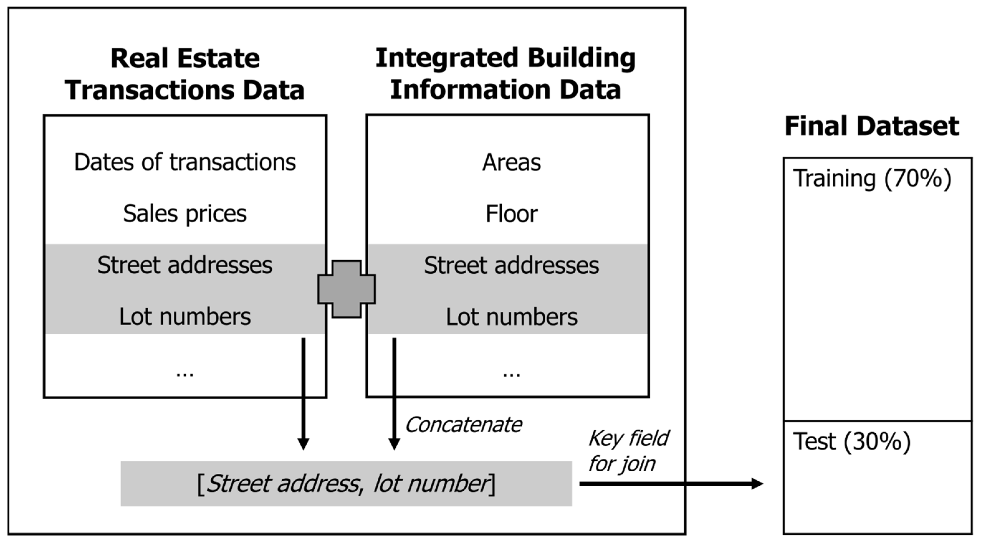
The real estate transactions data consist of several transaction-related variables, ranging from the dates of the transactions to the sales (or rental) prices. However, they do not include cadastral information, such as the year of construction, land and building areas, and the number of floors. MOLIT provides such information as a separate dataset called the integrated building information data. Therefore, we merged the two datasets manually to prepare the training and test datasets, as illustrated in
Figure 1.
The real estate transactions data have two fields for location information, namely lot numbers and street addresses (or sometimes called road name addresses). The integrated building information data have the same fields as well, but some adjustments are required to match the location information of the two datasets. Therefore, we concatenated the two fields to form a single field of [street address, lot number] and used it as a key field during the joining process. Any transactions not matched to the integrated building information data were removed from the final dataset.
It may be worth noting that the sales transactions were made multiple times for some properties during the study period. Consequently, there were duplicate points in the final dataset, each representing one transaction. Although we tried to minimize data loss during the merging process, some transaction records were dropped because of incomplete or inaccurate address information.
The final dataset consisted of 287,034 observations with 16 variables. We randomly selected approximately 70% of these, or 200,924 observations, to train the prediction models; we tested the accuracy of each model using the remaining 30% (i.e., 86,110 observations).
Table 1 lists the names, descriptions, and types of the variables. The sales price per unit was the target variable to be imputed, and all the other variables were used as predictor variables. Note that the interpolation methods adopted in the present study cannot consider auxiliary variables other than the
x and
y coordinates; therefore, the estimation is based only on the distances between the properties.
3.2. Methods
In this study, we examine the accuracy and efficiency of four methods—neural networks, random forests, IDW, and kriging—as imputation tools for spatial data representing socioeconomic attributes, specifically house prices.
A neural network model comprises one input layer and one output layer, and there can be multiple hidden layers between the two. The input layer takes raw data values and feeds them into one or more hidden layers in the middle of the model. The data values are weighted and summed at each hidden layer and then passed through an activation function to the next hidden or output layer [
25]. The number of hidden layers in a neural network model is directly related to its ability to handle nonlinearity in the data. As the number of hidden layers increases, a more complex relationship between the input and output variables can be addressed; however, the risk of overfitting simultaneously escalates [
26].
The learning process of a neural network involves backpropagation, which propagates errors in the reverse direction from the output layer to the input layer and updates the weights in each layer. While this is a crucial step for ensuring the accuracy and reliability of the model [
27,
28], backpropagation in a large network with many hidden layers and nodes can be computationally expensive. Therefore, for successful and effective use of neural networks, it is essential to choose the appropriate number of hidden layers and nodes, along with other hyperparameters, through iterative refinement.
Random forest is one of the most popular ensemble techniques; it forms multiple decision trees using subsets of the input data, trains them through random bootstrapping, and aggregates the trees into a final model [
29]. In a random forest model, one predictor variable is randomly selected at each branch of decision trees, and such randomness minimizes bias and reduces the correlation between the trees [
29]. Previous studies found that random forests are robust to missing observations and outliers [
30] and can produce more accurate and reliable results than traditional decision trees.
One practical drawback of random forests is that they cannot visualize the results in an intuitive graph form, as in the case of decision trees. If the significance of predictor variables is required to simplify and optimize the model, it should be estimated separately. In this study, we estimate the relative importance of variables by calculating the out-of-bag (OOB) errors for decision trees with
n-1 variables. If the error changes marginally when a specific variable is removed, the variable can be eliminated from the model, as it has only a slight impact on the result [
31]. To obtain the best possible prediction results from random forests, the predictor variables should be chosen based on the OOB errors, and the other hyperparameters, such as the number of trees, should be carefully tuned [
32].
IDW is the simplest spatial interpolation method and has been used for several decades [
11]. For each location to be imputed, it computes a weighted average of all the observed values, where the weight of observations is determined based on their distance to the location of interest,
s0 [
33]. The equation for IDW can be formulated as
where
refers to the estimated value at point
s0, and
is the observed value at point
si.
represents the weight applied to
and is calculated as
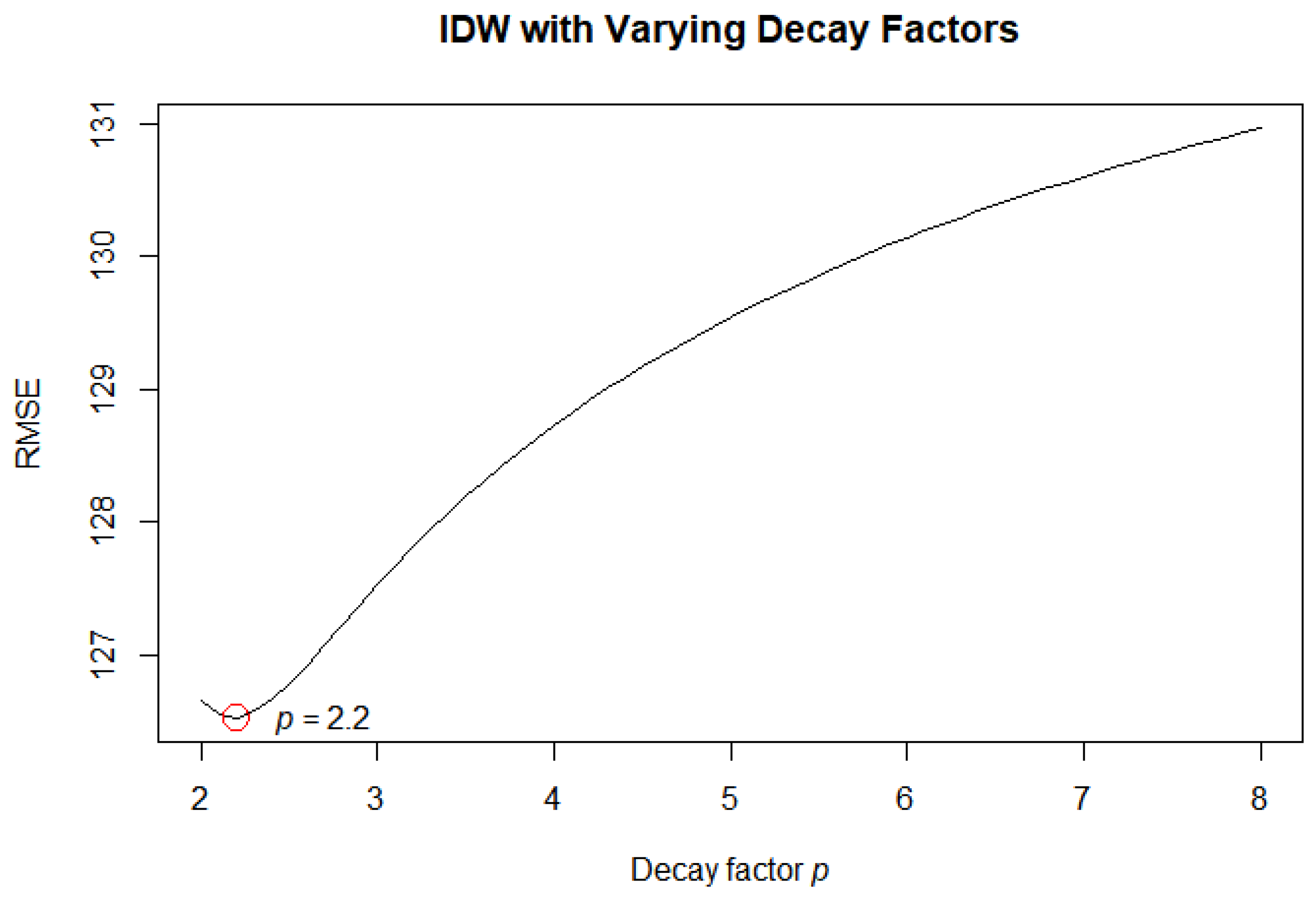
The distance decay parameter, p, defines how rapidly the influence of distant points decreases. As p increases, the weights for points distant from s0 become significantly smaller than those for the close points. It is set to 2 by default in most computer software; however, because the choice of p is crucial for the performance of IDW, it is desirable to test several candidates and choose the one that produces the most accurate and explainable results.
Kriging is a weighted linear regression that utilizes observed values from neighboring locations to predict missing or unknown values [
34]. Kriging has many variants, including simple, ordinary, and universal kriging. The most appropriate variant depends on the variable of interest. If the mean of the target variable is constant in the study area and its exact value is known, simple kriging can minimize the prediction errors. However, if the mean of the target variable is unknown, or if it is non-stationary, the use of either ordinary or universal kriging is ideal [
35,
36,
37].
Cokriging refers to a family of methods that incorporate associated variables into the kriging models. Cokriging has the same variants as kriging—simple, ordinary, and universal—and it tends to perform better than its univariate counterparts, as briefly discussed in
Section 2 (see, for example, [
14]). However, in this study, none of the ancillary variables available (i.e., those presented in
Table 1) was sufficiently correlated with the target variable. The strongest correlation of 0.285 was observed between the land areas and sales prices per unit, but it was not strong enough to expect any improvements from the use of cokriging [
38]. Furthermore, there was no apparent trend in the mean of the target variable; so, we chose ordinary kriging as the most suitable method for the provided data. The semivariogram parameters, including nugget, sill, and range, were chosen through iterations to obtain the best fitting model for ordinary kriging.
4. Model Optimization
To obtain the most accurate predictions from each method presented in the previous section, it is crucial to optimize the model hyperparameters [
39]. The hyperparameters were iteratively changed in this study, and the accuracies were assessed through cross-validation. To avoid overfitting, we divided all of the data into training and test sets for model building and validation, respectively. For IDW and kriging, however, there were no learning processes involved; therefore, these methods were directly applied to the test set. The root mean square error (RMSE) was employed as the primary metric during the optimization process, and the hyperparameters that minimized the RMSE were selected for each model.
The neural network models were constructed by adjusting the number of hidden layers and the number of nodes in the hidden layers. The batch size, indicating the total number of training data in a single batch, was fixed at 64, and the epochs for the model optimization were set at 150, considering the size of the training set. The activation and loss functions were set to a rectified linear unit (ReLU) and mean square error (MSE), respectively.
Table 2 indicates that the RMSE decreases in general as the number of hidden layers and nodes increases. However, it also suggests that the RMSE would increase if the scale of the network exceeded a certain point. Therefore, in this study, we chose a model with four hidden layers, a maximum of 256 nodes, and a minimum of 128 nodes as the optimal neural network model, as it yielded the lowest RMSE.
The random forest models were built by varying the numbers of trees and predictor variables for node branching. The number of trees increased by 50 from 50 to 200. For each decision tree, the number of predictor variables was set to 4, 8, and 16, making 12 models in total. The cross-validation results show that the error tends to decrease as we increase the number of trees and predictor variables. In
Table 3, the model with 200 trees and 16 predictor variables has the lowest RMSE; so, we chose it as the optimal model for the random forest.
In IDW, because the model estimation depends only on the distance decay parameter
p, we examined the accuracy by gradually increasing it from 2 to 8 by 0.1. The results are presented in
Figure 2, where the RMSE is the lowest at
p = 2.2; therefore, it was chosen as the optimal parameter for IDW.
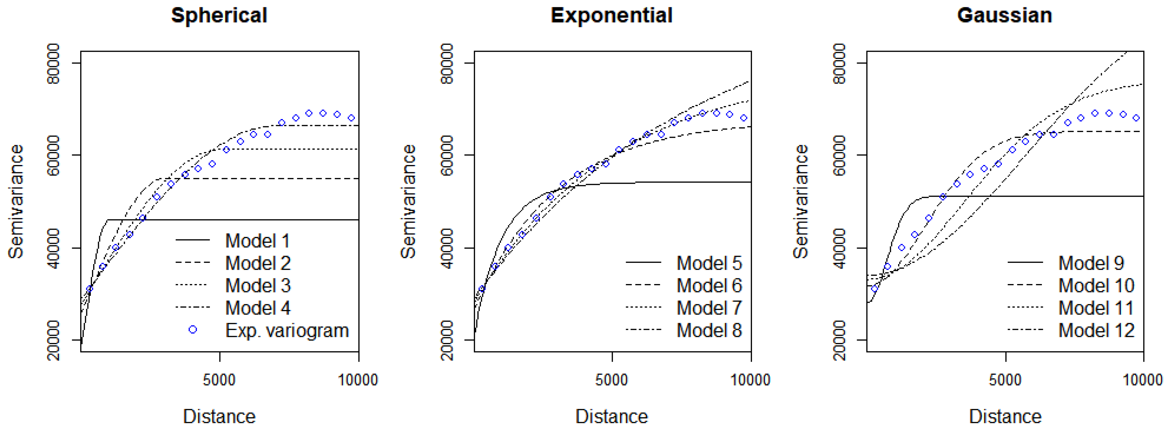
In ordinary kriging, the models were constructed by varying the semivariogram parameters, namely the model type, nugget, sill, and range (
Figure 3). As shown in
Table 4, we tested the spherical, exponential, and Gaussian models to fit the semivariogram. For each model, we used four different range values (i.e., 1000, 3000, 5000, and 7000) with default nugget and sill values. Overall, the spherical function provided more accurate results, and the RMSE seemed to decrease as the range decreased (
Table 4).
5. Results
The models selected from the previous section were applied to the test datasets. For comparison,
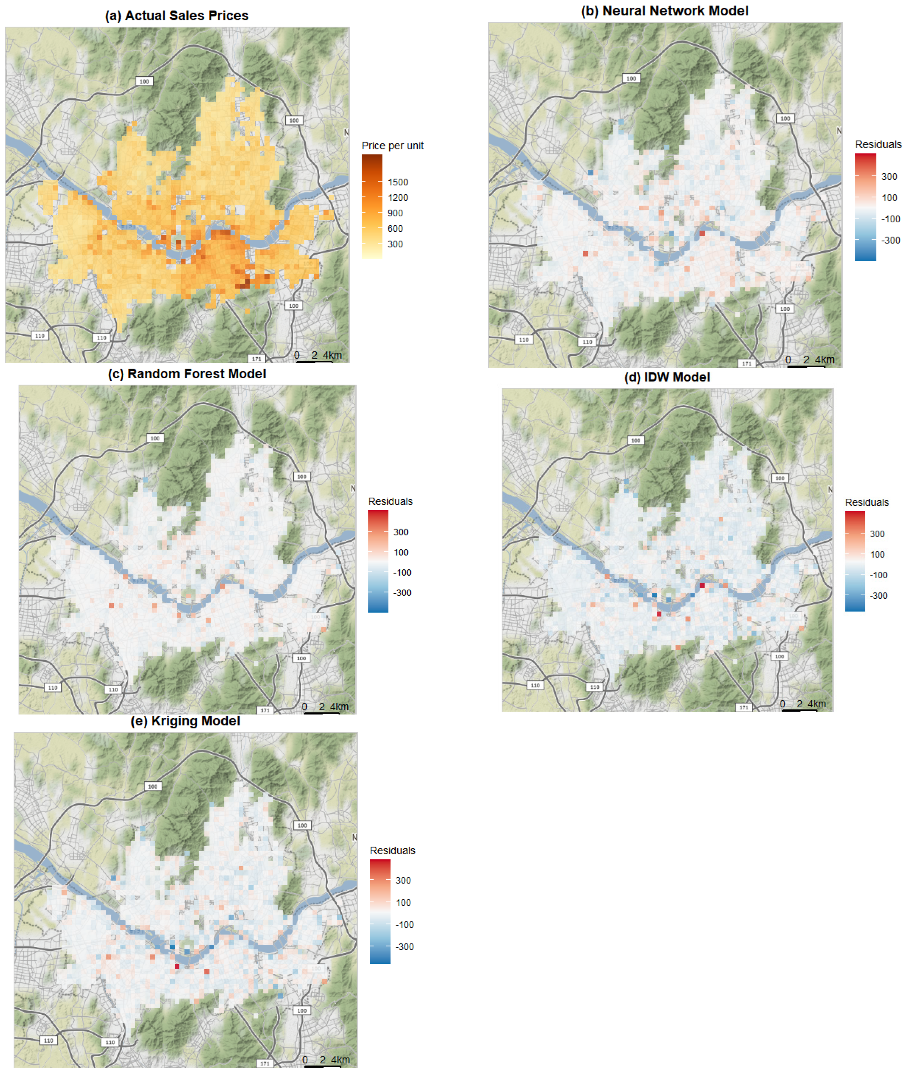
Figure 4 shows the distribution of the actual house prices and the residuals (i.e., the difference between the actual and the predicted prices) from each method. Due to the volume of the data and the presence of many duplicate points, the results could not be visualized using raw points. Instead, we created grids and calculated the average values for each grid. In
Figure 4a, the grids with high average sales prices are marked in dark red, whereas those with low prices are marked in light yellow. The red and blue colors in
Figure 4b–e indicate the positive and negative residuals, respectively.
Figure 4a shows that the high sales prices are clustered around the central and bottom parts of the city, as well as along the Han River. The residuals from the neural network model tend to be small and positive, but there are some large discrepancies between the actual and the predicted values around where the expensive properties are located (
Figure 4b). The random forest model has a similar visual impression (
Figure 4c), and it is difficult to conclude which model is better from these maps.
In contrast, it is relatively apparent that IDW and kriging produced higher residuals in some parts of the city.
Figure 4d implies that both over- and underestimation of house prices have occurred. There are both negative and positive residuals, and some of those along the river are considerable in size. The pattern in
Figure 4e is similar; however, the residuals tend to be smaller than those from IDW, and there appears to be no clustering of large residuals in the central part of the city. Overall, these results imply that IDW and kriging are less reliable for predicting house prices than the machine learning methods. House prices are determined by a complex interplay of various geographic, demographic, and social factors, and thus, the conventional spatial interpolation methods that rely on a distance-based function may not be sufficient to establish an accurate model.
In addition to these visual comparisons, we adopted several accuracy metrics, including the mean absolute error (MAE), mean absolute percentage error (MAPE), mean absolute scale error (MASE), and RMSE, for a more comprehensive evaluation.
The MAE is the mean of the absolute error between the actual and predicted values. Because the MAE represents the absolute value of the error, a smaller MAE value implies a higher accuracy of the model. As it does not involve multiplication, it is less affected by outliers than the RMSE. The MAPE is defined as the error divided by the actual, observed value. As the actual value is used as a denominator, it should be non-zero. If the actual value is less than one, and if it gets closer to zero, the MAPE approaches infinity. The last metric in this study, MASE, on the other hand, divides the error by the normal variation range to determine whether the error occurs outside of the variation range. This metric is particularly useful when comparing variables with different variances.
Table 5 presents the calculated accuracy metrics. All metrics indicate that the random forest model is the most accurate, followed by the neural network model. The accuracies of IDW and Kriging were found to be the lowest. These findings indicate that the machine learning techniques could be superior to the distance-based interpolation methods for predicting house prices.
This result can be attributed to the number of data points used in this study. In ordinary kriging, although the imputation process is simple when the amount of data is small, the calculation time increases significantly when a large amount of data is available, making it difficult to fully utilize the given data [
40]. On the other hand, most machine learning techniques are designed to work with large data, and the accuracy of the model improves as the volume of the data increases in general. The data in this study amounted to almost 300,000 transactions, resulting in a higher accuracy with the machine learning techniques than the spatial interpolation counterparts.
Among the machine learning techniques, the random forest model yielded higher accuracy than the neural network model. One reason behind this is that the real estate transaction data are in a tabular form. When tabular data are used in neural networks, the structure of the model can become highly dimensional or overparameterized, resulting in overfitting issues during the analysis process [
41,
42,
43]. Conversely, the tree-based ensemble model can be more efficient for high-dimensional tabular data [
44], and it has the advantage of preventing overfitting by considering the balance between biases and variances [
29]. For this reason, the random forest model might perform better than the neural network for predicting house prices in this study.
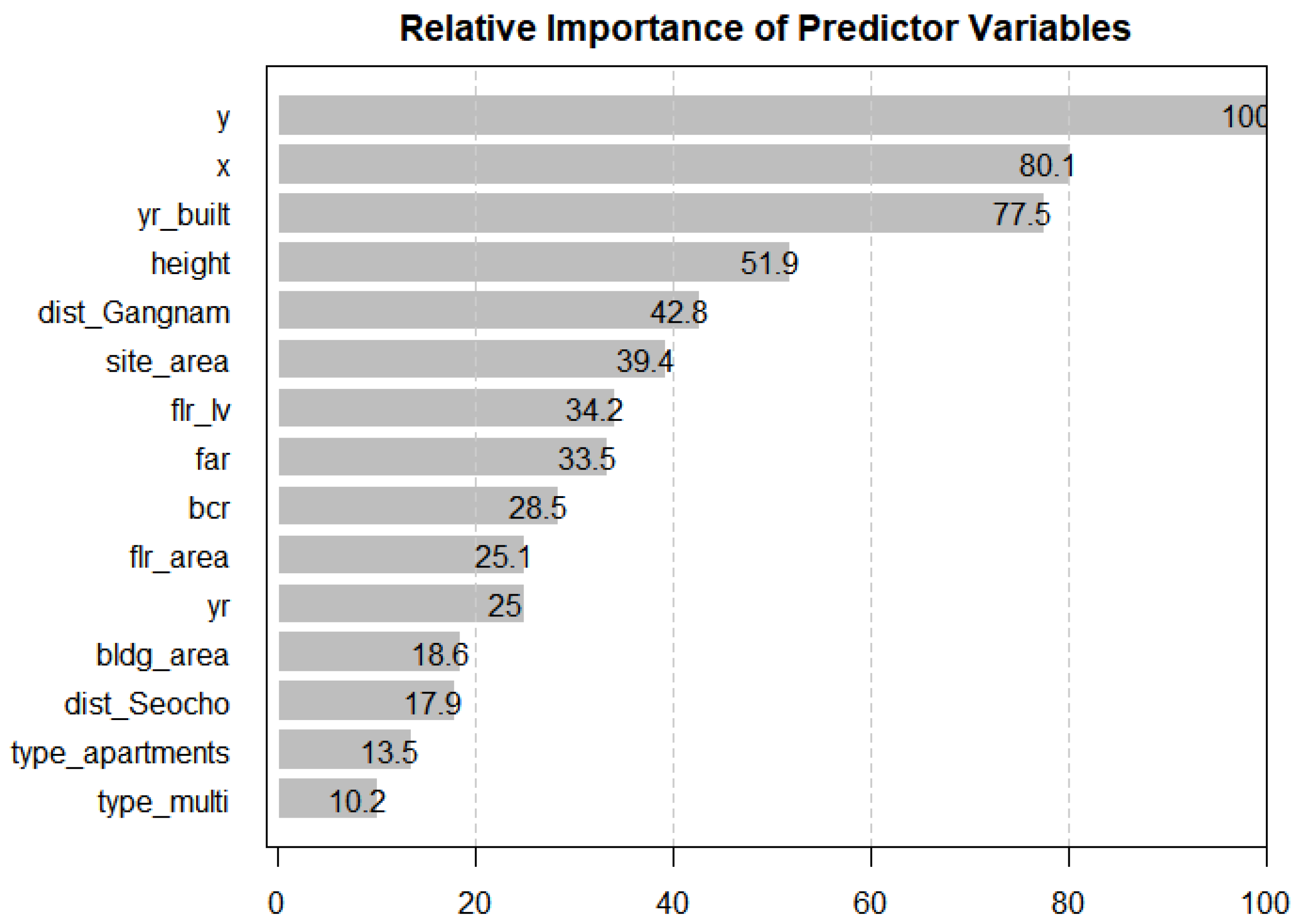
As mentioned in the previous section, the relative importance of the predictor variables in a random forest model can be calculated. This can compensate for the disadvantage of random forests, making intuitive visualization and interpretation of the results difficult.
Figure 5 shows the relative importance of the predictor variables in the selected random forest model. The most important variable, the
y coordinate, has a score of 100, and the scores of the other variables are estimated. Following the
y coordinates, the
x coordinates, the years built, the heights, and a binary variable indicating whether the building is in Gangnam-gu, one of the 25 districts in Seoul, were relatively significant. Considering that five of the listed variables (i.e., site_area, far, bcr, flr_area, and bldg_area) are area-related, the areas are one of the most important factors that affect house prices, which is consistent with the results from previous studies. In addition, the location-related variables also have considerable influences on the target variable: not only the absolute locations represented by the
x and
y coordinates but also the districts in which the properties are located seem to have a significant influence.
6. Conclusions
Although it is crucial to secure data integrity across the entire study region when utilizing spatial data, missing values almost always exist for various reasons. Several studies have been conducted to develop imputation methods for spatial data to address this problem. In geography, IDW and kriging have been commonly used, and they have contributed to solving the discontinuity of data. Recently, it has been suggested that the development of machine learning can replace existing spatial interpolation methods, and its outperformance has been demonstrated. However, there are still uncertainties about whether it can be applied to spatial data representing complex urban phenomena.
While there is a considerable number of studies that compare machine learning and the existing interpolation methods, the existing works tend to focus on the environmental fields. To fill this gap in the literature, we compared machine learning (i.e., neural networks and random forests) and spatial interpolation methods (i.e., IDW and kriging) using real estate transactions data in Seoul, South Korea. In this process, we constructed a dataset by combining the real estate transactions data and the integrated building information data. We proceeded with model optimization by varying the parameters to obtain the best results from each method.
From the maps of the residuals from each model, we found that the machine learning models performed better than the spatial imputation methods. The neural network model and the random forest model did not show high residuals across the study area. This visual impression was confirmed by a set of accuracy metrics, i.e., MAE, RMSE, MAPE, and MASE. The random forest model was the most accurate, followed by the neural network. The spatial interpolation methods showed clusters of high residuals, and kriging followed IDW in terms of the accuracy indicators. High residuals tend to appear in the regions with high transaction prices. To confirm how the selected variables affect the prediction results, the relative variable importance was calculated, and those related to areas and locations were found to have a significant influence.
In this study, we conducted a comparative analysis of machine learning and spatial interpolation methods for predicting house prices. The application of machine learning to the imputation of spatial data has been successful in many studies. Nonetheless, this study is significant as it provides more empirical evidence to support the use of machine learning for social science research and urban analytics. It is also expected that this study can contribute to the application of machine learning in the imputation of spatial data.
Nevertheless, it is important to note that this result should not be generalized to other fields of study and other types of spatial data. With the development of machine learning, many methods have been proposed, and their performance is continuously improving. However, the performance of a specific model for a specific application is affected by various factors, such as the size and structure of the data. Therefore, it is important to ensure that the method we adopt and the mode we are building are superior to other candidates through careful evaluation.


