Abstract
In order to discuss the participation selection strategy of relevant subjects in WEEE recycling, a Stackelberg game model of “recyclers—remanufacturers—government” in a WEEE recycling network is constructed, and the system’s stability strategy and conditions are analyzed. Besides this, the direct and indirect effects of recovery time sensitivity, CRMs’ life expectancy sensitivity, and government subsidies on the optimal decision-making of both recyclers and remanufacturers are explored. The results show that the system can achieve a stable and ideal equilibrium, and achieve win–win for all parties, through reasonable profit transfer and cost-sharing. The dual sensitivity of manufacturers’ demand and policy subsidies has the same qualitative impact on the decision variables of the recyclers and remanufacturers. The subsidies vary depending on the CRMs’ recovery effort level of remanufacturers, and these can incentivize the remanufacturers to increase CRMs’ life expectancy. Moreover, a cost-sharing contract between recyclers and remanufacturers can avoid “free-riding” behavior in WEEE recycling. The research can assist in the benefit coordination and behavior adjustment of WEEE recycling members, and provide a theoretical basis for governments to formulate appropriate recycling subsidies to promote the formal recycling of E-waste.
1. Introduction
In recent decades, with the rapid development of science and technology, the life cycle of electronic products has gradually shortened, generating more waste products [1,2,3,4]. It is estimated that in 2020, the global E-waste (Waste Electrical and Electronic Equipment, WEEE) generation reached a record 56.4 mt, and has become the fastest growing waste, with generation expected to reach 74.7 mt by 2030 [5,6,7]. However, only 17.4% of this waste was reasonably recycled, which means a large number of critical row materials such as copper, iron and rare metals were lost in vain. If not handled properly, these waste products will not only harm the ecological environment, but will also lead to the huge waste of resources. Moreover, informal WEEE recycling channels involving the unreasonable disposal of WEEE, such as obtaining metal materials through incineration and burying WEEE without harmless treatment, will generate more pollution, and cause the loss of resources, especially critical raw materials (CRMs), such as copper and rare metals [8,9,10,11]. More countries have not only paid attention to the quantity of WEEE recycling, but have also become concerned with the improvement of WEEE recycling quality [12,13,14,15,16]. In practice, WEEE recycling treatment has achieved remarkable resource and environmental results, driven by the fund system, but it still faces problems such as a large gap in subsidy funds, the low participation enthusiasm of remanufacturers, and the difficulty encountered by recyclers in making profits from formal recycling channel. As basic stakeholders of the WEEE recycling network, the participation strategies of remanufacturers and recyclers have a significant impact on WEEE recycling. Therefore, in view of the difficulties faced by each subject, it is important to study the interaction mechanism, stability strategy and evolution-influencing factors of the above stakeholders to regulate WEEE recycling.
The interaction of various uncertain factors exists in WEEE recycling, so remanufacturers should take the recycled products into account when formulating the production plan. For example, in the process of recycling, the life expectanies of CRMs and recycling products will directly change the production plan. On the one hand, as consumers’ pursuit of products becomes more personalized, the market life of products is shortened, resulting in the early abandonment of WEEE. Given the various uncertain factors in WEEE recycling process, it is difficult for recyclers to estimate the recycling amounts of WEEE and process them in a timely manner or in a short time, which reduces the life expectancy of CRMs. On the other hand, there is uncertainty regarding the recycling time in consumers in the recycling process. The inconsistencies in recycling time will lead to uncertainty about the remanufacturers’ processing of the raw materials required for reproduction. Therefore, the different strategic choices of stakeholders caused by the uncertainty of recycling time should be considered in the process of WEEE recycling and remanufacturing.
However, the life expectancy of CRMs has not been considered, as there is no relevant recycling standardization and subsidy policy regulation, resulting in a low CRMs recycling rate and a lower recovery time of the CRMs. How to encourage recyclers to increase the life expectancy of CRMs and how recyclers and remanufacturers can achieve Pareto optimality when there is a “bidirectional free-riding” phenomenon will be further explored. Considering the bounded rationality and the policy guidance, a Stackelberg game model between the remanufacturers and recyclers based on recovery time sensitivity and CRMs’ life expectancy sensitivity is constructed. Second, the Stackelberg model between remanufacturers and recyclers with a cost-sharing contract is constructed to analyze the dual sensitivity of manufacturers’ demand and the policy subsidy effect on the equilibrium. What are the stable strategies and realization conditions of WEEE recycling channels, how the sensitivity parameter affects the decision-making of WEEE recycling participants, and how the government guides all parties to choose participation strategies through policy formulation will become the focus of this paper. The research of this paper enriches the relevant management theories, such as the WEEE recovery cost contract theory, the WEEE recovery competition game strategy, and government regulation measures.
The remainder of this paper is organized as follows. Section 2 summarizes the literature on WEEE recycling. Section 3 provides model notations and introduces the models’ assumptions. Section 4 constructs the initial model and calculates the equilibrium solution. The influence of the measured variables on the parameters is also discussed. Section 5 discusses the optimal decisions of the two subjects under cost-sharing, which is used to solve the problem of bidirectional free-riding. Section 6 conducts simulations, and the best decision-making suggestions and most feasible cost-sharing contracts for the two bodies are discussed. Also the model’s robustness and contributions are discussed in this section. Section 7 summarizes the findings and offers suggestions for future research.
2. Literature Review
2.1. The WEEE Recycling Channel
The choice of the WEEE recycling channel (single manufacturer-led, recycler-led, third party-led, or a combination) is important. The effective selection and evaluation of recycling channels can help decision-makers choose the best way to recycle to meet demand [17,18,19,20]. Research on the WEEE recycling channel has achieved fruitful results and has provided a useful game theory reference for researching the above-mentioned problems. For example, Toyasaky et al. [21] constructed the decision models of WEEE monopolistic recycling and competitive recycling. Li et al. [22] constructed a recycling channel optimization model by mixed-integer programming and analyzed how recovery rate and recovery conditions impact the recycling channel. Savaskan et al. [23] constructed a recycling model composed of one original manufacturer and two retailers, and in addition, analyzed the recycling rate of WEEE under centralized and decentralized decision-making circumstances. In addition, research on the recycling incentive and punishment mechanism, competition between formal and informal recycling, and the cooperation mechanism of the formal WEEE recycling channel has also provided decision support for the WEEE recycling channel [24,25,26].
2.2. Government Actions on WEEE Recycling Channels
Using static and dynamic game theory analyses of the government and remanufacturers, some scholars have found that government incentive measures greatly impact the construction of WEEE recycling channels [27,28,29]. Government subsidies have an important effect on the investment threshold of the remanufacturer and recycler [30,31,32,33]. When the remanufacturer achieves economies of scale, their environmental protection awareness and ability will be increased because the remanufacturer can improve and achieve efficient and green WEEE recycling technology with government subsidies. This would generate higher environmental protection benefits. Therefore, policy incentives can encourage the remanufacturer to achieve an effective recovery of WEEE recovery systems. In addition, some scholars [34,35] have utilized game theory among the remanufacturer, governments, as well as the recycler, and the results show that only the clear sharing of responsibility among all parties, together with subsidies to remanufacturers and recyclers, can positively impact WEEE recovery. Thus, establishing a cost-sharing mechanism among the government, remanufacturer, and recycler will help effectively develop WEEE recycling.
However, most academic research on development and application has focused on enterprise management, fairness and efficiency, innovation and development, and policymaking, in which policymaking is mainly between government and enterprises, with the government regulating enterprise behaviour. However, few studies have been conducted on the application of game theory to demand time sensitivity and the life sensitivity of recycled CRMs to design WEEE recycling channels. Thus, this study fills an important gap in the literature.
In order to be closer to the reality and more deeply explore the interaction mechanisms between various stakeholders in WEEE recycling, some scholars have applied Stackelberg game theory based on irrational assumptions to the field of WEEE recycling. Therefore, considering the time sensitivity and CRMs’ life expectancy sensitivity of consumers’ demand, and the impact of subsidy policy, a Stackelberg game model between recycler and remanufacturer has been constructed. Here, the following questions are raised: What are the stable strategies and realization conditions of the WEEE recycling channel? What conditions can be met to achieve the ideal equilibrium of the WEEE recycling channel?
3. The Stackelberg Game Model of Two Stakeholders
3.1. Model Description
In this paper, a Stackelberg game is used to model the decision processes of remanufacturer and recycler, wherein the recycler is the leader and the remanufacturer is the follower, and the role of government subsidies in the remanufacturer and recycler’s decision-making is also considered. The WEEE recycling scenario is set as follows: recyclers collect WEEE and sell them to remanufacturers with WEEE processing qualifications. The remanufacturers process WEEE and recycling CRMs, and then sell CRMs to the WEEE product market. Besides this, the government subsidizes remanufacturers based on the remanufacturer’s CRMs’ recovery effort level. In order to improve the quality and timeliness of the recycled products and processed materials, remanufacturers will pay attention to the CRMs’ life expectancy and recycling time. Moreover, although there are informal E-waste recycling channels, formal recycling channels usually cooperate with informal channels to improve market competitiveness and viability.
Two Stackelberg game models are constructed in this paper; the first model is the basic model wherein there is no cost-sharing between recyclers and remanufacturers, and the second model is the cost-sharing contract model wherein recyclers and remanufacturers share a proportion of investment cost. Figure 1 illustrates the decision-making sequence for both models. As the leader in the Stackelberg game, the recyclers determine the WEEE sale price and recycling time. Remanufacturers determine the CRMs’ price and CRMs’ recovery effort level, and then the remanufacturers sell the CRMs to the WEEE product market.
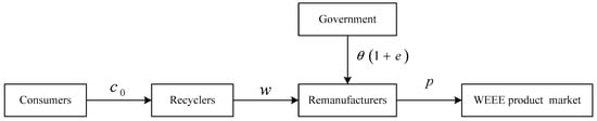
Figure 1.
Subjects of the game model.
3.2. Model Notations
The parameter variables are defined as follows:
- : potential market demand;
- : price sensitivity;
- : delivery time sensitivity;
- : CRMs’ life expectancy sensitivity;
- : remanufacturer’s recycling technology investment cost factor;
- : recycling cost per unit;
- : processing cost per unit;
- : funding policy subsidy rate;
- : fixed cost of the logistics recycling system;
- : marginal cost of compressing the recycling time;
- : proportion of recycler sharing the remanufacturer’s cost for increasing CRMs’ recovery effort level to increase the life expectancy of CRMs;
- : proportion of remanufacturer sharing the recycler’s cost for compressing recycling time;
- : remanufacturer’s pricing decision variable on the CRMs based on the WEEE sale price;
- : subsidy per unit given by the remanufacturer to recycler.
The decision variables are defined as follows:
- : WEEE sale price;
- : CRMs’ price;
- : CRMs’ recovery effort level;
- : recycling time.
3.3. Model Assumptions
#1: There are two main subjects—the recycler and remanufacturer. The recycler is responsible for recycling and transporting WEEE to the remanufacturer without WEEE treatment, and the remanufacturer is responsible for WEEE processing and CRMs restoration, and then for selling them to the WEEE product market. The recycler and remanufacturer are all bounded rationally.
#2: The potential market demand and the remanufacturer’s recycling technology investment cost factor are sufficiently large.
#3: The initial life expectancy of CRMs is 1%, and the life expectancy of CRMs is increased by increasing the investment in the CRMs’ recovery effort level. The CRMs’ recovery effort level of the remanufacturer determines the CRMs’ life expectancy.
#4: To incentivize formal recycling, the subsidy policy positively impacts the formal WEEE recycling channel, and the subsidy is variable, with an initial value of . Therefore, the unit WEEE processing subsidy is ; that is, the unit WEEE processing subsidy will change with the CRMs’ recovery effort level .
3.4. Model Construction
Due to the rapid updating of production technology and the fact that CRMs are always in short supply, remanufacturers need to purchase CRMs as soon as possible to maintain the continuity of their production links. This means that the recovery time of CRMs will affect the profits of CRMs consumers. Therefore, the recovery time of WEEE will affect the demand for CRMs. On the other hand, remanufacturers have requirements regarding the quality of CRMs. Low-quality CRMs cannot meet the remanufacturers’ production standards. They can improve the quality of CRMs by improving the recycling efforts of recyclers. Remanufacturers can evaluate the recycling quality and demand quantity of CRMs by referring to the recycling efforts of recyclers. Therefore, the CRMs’ recovery effort level will affect the CRMs demand of remanufacturers. Thus, recycling time and CRMs’ recovery effort level will influence CRMs’ demand, which are represented as and in the demand function, where is recycling time sensitivity, is recycling time, is CRMs’ life expectancy sensitivity and is CRMs’ recovery effort level. Remanufacturers are also sensitive to the price of CRMs, and the impact of CRMs’ price on demand is , where is price sensitivity. Therefore, the consumer demand in the base model is , where is the potential market demand.
Due to consumers’ requirements for recycling time, recyclers can shorten the recycling time by investing in a recycling system. The recycler’s investment cost is assumed to be , which is common in all recent papers [36,37,38,39], where is the fixed cost of the recycler’s WEEE recycling system, and is the marginal cost of compressing the recycling time of the recycler. The marginal cost of compressing one unit of recycling time increases as the recycling time decreases, and . Therefore, the total profit of the recycler is consisting with the WEEE sales profit and the investment cost of the recycling system.
where the first term is the total WEEE sales profit derived from the recycler selling WEEE to the remanufacturer, which consists of the WEEE sales revenue minus the cost of acquiring WEEE; and the second term is the recycling investment cost.
For remanufacturers, the remanufacturers purchase WEEE from the recycler at the WEEE sale price ; the remanufacturer processes the WEEE and obtain CRMs from WEEE with processing cost per unit , and sell CRMs at CRMs’ price ; remanufacturers can obtain profit from WEEE processing, which is equal to . Simultaneously, the government will give remanufacturers a unit subsidy that refers to the remanufacturer’s CRMs’ recovery effort level, and the unit subsidy is , where is the initial funding policy subsidy. Therefore, remanufacturers will invest in improving the CRMs’ recovery effort level, and the expenditure is , where is the remanufacturer’s recycling technology investment cost factor. In all, the profit gained by the remanufacturer is consistent with the profit derived from selling CRMs and the investment in the CRMs’ recovery effort. The remanufacturer’s profit is:
4. Results
4.1. Equilibrium Points
The Stackelberg model is solved by reverse induction, and the optimal decision, demand, and profit of the two subjects are listed in Table 1 (Appendix A).

Table 1.
Equilibrium in the Stackelberg game model.
4.2. The Impact of Changes on the Optimal Decision
Proposition 1:
. If , . If , . If ,.
Where and are as follows:
When manufacturers are not time-sensitive (), the recycler will have more time to collect WEEE products without worrying about the impact on manufacturers. The recycler can have a better time effect with less cost. The indirect impact of delivery time sensitivity is that the optimal CRMs’ recovery effort level will decrease. Simultaneously, the remanufacturer will derive an indirect benefit from the recycler, whereby they can invest more to shorten the recycling time. When the demand for CRMs from the manufacturers increases due to the recycler shortening the recycling time, the number of CRMs sold by the remanufacturer increases. In other words, there is a “free-riding” behavior, whereby the remanufacturer free-rides on the recycler’s investment. Therefore, the remanufacturer will save costs by reducing technology investment. As investment decreases, the CRMs’ recovery effort level decreases (Appendix B).
When the manufacturers’ delivery time sensitivity reaches a certain level (), the effect of shortening the recycling time gradually decreases, and the marginal cost of shortening the recycling time increases. The recycler will reduce the recycling time further by reducing profits. To maintain the demand of manufacturers, the remanufacturer will increase technological investment to increase CRMs’ recovery effort level, and thus increase the life expectancy of CRMs. The remanufacturer is willing to increase investment in the WEEE recovery technology, but this will generate more customer demand. When the manufacturers’ delivery time sensitivity reaches , the cooperation between recycler and remanufacturer reaches the optimal level. Considering the marginal profit obtained from increasing demand, which is generated from the increased investment in compressing the recycling time and increasing the CRMs’ recovery effort level to increase the life expectancy of CRMs, the marginal cost of each entity’s investment is acceptable. When the sensitivity is large enough (), the investment cost required for each additional unit of demand is much higher than the benefit. Therefore, the remanufacturer will reduce the technology input, and the CRMs’ recovery effort level will be reduced.
4.3. The Impact of Changes on the Optimal Decision
Proposition 2:
,.
When manufacturers show higher sensitivity to the life expectancy of CRMs, the remanufacturer will invest more money to increase life expectancy, and then the government can provide more financial subsidies to the remanufacturer. However, funding subsidies will not continue to grow because excessive funding subsidies will increase the government’s financial pressure; in other words, the government will consider the marginal benefit derived from the subsidy spent when the marginal benefit is equal to 0 or it is negative, and the subsidy will no longer increase. If manufacturers become more sensitive to the life expectancy of CRMs, that is, the value of the parameter increases, the demand for WEEE recycling products will increase. That is, the remanufacturer is willing to improve their CRMs’ recovery technology. If the government wants to promote WEEE recycling to reduce environmental pollution and promote sustainable development, it will increase financial subsidies. Our research can offer policy adjustment suggestions useful for promoting sustainable development and resource reuse, as well as reference conditions for establishing closed-loop WEEE recycling channels and resource sharing among entities (Appendix C).
As the subsidy increases, the recycling time will be shortened, so the subsidy indirectly affects the optimal recycling time. First, to expand the sales market and obtain more subsidies, the remanufacturer will increase processing technology expenditures. As the remanufacturer increases their investment in recovery technology, the CRMs’ recovery effort level also increases, as does the demand for the recycler. To meet market demand, the remanufacturer will require the recycler to shorten the recycling time. Second, when the expenditure reaches equilibrium, the marginal cost of further improving the recovery technology will be higher. The remanufacturer will require the recycler to increase investment in logistics recovery systems to maintain demand. In this case, the recycling time will be shortened.
4.4. The Impact of Changes on the Optimal Decision
Proposition 3:
.
Proposition 3 shows that the manufacturers’ sensitivity to the life expectancy of CRMs directly affects the recycling time. The CRMs’ life expectancy sensitivity is higher, and the recycling time is shorter. Because the remanufacturer will increase CRMs’ recovery effort level to increase the life expectancy of CRMs to meet the requirements of manufacturers, part of the CRMs’ life expectancy growth costs will be passed on to manufacturers and the recycler in the form of higher CRMs unit prices or lower WEEE recycling prices. To make up for the loss of demand caused by the increase in the unit price of CRMs and the loss of profit caused by the decrease in the sales price of WEEE, the recycler will compress the recycling time to shorten the delivery time, thereby increasing the sales of WEEE ( Appendix D).
4.5. Cost-Sharing Contract Model under Changes
From the above analysis, we obtain a cross effect between the parameters of two game subjects. Owing to the dual sensitivity of demand, both parties are motivated to engage in bidirectional free-riding. Specifically, when the recycler shortens the recycling time to decrease delivery time by increasing investment, the demand from manufacturers will increase, and the remanufacturer can profit by increasing demand without increasing investment. Similarly, when the remanufacturer increases the investment in the CRM’s recovery effort level to increase the life expectancy of CRMs, the demand will increase, and the recycler can also profit without more investment. To explore the stable relationship between the two subjects and optimal cooperative decision-making, we constructed a cost-sharing contract model, which will be explained in the next section.
Owing to the dual sensitivity of demand, increasing investment in technology by either the recycler or the remanufacturer will simultaneously increase their profits. In fact, this is bidirectional free-riding, and either subject is willing to free-ride to increase their own market demand and save costs. To solve this problem, and to explore how to build a solid relationship between recycler and remanufacturer and further build WEEE recycling channels, a cost-sharing contract model is constructed.
In this cost-sharing contract model, it is assumed that is the proportion of recyclers sharing the remanufacturer’s cost for increasing the CRM’s recovery effort level to increase the life expectancy of CRMs, and is the proportion of remanufacturers sharing the recycler’s cost for compressing the recycling time to shorten the delivery time. Moreover, it is assumed that the proportion of recyclers sharing the remanufacturer’s cost for increasing the life expectancy of CRMs is not 1, because when the parameter is 1, recyclers will choose to recycle and process WEEE without cooperating with the remanufacturer, and then sell the CRMs to manufacturers, which will increase their profits. In contrast, when the proportion of remanufacturers sharing the recycler’s cost for compressing recycling time is 1, i.e., the remanufacturer shares all the investment, the recycling time is shortened, and there is no investment required for the recycler. Thus, the remanufacturer will choose to recycle WEEE separately, without the process by which the recycler recycles WEEE and sells it to the remanufacturer. When either or equal 0, the cost-sharing model is transformed into a one-way cost-sharing model. When all the cost-sharing is 0, the recycler and remanufacturer each bear its own cost; this situation has been analyzed in Section 4.
After adding a bidirectional cost-sharing contract to the initial profit function, the recycler’s profit model is:
The profit model of the remanufacturer after joining the bidirectional cost-sharing contract is:
Using the reverse induction method to solve the Stackelberg game model, the optimal decision, demand, and profit of both subjects are obtained. Table 2 displays the results (Appendix E).
Table 2.
Optimal results of two subjects under the cost-sharing contract model.
5. Model Simulations
To determine the relationship between variables and verify the models, a simulation comparing the decisions of WEEE recycling stakeholders under the game model without a cost-sharing contract and under a cost-sharing contract is analyzed. The following basic parameters are set, with reference to [13] and [3] and taking into account the actual CRMs’ recovery effort level, recycling time, and profit of the recycler and remanufacturer.
The values of the parameters/variables are: unit/month, /unit, , /day, /unit, /unit, , unit/day, unit, and .
5.1. Game Model without a Cost-Sharing Contract
The research results in Figure 2 and Figure 3 show that CRMs’ life expectancy sensitivity and policy subsidies significantly impact CRMs’ recovery effort level, and the impact is positive. From Figure 2, we can see that as manufacturers increase their sensitivity to CRMs’ life expectancy, CRMs’ recovery effort level increases. The indirect effect is that an increase in the delivery time sensitivity of manufacturers reduces the life expectancy of CRMs. Figure 3 illustrates that when the remanufacturer receives more funding subsidies, the life expectancy of CRMs is longer. In addition, when the CRMs’ life expectancy sensitivity is higher, the CRMs’ recovery effort level is simultaneously higher.
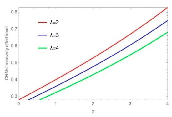
Figure 2.
Impact of on .
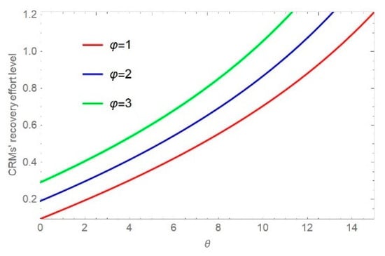
Figure 3.
Impact of on .
Figure 4 and Figure 5 illustrate the impact of delivery time sensitivity on the CRMs’ recovery effort level and recycling time under different values of the parameter by increasing time sensitivity. Figure 4 also shows the indirect effect of the CRMs’ life expectancy sensitivity on the recycling time. As manufacturers become delivery time-sensitive, i.e., the parameter increases, the recycling time decreases. The CRMs’ life expectancy sensitivity indirectly affects the recycling time: when manufacturers are time-insensitive, i.e., the parameter is close to 0, the indirect effect of on delivery time is similar. As manufacturers exhibit more delivery time sensitivity, the indirect effect of CRMs’ life expectancy sensitivity on delivery time is different, and the effects of different values of CRMs’ life expectancy sensitivity on the recycling time are obvious. With the same value of time sensitivity, the recycling time becomes shorter as the value of the CRMs’ life expectancy sensitivity becomes larger. In addition, Figure 5 shows that the CRMs’ recovery effort level first decreases then increases.
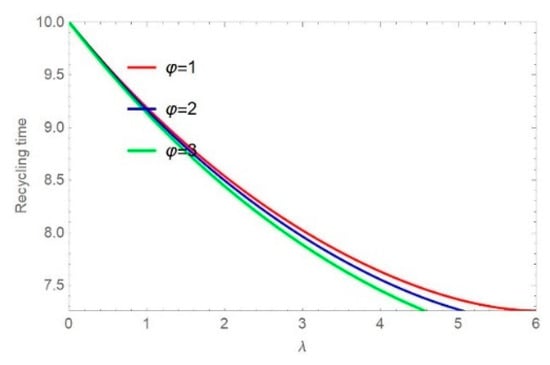
Figure 4.
Impact of on .
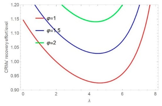
Figure 5.
Impact of on .
The results in Figure 6 and Figure 7 show that government funding subsidies increase, recycling time decreases, and the delivery time decreases as recycling time is shortened. As the CRMs’ life expectancy sensitivity and delivery time sensitivity increase, the recycling time becomes shorter for the same subsidy. Figure 8 and Figure 9 show that as the CRMs’ life expectancy sensitivity increases, the recycling time decreases. As the parameter increases, the recycling time decreases, i.e., the delivery time also decreases. Similarly, as the subsidy and delivery time sensitivity increase, the recycling time becomes shorter for the same value of the CRMs’ life expectancy sensitivity.
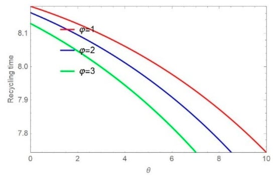
Figure 6.
Impact of on .
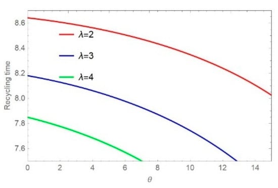
Figure 7.
Impact of on .
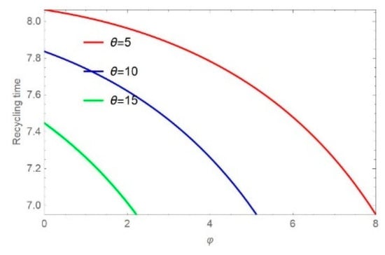
Figure 8.
Impact of on .
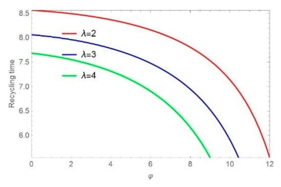
Figure 9.
Impact of on .
5.2. Cost-Sharing Contract Model
Here, we use the same parameter settings as the initial model to simulate the cost-sharing contract model and compare the changes in sharing coefficients to the change trends of benefits of all subjects with and without cost-sharing. To ascertain the trend, we selected different intervals of the parameters and in each figure. The graphics of the three-dimensional decision variables were plotted using Mathematical 12.0 software.
Figure 10 shows that with the increase in cost-sharing, the CRMs’ recovery effort level gradually increases. Via the equilibrium solutions obtained by backward induction (Table 2), we obtained the following result: when the remanufacturer shares more of the cost with the recycler, i.e., parameter increases, the CRMs’ recovery effort level increases, but the increasing trend of parameter is not obvious. Moreover, more cost-sharing of the CRMs’ recovery effort level will increase the life expectancy of CRMs.
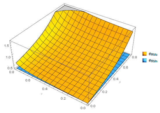
Figure 10.
Comparison of under different models.
Figure 11 shows the recycling time with and without a cost-sharing contract. Recycling time affects delivery time, and they are positively correlated, so delivery time will be reduced by changing the cost-sharing coefficient to shorten the recycling time. By observing the relationship between the cost-sharing coefficient and recycling time, we can offer the following reasoning: when the proportion of the remanufacturers sharing the recycler’s cost for compressing the recycling time is low, the proportion of recyclers sharing the remanufacturer’s cost for increasing the CRMs’ recovery effort level to increase the life expectancy of CRMs is higher, the increase in the proportion of recyclers sharing the remanufacturer’s cost and the decrease in the proportion of the remanufacturers sharing the recycler’s cost will reduce recycling time. When the proportion of remanufacturers sharing the recycler’s cost for compressing recycling time is higher, the proportion of recyclers sharing the remanufacturer’s cost for increasing the life expectancy of CRMs is lower, and the optimal decision of the two subjects is to bear their own costs.
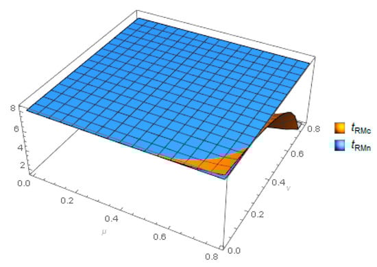
Figure 11.
Comparison of under different models.
Figure 12 shows that as the proportion of remanufacturers sharing the recycler’s cost increases, the CRMs demand simultaneously increases. The recyclers share the remanufacturer’s cost of improving the CRMs’ life expectancy. The demand first increases, then decreases. The higher the cost-sharing rate, the greater the cross-impact of parameters and . Thus, the optimal decision for the two subjects is to cooperate.
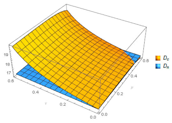
Figure 12.
Comparison of under different models.
Figure 13 depicts how the parameters and impact the trend of recycler’s benefits. The second-order partial derivative of the recycler’s profit relative to the parameter is negative; that is, . This means that when , the recycler’s profit function is concave. This is because when recyclers share the remanufacturer’s investment in improving CRMs’ life expectancy to increase the degree of the remanufacturer’s CRMs’ recovery effort level, the recycler can have more funds to improve WEEE recycling technology, thereby increasing the recycling value and efficiency of CRMs. With further increases in the parameter , the benefits generated by the cost-sharing of the life expectancy of CRMs decrease, reducing the profits of recyclers. Given bidirectional cost-sharing, when is in the range (0–1), the recycler’s profit under cost-sharing is higher than the separate costs, so it is profitable for the recycler to share the remanufacturer’s cost, and the profit increases with the increase in parameter . The increase in parameter means that the recycler will share more WEEE transportation costs. Through the profit analysis of the recycler, we have concluded that the best decision of the recycler is to cooperate with the remanufacturer.
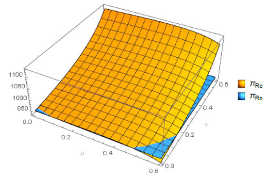
Figure 13.
Comparison of under different models.
From the profit comparison of the remanufacturer (Figure 14), we see that when the cost-sharing coefficient is close to zero, the profit of the remanufacturers under cost-sharing is greater than the costs of both subjects. This means that if the cost sharing rate is high, unless the remanufacturer gives up certain benefits to establish a stable supply–demand relationship, the remanufacturer usually will not cooperate with the recycler. If the cost-sharing factor is close to 1, the profit of the remanufacturer will decrease sharply, and the remanufacturer will choose to establish their own WEEE recycling channel.
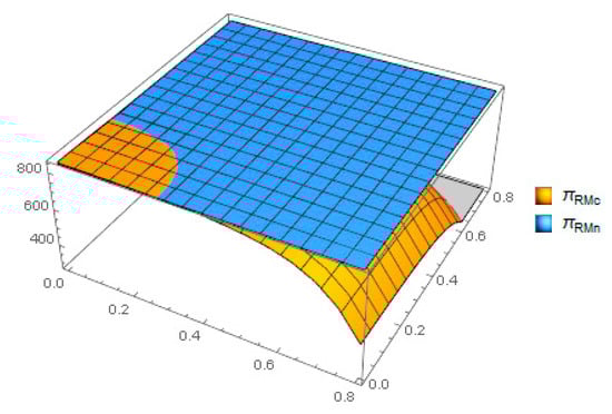
Figure 14.
Comparison of under different models.
In summary, the simulation model and parameter assignment of our study are appropriate. We analyzed the current situation of WEEE recycling and CRMs recovery and provide suggestions about policy subsidies and achieving cooperation between the recycler and remanufacturer. By further combining the profit analysis of the recycler and remanufacturer, we have found that the optimal decision value of the parameters and is between . This result also explains the status of WEEE recycling in related regions where recycling and reusing WEEE occur, and reveals the urgency of improving the situation, such as in China. The informal recycler collects WEEE and sells it to the formal remanufacturer, and the formal remanufacturer undertakes a certain percentage of the recycling costs of the recycler. The ratio is determined by the recycler and the remanufacturer through negotiation. The remanufacturer will not share too much of the transportation costs because they have many partners, or they can establish WEEE recycling systems separately.
Figure 15 shows that comparing different values of , the profit with cost-sharing is higher than the profit without. In addition, the threshold of parameters and can also be observed (a). When parameters and do not exceed the threshold, the benefits of cost-sharing outweigh the benefits without cost-sharing (b–d).
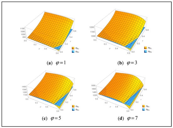
Figure 15.
Comparison of under different values of ( ).
By observing Figure 16, the same conclusions can be drawn. If the remanufacturer does not share the recycler’s cost for compressing recycling time () or the recycler does not share remanufacturer’s cost for increasing the CRMs’ recovery effort level to increase the CRMs’ life expectancy(a). When the WEEE product market is more sensitive to the CRMs’ life expectancy, delivery time, and WEEE subsidy, the threshold of parameters and varies (b–d). However, there is still a suitable range of cost-sharing coefficients to enable one subject to achieve Pareto improvement, whereby both subjects are better off. The verification results indicate that cost-sharing can effectively help two subjects achieve Pareto optimality. As shown in Figure 15 and Figure 16, if the remanufacturer does not share the recycler’s cost for compressing recycling time (), when the WEEE product market shows more sensitivities to CRMs’ life expectancy, there the cost-sharing coefficient fluctuates to make the benefits of the two subjects under cost-sharing greater than those without cost-sharing. Similarly, if the recycler does not share the remanufacturer’s cost for increasing the CRMs’ recovery effort level (), when the CRMs’ life expectancy sensitivity increases, the two subjects more easily achieve Pareto optimality because the threshold of the cost-sharing coefficient increases.
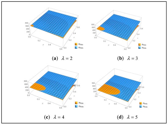
Figure 16.
Comparison of under different values of ( ).
6. Discussion
6.1. Model Extensions
To explore an actual situation of WEEE recycling and the robustness of our cost-sharing model, we took China’s WEEE recycling market as the research object, given its higher percentage of informal recycling, and in China the formal processor and informal recycler have established cooperation such that the remanufacturer as the formal processor gives a subsidy to the recycler to save transport cost, and the informal recycler transports WEEE to the remanufacturer, increasing profit. Based on the results of our research, the recycler and remanufacturer can establish cooperation via a cost-sharing contract, with which an informal recycler can utilize the WEEE recycling channel to increase the quantity of WEEE recycling and transport WEEE to the remanufacturer, who manufactures the CRMs products. This can reduce the time required for WEEE recycling and increase the demand from manufacturers, who are time-sensitive, which in turn will increase the profit of the recycler and remanufacturer, thereby increasing the possibility of constructing a formal WEEE recycling system. At the same time, the formal remanufacturer provides subsidies to informal recycling sectors to stabilize their cooperative relations. The remanufacturer chooses partners and determines the recycling price of WEEE products and CRMs according to their own needs. The remanufacturer will give subsidies to a recycler who chooses to cooperate.
To increase the model’s accuracy, we assumed that the subsidy that the remanufacturer grants to the recycler varies with manufacturer’s demand, rather than remaining fixed. In addition, the WEEE sales prices offered to the recycler will be affected by market fluctuations in CRMs, so the investment in WEEE recycling channels, such as transportation by the recycler, remains unchanged. The remanufacturer will decide the price of CRMs by considering the previous manufacturer’s demand before the remanufacturer process and the sale of CRMs, based on the WEEE sale price (which is decided by the recycler), the remanufacturer’s price for the added value of their processing of WEEE, and the remanufacturer’s expected benefit of selling CRMs to manufacturers. We assumed that the remanufacturer’s price for the added value of their processing of WEEE, plus their expected benefit, is ; the CRMs price provided by the remanufacturer to the manufacturers is , and the unit subsidy given by the remanufacturer to the recycler is .
The demand function and the profit function of both subjects are:
The Stackelberg game model was solved by the reverse induction method, and the optimal solutions of the extended model were obtained. Table 3 displays the results (Appendix F).
Table 3.
Results of two subjects under model extensions.
Proposition 4:
, , , , .
If , then ; if , then ; if , then .
Proposition 4 verifies that under the new power structure, when the remanufacturer is the leader, the interaction between the recycler and the remanufacturer is qualitatively the same as the interaction in the initial model. The delivery time sensitivity and the CRMs’ life expectancy sensitivity of manufacturers and policy subsidies have the same qualitative impact on the decision variables of the recycler and remanufacturer. This indicates that the model established in this study is robust.
6.2. Contributions
Because the CRMs are in short supply and essential for remanufacturers’ production, remanufacturers need to receive CRMs early to keep their products from becoming obsolete, which means recycling time will influence the recyclers and remanufacturers’ profit, while WEEE recycling time is ignored. Moreover, subsidies given to the WEEE collector are already considered [15,16,36], and the results of the research are that the subsidy can incentivize WEEE collectors to be willing to take a formal approach via formal ways. However, the value of the subsidy is always fixed, and the specific utility of the subsidy in WEEE recycling cannot be obtained. Thus, the recycling time expectancy and the CRMs’ life expectancy are considered and added in the game model in this paper, and a variable subsidy and cost-sharing contract model between remanuffacturers and recyclers are propose to avoid free-riding. According to the setting of parameters [15,16,36], the trajectory trend of the CRMs’ life expectancy and the recovery time expectation under variable subsidies and fixed subsidies are drawn out in Figure 17 and Figure 18.
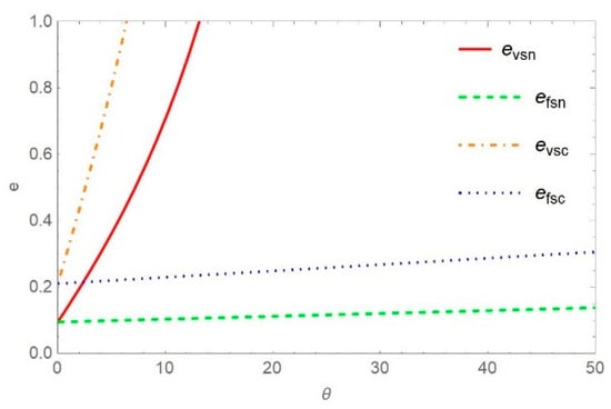
Figure 17.
The influence of on with a fixed subsidy and a variable subsidy .
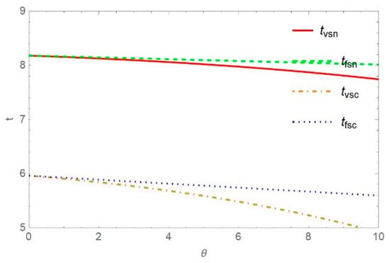
Figure 18.
The influence of on under fixed subsidy and variable subsidy .
Figure 17 shows the trajectory trend of the CRMs’ life expectancy sensitivity under a variable subsidy and a fixed subsidy, where means the CRMs’ recovery effort level under variable subsidy and there is no cost-sharing construct between recyclers and remanufacturers, means the CRMs’ recovery effort level under fixed subsidy and no cost-sharing construct, means the CRMs’ recovery effort level under variable subsidy and cost-sharing construct, and means the CRMs’ recovery effort level under fixed subsidy and cost-sharing construct. It can be seen that the CRMs’ life expectancy gradually increases with time evolution in both modes, and finally tends to be stable. However, the CRMs’ life expectancy under variable subsidy mode is higher than that under fixed subsidy mode. This shows that supply chain members’ investment in WEEE recycling will increase the CRMs’ life expectancy, so the construction of a WEEE recycling network is a positive behavior. In a WEEE recycling network where the government provides a variable subsidy model, remanufacturers have higher CRMs’ life expectancies than fixed subsidy models. This is because the government adopts a variable subsidy to share the recycling cost of the remanufacturer, thereby increasing the recycling enthusiasm of the remanufacturer, and at the same time, it will encourage the remanufacturer to increase its recycling input, which will directly and positively affect the CRMs’ life expectancy. Thus, the cooperation of government and remanufacturers to actively participate in WEEE recycling can maximize the CRMs’ life expectancy. However, under the fixed subsidy model, the core of the remanufacturer’s operation is the product market, which does not affect the CRMs’ life expectancy. Therefore, when the government provides a fixed subsidy, the profit brought in by the remanufacturer’s fixed subsidy does not improve the CRMs’ life expectancy. The above shows that the cooperation between remanufacturers and government can improve their own profits and the CRMs’ life expectancy, and establish a good corporate image. Moreover, the cooperation between recyclers and the government can increase the supply to the WEEE recycling market and indirectly increase the CRMs’ life expectancy.
As Figure 18 shown, variable subsidies can effectively shorten the recycling time, and the cost-sharing contract can decrease the recycler’s optimal recycling time, where means recycling time under variable subsidy and there is no cost-sharing construct between recyclers and remanufacturers, means recycling time under fixed subsidy and no cost-sharing construct, means recycling time under variable subsidy and cost-sharing construct, and means recycling time under fixed subsidy and cost-sharing construct. Under variable subsidy and cost-sharing conditions, the recycler and remanufacturer can obtain more profit because the demands of manufacturers are positively correlated with the CRMs’ life expectancy and negatively correlated with the recovery time. It can be seen that both fixed subsidy utility and variable subsidy utility decrease with the increase in recycling time, and eventually tend to be stable. This suggests that the existence of recycling time expectations has a negative impact on the WEEE recycling network, which can compromise the utility of governments and remanufacturers. It can also be seen from the above figure that the total utility of the government and remanufacturers under the cost-sharing model is higher than that of the government and remanufacturers under the fixed cost model, which fully demonstrates the feasibility of variable government subsidies and cost-sharing.
7. Conclusions
This paper constructs a Stackelberg game model of the WEEE recycling network, including recyclers, remanufacturers and the government, discusses the selection of WEEE recycling participation strategies of various stakeholders, and analyzes the decision-making problems under conditions of recycling time sensitivity, the CRM’s life expectation sensitivity, and government regulation. Finally, some meaningful conclusions are drawn from numerical simulations.
The decision-making of recyclers and remanufacturers is a long-term dynamic game process. The Stackelberg stability of the decision-making of both groups is affected by various uncertain factors, and it will gradually develop after repeated games. The government punishment and subsidy mechanisms can effectively encourage recyclers and remanufacturers to carry out remanufacturing activities, as well as reducing the impact of recovery time sensitivity and CRM’s life sensitivity on WEEE recycling, and the incentive effect of the punishment mechanism is more significant than that of the subsidy mechanism. First, when the recovery time sensitivity increases, it will further increase the difficulty of remanufacture if the government sets too a high treatment fund. At this time, the government should increase the intensity of financial incentives, stabilize the impact of recovery time sensitivity on WEEE recycling by adjusting subsidies to recyclers, and encourage remanufacturers and recyclers to actively participate in WEEE recycling. When the recovery time sensitivity is reduced, the uncertainty of the recovery market is reduced, and recyclers can stabilize WEEE the recovery strategy by improving the recovery effort level. Second, when the CRM’s life expectancy sensitivity is high, it is difficult for remanufacturers to benefit from WEEE recycling. In this circumstance, the government should adopt positive environmental regulation policies and increase incentives to regulate remanufacture activities. With the gradual development of WEEE recycling, the government should adjust policies and improve the acceptance of remanufactured products. At this time, appropriate government regulations and punishments will further reduce the CRMs life expectancy sensitivity. In addition, compared with the impact of government regulation, the cost-sharing contract is more conducive to improving the overall benefits of WEEE recycling. The coordination of stakeholders is conducive to reducing free-riding and promoting the implementation of government policies, further improving the level of product remanufacturing and WEEE recycling profits. Thus, the cost-sharing contract model constructed in this paper is robust.
The government can promote the CRMs’ recovery effort level of the remanufacturer and reduce WEEE recycling using the variable subsidy we have designed, which means WEEE can be recycled and processed by qualified ways, and the government can save money spent on resource recovery and reduce the environmental pollution generated by remanufacturer’s WEEE processing. The reducing of recycling time means the idle WEEE can be quickly and effectively processed.
Based on the research contents and the main conclusions above, some suggestions to help governments enhance their managerial insights have been put forward. First, an internal R&D cooperation mechanism among stakeholders should be constructed in the WEEE recycling network. Second, the government should actively supervise the behavior of recyclers and improve the enthusiasm of remanufacturers to provide remanufactured products by reducing time sensitivity. Third, the government should set a reasonable subsidy level to improve the CRM’s life expectancy, which can effectively encourage recyclers to improve their recycling efforts, promote the development of remanufacturing and enhance social welfare. Last, in the product design stage, the recyclable performance of products should be fully considered to maximize the CRM’s life expectancy, which is not only conducive to the recycling of WEEE, but also reduces the cost and technical inputs in the remanufacturing process. This conclusion has important theoretical and practical significance for the improvement of WEEE remanufacturing benefits.
However, this study discusses subsidies primarily for WEEE stakeholders, such as recyclers or remanufacturers. How the subsidies impact other stakeholders (such as consumers) of the WEEE recycling network should be addressed in future research. In addition, the dynamic design of a government variable subsidy mechanism also needs further discussion.
Author Contributions
Conceptualization: Q.S.; data collection, integration, and analysis: S.-H.L.; writing—original draft: S.-H.L.; writing—review and editing: Q.S. and S.-H.L.; funding acquisition: Q.S. All authors have read and agreed to the published version of the manuscript.
Funding
Project ZR2020MG069 supported by Shandong Provincial Natural Science Foundation.
Institutional Review Board Statement
Not applicable.
Informed Consent Statement
Not applicable.
Data Availability Statement
Not applicable.
Acknowledgments
We would like to thank the anonymous reviewers and the handling editor of this paper who contributed to improving the quality of this paper. We thank LetPub (www.letpub.com) for linguistic assistance and the pre-submission expert review.
Conflicts of Interest
The authors declare no conflict of interest.
Appendix A
Proof of Table 1:
To find the partial derivative of Equation (3), we have
Then the Hessian matrix of the re-manufacturer is
Obviously, the profit function of the re-manufacturer is concave because , in which the remanufacturer’s recycling technology investment cost factor is relatively large compared to the other parameters. Let and .
Then we obtained
We brought the parameters and into Equation (2), and gained the profit function of the recycler, which is .
Similarly, it can be found that
The Hessian matrix of the recycler is
The profit function of the recycler is negative if . As we suppose that the value of the remanufacturer’s recycling technology investment cost factor is bigger than other parameters, we focused on the order of parameter k, and we determined that the inequality is true. Further, let and ; we have the optimal solution of the recycler’s profit function, as follows:
Then we substitute and into the parametric formula
and we obtain the optimal decisions of the remanufacturer:
Finally, by substituting , , and into Equations (1)–(3), we derive the benefits under the optimal decisions of the recycler and the remanufacturer, as follows:
and
□
Appendix B
Proof of Proposition 1:
From Table 2, we see that
Similarly, the remanufacturer’s recycling technology investment cost factor and the potential market demand are relatively large compared to the other parameters, therefore
Further,
and
Obviously, .
If , ; if , ; if , . is a convex quadratic function, and we can get its zero point by . We have
which are positive under the condition of
Finally, we have the monotonic relationship between the crucial raw materials’ life rate, which increases the effort level and the manufacturers’ sensitivity to the recycling time, as follows:
If , then ; if , then ; if , then , where
□
Appendix C
Proof of Proposition 2:
From Table 2, we see that the crucial raw materials’ life rate increases the effort level:
The first-order partial derivative of with respect to and is
The remanufacturer’s recycling technology investment cost factor and the potential market demand are relatively large compared to the other parameters, and the first part is positive and the absolute value of that is greater than the absolute value of the second part. Therefore, .
From Table 2, we see that
Similarly, we can construct
and then the simplified function is
and the monotonic relationship between and is:
If , then ; if , then ; if , then .
It is easy to find that is a convex quadratic function, and we obtain the solution of :
which are both possible when
Because the remanufacturer’s recycling technology investment cost factor and the potential market demand that we assumed are large enough, the above equation and its required conditions can be fulfilled. We combine our previous assumptions ( and are large enough, and ) and the results obtained to infer that if , then . □
Appendix D
Proof of Proposition 3:
From Table 2, we have determined that
Obviously, since the potential market demand is relatively large and the values of other parameters are positive, then . Further, .
From Table 2, we see that the crucial raw materials’ life rate increases the effort level
and the first-order partial derivative of with respect to and is
The remanufacturer’s recycling technology investment cost factor and the potential market demand are relatively large compared to the other parameters, and the first part is positive and the absolute value of that is greater than the absolute value of the second part. Therefore, .
From Table 2, we have
Because and are large enough compared to the other parameters, . □
Appendix E
Proof of Table 2:
The certification process in Table 3 is similar to that in Table 2. Since the leader of the Stackelberg game is the recycler, we use the reverse order induction method to solve the model. First, according to Equation (5), we can obtain
from which we obtain the Hessian matrix of the remanufacturer:
Therefore, one can conclude that the profit function of the remanufacturer is concave if . Let and , we have
Then, substituting and into Equation (4), we obtain the reclaimer’s profit function:
Similarly, it is easy to find
Then we can have the Hessian matrix of the recycler:
one can conclude that the profit function of the recycler is concave because is much greater than zero. Letting and , we have
Then we substitute and into the parametric formula
and , and we can derive the optimal decisions of the re-manufacturer:
Further, by substituting , , and into Equations (4) and (5), we gain
□
Appendix F
Proof of Table 3:
To test the robustness of the model, we take the remanufacturer as the leader of the Stackelberg game. When the remanufacturer is the leader, the recycler determines the collection time and the wholesale price first. We assume the manufacturer price for CRMs provided by the recycler, based on the market conditions of WEEE and its output. The subsidy per unit given by the remanufacturer to the recycler is . In this situation, we add the price of the remanufacturer selling the CRM to the manufacturers , and the subsidy per unit to the model.
From Equation (7), we have
Then, we have the Hessian matrix of recycler: . Hence, one can conclude that the profit function of the recycler is concave if . Letting and , we have
Take
We have the Hessian matrix of the remanufacturer, which is:
Letting and , we have:
By substituting and into the recycler’s response functions, we gain the recycler’s optimal decisions, as follow:
Then, we take , , and into Equations (6)–(8), and we have the profits of the remanufacturer and recycler under optimal conditions: ,
□
Proof of Proposition 4:
From Table 3, we have
As we assumed before, parameters and are sufficiently large; therefore,
Further,
Similarly,
then .
Similarly, the remanufacturer’s recycling technology investment cost factor and the potential market demand are relatively large compared to the other parameters, which lead to and
since the potential market demand and the remanufacturer’s recycling technology investment cost factor are sufficiently large and other parameters are positive,
We use two methods to derive the monotonic relationship between the crucial raw materials’ life rate increased effort level and the recycling time sensitivity , by which we can verify that the previous method of solving the monotonic relationship by simplifying the function is feasible.
1. Let directly. We have
2. We denote
, which is a convex function, then .
If , then ; if , then ; if , then . Letting , we have
From the derivation above, we have and , which are possible since
Then, we have the monotonic relationship between the crucial raw materials’ life rate increased effort level and the recycling time sensitivity, as follows:
If , then ; if , then ; if , then . □
References
- Ameli, M.; Mansour, S.; Ahmadi-Javid, A. A simulation-optimization model for sustainable product design and efficient end-of-life management based on individual producer responsibility. Resour. Conserv. Recycl. 2019, 140, 246–258. [Google Scholar] [CrossRef]
- Ardi, R.; Leisten, R. Assessing the role of informal sector in WEEE management systems: A System Dynamics approach. Waste Manag. 2016, 57, 3–16. [Google Scholar] [CrossRef]
- Bai, Q.; Xu, J.; Chauhan, S.S. Effects of sustainability investment and risk aversion on a two-stage supply chain coordination under a carbon tax policy. Comput. Ind. Eng. 2020, 142, 106324. [Google Scholar] [CrossRef]
- Chang, X.; Wu, J.; Li, T.; Fan, T.-J. The joint tax-subsidy mechanism incorporating extended producer responsibility in a manufacturing-recycling system. J. Clean. Prod. 2019, 210, 821–836. [Google Scholar] [CrossRef]
- Charles, R.G.; Douglas, P.; Dowling, M.; Liversage, G.; Davies, M.L. Towards Increased Recovery of Critical Raw Materials from WEEE– evaluation of CRMs at a component level and pre-processing methods for interface optimisation with recovery processes. Resour. Conserv. Recycl. 2020, 161, 104923. [Google Scholar] [CrossRef]
- Fang, Y.; Wei, W.; Liu, F.; Mei, S.; Chen, L.; Li, J. Improving solar power usage with electric vehicles: Analyzing a public-private partnership cooperation scheme based on evolutionary game theory. J. Clean. Prod. 2019, 233, 1284–1297. [Google Scholar] [CrossRef]
- Fu, J.; Zhong, J.; Chen, D.; Liu, Q. Urban environmental governance, government intervention, and optimal strategies: A perspective on electronic waste management in China. Resour. Conserv. Recycl. 2020, 154, 104547. [Google Scholar] [CrossRef]
- Gu, Y.; Wu, Y.; Xu, M.; Wang, H.; Zuo, T. To realize better extended producer responsibility: Redesign of WEEE fund mode in China. J. Clean. Prod. 2017, 164, 347–356. [Google Scholar] [CrossRef]
- Gu, Y.; Wu, Y.; Xu, M.; Wang, H.; Zuo, T. The stability and profitability of the informal WEEE collector in developing countries: A case study of China. Resour. Conserv. Recycl. 2016, 107, 18–26. [Google Scholar] [CrossRef]
- Hou, J.; Zhang, Q.; Hu, S.; Chen, D. Evaluation of a new extended producer responsibility mode for WEEE based on a supply chain scheme. Sci. Total Environ. 2020, 726, 138531. [Google Scholar] [CrossRef]
- Islam, M.T.; Huda, N. Reverse logistics and closed-loop supply chain of waste electrical and electronic equipment (WEEE) /E-waste: A comprehensive literature review. Resour. Conserv. Recycl. 2018, 137, 48–75. [Google Scholar] [CrossRef]
- Kastanaki, E.; Giannis, A. Dynamic estimation of future obsolete laptop flows and embedded critical raw materials: The case study of Greece. Waste. Manag. 2021, 132, 74–85. [Google Scholar] [CrossRef] [PubMed]
- Li, X.; Mu, D.; Du, J.; Cao, J.; Zhao, F. Game-based system dynamics simulation of deposit-refund scheme for electric vehicle battery recycling in China. Resour. Conserv. Recycl. 2020, 157, 104788. [Google Scholar] [CrossRef]
- Li, Y.; Wei, C.; Cai, X. Optimal pricing and order policies with B2B product returns for fashion products. Int. J. Prod. Econ. 2012, 135, 637–646. [Google Scholar] [CrossRef]
- Liu, T.; Cao, J.; Wu, Y.; Weng, Z.; Senthil, R.A.; Yu, L. Exploring influencing factors of WEEE social recycling behavior: A Chinese perspective. J. Clean. Prod. 2021, 312, 127829. [Google Scholar] [CrossRef]
- Liu, Y.; Quan, B.-T.; Xu, Q.; Forrest, J.Y.-L. Corporate social responsibility and decision analysis in a supply chain through government subsidy. J. Clean. Prod. 2019, 208, 436–447. [Google Scholar] [CrossRef]
- Lu, B.; Yang, J.; Ijomah, W.; Wu, W.; Zlamparet, G. Perspectives on reuse of WEEE in China: Lessons from the EU. Resour. Conserv. Recycl. 2018, 135, 83–92. [Google Scholar] [CrossRef]
- Morris, A.; Metternicht, G. Assessing effectiveness of WEEE management policy in Australia. J. Environ. Manag. 2016, 181, 218–230. [Google Scholar] [CrossRef]
- Munerah, S.; Koay, K.Y.; Thambiah, S. Factors influencing non-green consumers’ purchase intention: A partial least squares structural equation modelling (PLS-SEM) approach. J. Clean. Prod. 2021, 280, 124192. [Google Scholar] [CrossRef]
- Pekarkova, Z.; Williams, I.D.; Emery, L.; Bone, R. Economic and climate impacts from the incorrect disposal of WEEE. Resour. Conserv. Recycl. 2021, 168, 105470. [Google Scholar] [CrossRef]
- Saha, S.; Sarmah, S.; Moon, I. Dual channel closed-loop supply chain coordination with a reward-driven remanufacturing policy. Int. J. Prod. Res. 2016, 54, 1503–1517. [Google Scholar] [CrossRef]
- Savaskan, R.C.; Wassenhove, L.V. Reverse channel design: The case of competing retailers. Manag. Sci. 2016, 52, iv-154. [Google Scholar] [CrossRef] [Green Version]
- Savaskan, R.C.; Bhattacharya, S.; Van Wassenhove, L.N. Closed-Loop Supply Chain Models with Product Remanufacturing. Manag. Sci. 2004, 50, 239–252. [Google Scholar] [CrossRef] [Green Version]
- Shan, H.; Yang, J. Promoting the implementation of extended producer responsibility systems in China: A behavioral game perspective. J. Clean. Prod. 2019, 250, 119446. [Google Scholar] [CrossRef]
- Sharpe, L.M.; Harwell, M.C.; Jackson, C.A. Integrated stakeholder prioritization criteria for environmental management. J. Environ. Manag. 2021, 282, 111719. [Google Scholar] [CrossRef]
- Shittu, O.S.; Williams, I.D.; Shaw, P.J. Global E-waste management: Can WEEE make a difference? A review of e-waste trends, legislation, contemporary issues and future challenges. Waste Manag. 2021, 120, 549–563. [Google Scholar] [CrossRef]
- Sun, Q.; Wang, C.; Zuo, L.; Lu, F.-H. Digital empowerment in a WEEE collection business ecosystem: A comparative study of two typical cases in China. J. Clean. Prod. 2018, 184, 414–422. [Google Scholar] [CrossRef] [Green Version]
- Tong, X.; Wang, T.; Chen, Y.; Wang, Y. Towards an inclusive circular economy: Quantifying the spatial flows of e-waste through the informal sector in China. Resour. Conserv. Recycl. 2018, 135, 163–171. [Google Scholar] [CrossRef]
- Toyasaki, F.; Boyacι, T.; Verter, V. An Analysis of Monopolistic and Competitive Take-Back Schemes for WEEE Recycling. Prod. Oper. Manag. 2011, 20, 805–823. [Google Scholar] [CrossRef]
- Wang, J.; Wang, Y.; Liu, J.; Zhang, S.; Zhang, M. Effects of fund policy incorporating Extended Producer Responsibility for WEEE dismantling industry in China. Resour. Conserv. Recycl. 2018, 130, 44–50. [Google Scholar] [CrossRef]
- Wang, Y.; Wang, Z.; Li, B.; Liu, Z.; Zhu, X.; Wang, Q. Closed-loop supply chain models with product recovery and donation. J. Clean. Prod. 2019, 227, 861–876. [Google Scholar] [CrossRef]
- Wang, H.; Gu, Y.; Li, L.; Liu, T.; Wu, Y.; Zuo, T. Operating models and development trends in the extended producer responsibility system for waste electrical and electronic equipment. Resour. Conserv. Recycl. 2017, 127, 159–167. [Google Scholar] [CrossRef]
- Wang, Z.; Wang, Q.; Chen, B.; Wang, Y. Evolutionary game analysis on behavioral strategies of multiple stakeholders in E-waste recycling industry. Resour. Conserv. Recycl. 2020, 155, 104618. [Google Scholar] [CrossRef]
- Wu, Y.; Li, H.; Gou, Q.; Gu, J. Supply chain models with corporate social responsibility. Int. J. Prod. Res. 2017, 55, 6732–6759. [Google Scholar] [CrossRef]
- Zhang, D.; Cao, Y.; Wang, Y.; Ding, G. Operational effectiveness of funding for waste electrical and electronic equipment disposal in China: An analysis based on game theory. Resour. Conserv. Recycl. 2020, 152, 104514. [Google Scholar] [CrossRef]
- Zhang, J.; Chiang, W.-Y.K.; Liang, L. Strategic pricing with reference effects in a competitive supply chain. Omega 2014, 44, 126–135. [Google Scholar] [CrossRef]
- Zhang, X.-Q.; Yuan, X.-G.; Zhang, D. Research on Closed-Loop Supply Chain with Competing Retailers under Government Reward-Penalty Mechanism and Asymmetric Information. Discret. Dyn. Nat. Soc. 2020, 2020, 1–20. [Google Scholar] [CrossRef] [Green Version]
- Zhang, X.-M.; Li, Q.-W.; Liu, Z.; Chang, C.-T. Optimal pricing and remanufacturing mode in a closed-loop supply chain of WEEE under government fund policy. Comput. Ind. Eng. 2021, 151, 106951. [Google Scholar] [CrossRef]
- Zuo, L.; Wang, C.; Sun, Q. Sustaining WEEE collection business in China: The case of online to offline (O2O) development strategies. Waste Manag. 2020, 101, 222–230. [Google Scholar] [CrossRef]
Publisher’s Note: MDPI stays neutral with regard to jurisdictional claims in published maps and institutional affiliations. |
© 2022 by the authors. Licensee MDPI, Basel, Switzerland. This article is an open access article distributed under the terms and conditions of the Creative Commons Attribution (CC BY) license (https://creativecommons.org/licenses/by/4.0/).