Geospatial Analysis of Land Use/Cover Change and Land Surface Temperature for Landscape Risk Pattern Change Evaluation of Baghdad City, Iraq, Using CA–Markov and ANN Models

Abstract

Understanding future landscape risk pattern change (FLRPC) scenarios will help people manage and utilize natural resources. In this study, we have selected a variety of landscape and anthropogenic factors as risk parameters for FLRPC assessment. Land use/cover change (LUCC) and land surface temperature (LST) are regarded as significant factors that have resulted in large-scale environmental changes. Result analysis of the previous LUCC from 1985 to 2020 showed that construction land and water body (WB) increased by 669.09 and 183.16 km², respectively. The study continues to predict future LUCC from 2030 to 2050, in which the result has shown that a large land use conversion occurred during the future prediction period. In addition, the LST forecasting analysis illustrated that the previous LST maximum and minimum are 38 °C and 15 °C, which will be increased to 40.83 °C and 26.25 °C in the future, respectively. Finally, the study used the weighted overlay method for the FLRPC analysis, which applies analytic hierarchy process techniques for risk evaluation. The FLRPC result demonstrated that Baghdad City is in the low-risk and medium-risk to high-risk categories from 2020 to 2050, while AL and BL are in the very-high-risk categories. Meanwhile, WB and NG have always been safe, falling into the very-low-risk and low-risk categories from 2020 to 2050. Therefore, this study has successfully assessed the Baghdad metropolitan area and made recommendations for future urban development for a more safe, resilient, and sustainable development.

1. Introduction

Human socio-economic activities, the connection between human population growth and general urban developmental tendency, have caused significant variations in the enlargement of all cities worldwide and jeopardized the land use/cover change (LUCC) sustainability of the city area and land surface temperature (LST) change in regional and global contexts [1,2]. According to the United Nations (UN) prediction, urban areas will outnumber rural areas in terms of population by 60% by 2050 [3]. One of the main causes of the rapid LUCC is the increasing urban population, which has increased the demand for settlement and agricultural land in almost every country throughout the world [4,5]. Many natural land covers have been destroyed and converted into other land use types, such as agricultural land, urban land, and other human uses. The land transformation from one land use character to another is known as LUCC, and it occurs as a result of the composited connection between anthropogenic factors and the environment [6]. LUCC is regarded as a major contributor to global environmental change, having a significant effect on LST change, ecosystem change, biodiversity cycle, and biodiversity [7]. These variations have a direct influence on landscape ecological deprivation and biodiversity loss, soil resource degradation, the effect on the land surface, greenhouse gas emissions, and global climate change [8,9,10]. The LUCC research is regarded as a significant aspect in determining the parameters that are responsible for regional environmental variations, landscape changes, landscape fragmentation, ecosystem changes, climate changes, urbanization, sustainable development, and environmental risk evaluation of cities [11,12]. Based on the problems that existed in the destructive urbanization landscape, and what will be changed in the future, the answerable factors to these changes must be determined by modeling future LUCC and LST, which are the two major drivers of urban landscape variation.

Multiple landscapes with anthropogenic factors were identified for risk valuation in this study to better understand the landscape risk pattern change. The historical and future changes in LUCC and LST are the key parameters for this study [13,14]. Knowing the past and future variations in LUCC and LST in future urbanization is significant [15]. This tool is invaluable for analyzing the causes and consequences of changes to support the LUCC and LST [16]. Several models, including multiagent models, hybrid models, analytical equation-based models, expert system models, statistical models, evolutionary models, cellular models, and Markov models, have been widely used in previous LULC studies, and modeling emphasized the analysis of the consequences of land use variation [17]. This study uses the Cellular Automata–Markov (CA–Markov) model, which is widely used in current research and provides a viable technique for the spatiotemporal dynamic simulation of LUCC in complex systems [13,18]. The Markov chain model is an application that forecasts future land use direction in a particular area based on the change rates in the past land use [19,20,21]. The LUCC modeling technique is a comprehensive system that can process numerous layers of data integration, such as geospatial and remote sensing data and socio-economic data [22]. The LST is difficult to simulate and forecast in a nonlinear and chaotic urban context by using time-series remote sensing images [23,24]. Soft prediction techniques, such as CA, Markov chains, and Logistic Regression, are examples of this type of method used in this research [25]. The Artificial Neural Network (ANN) has proven to be effective in situations such as these when the underlying mechanisms are not well understood; for instance, when the tendency within the phenomena is known, the Markov chain is preferable due to the insufficient geographical dependence and spatial dispersion of the phenomena [26]. The ANN model is as a component of deep learning technologies and it was initially designed to accurately simulate the underpinning working mechanism of the human brain in the learning process and interpret complicated real-world patterns [27]. The use of the ANN model becomes compelling when the underlying processes and linkages are difficult to explain and exhibit chaotic features.

Many studies have effectively and successfully employed the Markov model for future LUCC analysis for research sites and purposes. Dey et al. [28] predicted the LUCC in Raj Shahi City, Bangladesh, by using the Markov chain model. Guan et al. [29] studied the land use change and landscape ecology in Kitakyushu by using the Markov model. Kumar et al. [30] analyzed the LUCC simulation by using the Markov model and remote sensing data of the city. Faichia et al. [15] predicted the land use change scenario in Vientiane based on the CA–Markov with RS–Geographical Information System (GIS) technologies through GIS and Markov model simulation of LUCC prediction in Amman by H. A. Khawaldah. Although a number of researchers have evaluated and predicted the global LUCC, several studies concentrating on the Baghdad environment in Iraq obtained normal findings, while most of the existing research only focused on the previous LUCC. No research on future urban land use for environmental sustainability has been found.

In Iraq, most studies focused on the previous to present LUCC, with no research concentrating on future urban land conversion and environmental sustainability. Mohamedmeki et al. [31] studied the land use change toward sustainability in Baghdad City, Iraq. Qassim et al. and Al-Ramahi et al. analyzed the LUCC from 1986 to 2019. The spatial concentration of Radon Gas distribution in Baghdad City was assessed by using RS and GIS [32]. Hamdy et al. [33] mapped the LUCC in Al-Karkh, Baghdad. This study has classified and examined the LUCC and LST causes, processes, and effects, with an emphasis on urban development to guarantee livelihood and the environment in better and sustainable development in the research region. Nath et al. [34] used RS and GIS technologies to analyze the LUCC and environmental risk assessment in Dujiangyan City (Southwest China) and future potential landscape risks based on the CA–Markov model and AHP process assessment [35]. However, a study analyzing and predicting the LUCC and ecological risk in Baghdad, Iraq, has not been found. In this study, the future landscape risk pattern change (FLRPC) scenarios were studied by using remote sensing and GIS analysis tools. The landscape pattern risk assessment is mainly based on the LUCC and LST integrated with landscape factors. The FLRPC of the area was characterized by multi-source and multi-receptor effects, and the mechanisms of exposure and interference are complex. In addition, the landscape pattern risk studies for future scenarios in the selected study area are challenging.

A risk assessment that focuses on future landscape risk hazards from human activity and natural phenomena can be measured for sustainability by identifying risk areas through analysis [36]. The factors that threaten urban development sustainability and stability in the region are taken into consideration [37]. The FLRPC assessment can study the association between regional risk sources and risk receptors by using a landscape pattern framework as a reference for ecological risk control in the future and help encourage a better understanding of the set of factors exposed to the ecological environment in the region [28]. This study aims to examine and characterize the historical LUCC dynamics from 1985 to 2020 and model its FLUCC from 2030 to 2050 to effectively promote and develop the sustainability of ecosystems in the region. Moreover, this study is designed to analyze previous changes in LST and its scenario from 2030 to 2050 based on the LUCC data. Finally, the LUCC and LST with landscape factors have been collected for the FLRPC analysis. This simulated FLRPC will aid urban planners and land use decision-makers in designing solutions for suitable urbanization in Baghdad through a comprehensive understanding of the current situation and future development possibilities and environmental security.

2. Materials and Methods

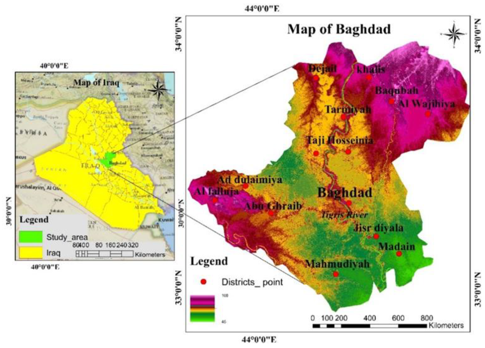
2.1. Study Area

Baghdad (the capital of Iraq) has been selected as the study area. There are 12 districts across the city limits in the northeast, namely Khalis, Baqubah, Al Wajihiya, and Dejail in the northwest [38]. Tarmiyah, Hosseinia, and Taji are in the north, Abu Ghraib and Jisr Diyala are in the southwest and east, Mahmudiyah and Madain are in the southeast, and Ad Dulaimiya and Al Falluja are in the western districts of Baghdad [38], as shown in Figure 1. Baghdad has a population density of 931.4 people per km², with a total area of 7669.69 km² and a variety of land uses. The research study site is located between latitudes 33°19′ and 33°32′ N and longitudes 44°24′ and 44.40° E. Baghdad is the second-largest city after Cairo, which is the biggest Arabic city in western Asia. The elevations and slope are ranked above the mean sea level (MSL) of 25 m to 109 m, with an average slope of 0°–89.89°, as shown in Figure 1.

Baghdad is the most populated city in Iraq, with majority of the population residing there [39]. Baghdad’s population increased at an alarming rate over the last 70 years (between 1950 and 2020), starting with 579,167 people in 1950 and consistently increasing to 3,606,844 people in 1985, with its population exponential growth reaching 7,144,260 by 2020 [40]. There are concerns that future urban development may be threatened by natural disasters; however, the US Geological Survey Earthquake datasheet from 1985 to 2020 (https://earthquake.usgs.gov/earthquakes/search/ [accessed on 8 March 2021]) showed no reported earthquakes and fault lines in the study area, while the adjacent cities and eastern Iraq were at risk of earthquakes [32].

2.2. Data Sources

The vector (shapefile) data used in this study were obtained from the Iraqi Ministry of Education and include the polygons, data, and locations in the shapefile for each suburban district [41]. The maps were produced from the country’s vector data with a scale 1:10,000,000 [42].

This research used two Landsat-5 Thematic Mapper (TM) images and one image from Landsat-8 Operation Land Imager (OLI) sensors for this investigation, with a focus on cloud coverage, seasons, and phenomena of less than 5% [43,44].

Table 1. Detail of data sources used in the study.

Satellite	Sensor	Resolution (m)	Path/Row	Acquisition Date	Season	Cloud Cover (%)	LST	Calibration Constant for LST
							Bands	K1	K2
Landsat5	TM	30 × 30	169/037	20 July 1985	Dry	0	6	607.76	1260.56
Landsat5	TM	30 × 30	169/037	29 July 2000	Dry	2	6	666.09	1282.71
Landsat8	OLI-TIRS	30 × 30	169/037	22 August 2020	Dry	1.17	10	774.88	1321.08
ASTER DEM with the 30 m spatial resolution was obtained from the satellite images.
Google Earth Pro (GEP) with a 15 m spatial resolution was used for spatial visualizing the correct location and time.
Road shapefiles in Baghdad City was derived from the OpenStreetMap (https://www.openstreetmap.org/ (accessed on 20 February 2021).
Geological map was collected from the world geologic map https://data.apps.fao.org/map/catalog (accessed on 15 March 2021).
River shapefile was used to display the landscape intersection, which was extracted from Landsat OLI using GIS 10.8.
Soil data were obtained from FAO digital soil map of the world http://www.fao.org/soils-portal/data (accessed on 15 March 2021).
Population statistic data were collected from https://worldpopulationreview.com (accessed 20 March 2021).

Note: TM_Thematic Mapper and OLI_Operation Land Imager. ASTER DEM_Advanced Spaceborne Thermal Emission and Reflection Radiometer Digital Elevation Model.

shows the specific satellite data and other technical specifications. The corrected position verification in LUCC categorization was also performed using the GEP with a 15 m resolution [44]. We were able to determine the correct location by comparing the Landsat pictures with GEP data in both windows after the GEP data were processed by the Google Earth Engine (GEE) and QGIS.

Predicted Population Growth

The population statistical data from 1985 to 2020 were collected from the website https://worldpopulationreview.com (accessed on 1 March 2021). Population density (PD) is mainly calculated by population by area and it is expressed in population per kilometer. The population projections for 2030, 2040, and 2050 are shown in

Table 2. Statistics of historical and predicted population in Baghdad, Iraq.

Years	1985	2000	2020	2030	2040	2050
Populations	3,606,844	5,199,948	7,144,260	9,365,109	12,456,369	15,986,568

, which are calculated based on Equations (1) and (2).

The annual population increase will largely influence the natural resource reduction, settlement expansion, and LUCC removal. The population projections for 2030, 2040, and 2050 are calculated using Equations (1) and (2).

$$P_t=P_0{e}^{rt}$$

(1)

where $P_t$ denotes the population in (t) time, $P_0$ is priority population in (0) time, r is the growth rate, and t denotes time.

$$\begin{gathered} r=\frac{\Delta N}{\Delta t} \\ \Delta N=P_n-;\Delta t=t_n-t_0 \end{gathered}$$

(2)

$P_n$ denotes the population in the latest year, $P_0$ is a population of priority, $t_n$ is time in n year, and $t_0$ is time in priority year.

2.3. Methodology

2.3.1. Image Processing, Historical LUCC Classification, and Kappa Coefficient Calculation

Numerous techniques and software, such as ArcGIS, ENVI, ERDAS, and QGIS, have been used for the LUCC pre-processing to ensure the correct interpretation of the temporal dynamics and geometric compatibility with other sources [45]. In this study, the image classification and interpretation used the combined classification method based on ERDAS IMAGINE 2015 and ArcGIS 10.8. The combined method, which included supervised and unsupervised classification methods, is widely used for LUCC classification [15,32]. The maximum likelihood algorithm is the most frequently employed approach for remote sensing image interpretation using supervised classification, and it calculates the subsequent probabilities of fitting pixels to their corresponding classes according to the Bayes Theorem [46]. The WGS_1984_UTM_ZONE_48N coordinate system is used in these images. Google Earth Pro (GEP) is a crucial tool for classifying these images and visualizing the correct location and time.

The previous LUCC classification of this study yielded results with over 85% accuracy in the kappa index and overall correctness. However, if the correctness of each LUCC classification is over 85%, then the result is agreed upon for future LUCC projects. The kappa coefficient (K) is calculated by using Equation (3) [45].

$$\mathrm{K}=\frac{{{\displaystyle \sum }}_{\mathrm{i}=1}^{\mathrm{r}}{\mathrm{x}}_{\mathrm{ii}}-{{\displaystyle \sum }}_{\mathrm{i}=1}^{\mathrm{r}}\left({\mathrm{x}}_{\mathrm{i}+}\times {\mathrm{x}}_{+\mathrm{i}}\right)}{{\mathrm{N}}^2-{{\displaystyle \sum }}_{\mathrm{i}=1}^{\mathrm{r}}({\mathrm{x}}_{\mathrm{i}=1}\times {\mathrm{x}}_{+\mathrm{i}})},$$

(3)

where K represents the kappa, N defines the total number of sites in the matrix, r is the number of rows in the matrix, ${\mathrm{x}}_{\mathrm{ii}}$ is the number in row i and column i, ${\mathrm{x}}_{+\mathrm{i}}$ is the total for row i, and ${\mathrm{x}}_{\mathrm{i}+}$is the total for the column.

2.3.2. LUCC Prediction Using the CA–Markov Model

Currently, the Markov model has been frequently used in LUCC prediction research [47]. The model can predict the possibility of a trend from the first image to the last image to determine the trend of change in future LUCC probabilities based on the specific year. The Markov model was processed to create a transfer matrix and the possibility of a future transfer matrix [48].

The Markov model is a set of states $\mathrm{s}=\left\{{\mathrm{s}}_0,{\mathrm{s}}_1,{\mathrm{s}}_2,\dots ,{\mathrm{s}}_{\mathrm{n}}\right\}$. In this study, the recent state is S_t, which is transferred to the S_j state in the next step, with the probability indicated by the P_ij transformation. Thus, the state S _{(t + 1)} in the system can be classified by the previous step S_t in the Markov, as demonstrated in Equations (4) and (5).

$$\begin{gathered} {\mathrm{P}}_{\mathrm{ij}}=\left[\begin{array}{ccc}{\mathrm{P}}_{11}{\mathrm{P}}_{12}& \cdots & {\mathrm{P}}_{1\mathrm{n}}\\ ⋮& ⋮& ⋮\\ {\mathrm{P}}_{\mathrm{n}1}{\mathrm{P}}_{\mathrm{n}2}& \cdots & {\mathrm{P}}_{\mathrm{nn}}\end{array}\right], \\ 0<{\mathrm{P}}_{\mathrm{ij}}<1\mathrm{and}{\displaystyle \sum }_{\mathrm{j}=1}^{\mathrm{n}}\mathrm{Pij}=1,\mathrm{i},\mathrm{j}=1,2,3\dots \mathrm{n}, \end{gathered}$$

(4)

$${\mathrm{S}}_{\mathrm{t}+1}={\mathrm{P}}_{\mathrm{ij}}\times {\mathrm{S}}_{\mathrm{t}},$$

(5)

where P denotes the likelihood matrix in Markov; ${\mathrm{P}}_{\mathrm{ij}}$is the likelihood of changing from the current state i to another state j in the next period; S stands for the land use status, t; and t+1 expresses the time point.

The CA is the bottom dynamic transformation model integrated with the spatiotemporal dimension by increasing the modeling direction [49]. The model allows for the achievement of complexity in time–space and distinct state. The CA can determine and predict the spatial variation processes in the land use change simulation [50]. The model includes cells, cell spacing, neighbors, rules, and time. The CA model is filtered to detect neighbors. The larger the distance between the middle and the neighbor, the greater the weight factor, as demonstrated in Equation (6).

$$S_{t+1}=f\left(S_t,N\right),$$

(6)

where S defines a set of restricted cell states; t and t + 1 are the first and subsequent years, respectively; N represents the neighborhood of the cell; and f is the local area change rule.

2.3.3. Driver Variable Determination and Model Validation for LUCC Prediction

Multiple influencing driver factors are considered from the natural feature and human activities, which are the independent and dependent variables [15]. The dependent variables, such as digital elevation model (DEM), slope, road network, road distance, distance from the urban, distance from the river, and population density. The other independent variables, such as BL change to CL, WB change to CL, AL change to CL, and change from all LU to CL, are accounted as driving factors for the Land Change Modeler (LCM) in this study [32] (Figure A1a–l).

In this research, the past LUCC classification from 1985 to 2020 was processed by using ArcGIS, and the CA–Markov model was applied for future LUCC predictions for 2030, 2040, and 2050 using Terrset software [32]. The LCM window is used for data managing in Terrset software [15].

The CA–Markov model was used for future LUCCs, where the kappa coefficient values were determined to be within −1 to 1. The value descriptions kappa ≤ 0.5, 0.5 ≤ kappa ≤ 0.75, and 0.75 ≤ kappa < 1 indicate a low exception, a medium exception, and a very high exception [51,52]. These values are represented by Equations (7)–(9).

$$\mathrm{Kappa}\mathrm{for}\mathrm{no}\mathrm{information}{\mathrm{K}}_{\mathrm{no}}=\frac{\left({\mathrm{M}}_{\left(\mathrm{m}\right)}{\mathrm{N}}_{\left(\mathrm{n}\right)}\right)}{\left({\mathrm{P}}_{\left(\mathrm{p}\right)}-{\mathrm{N}}_{\left(\mathrm{n}\right)}\right)},$$

(7)

$$\mathrm{Kappa}\mathrm{for}\mathrm{location}{\mathrm{K}}_{\mathrm{location}}=\frac{\left({\mathrm{M}}_{\left(\mathrm{m}\right)}{\mathrm{N}}_{\left(\mathrm{n}\right)}\right)}{\left({\mathrm{P}}_{\mathrm{m}}-{\mathrm{N}}_{\left(\mathrm{n}\right)}\right)},$$

(8)

$$\mathrm{Kappa}\mathrm{standard}{\mathrm{K}}_{\mathrm{standard}}=\frac{\left({\mathrm{M}}_{\left(\mathrm{m}\right)}{\mathrm{M}}_{\left(\mathrm{n}\right)}\right)}{\left({\mathrm{P}}_{\left(\mathrm{p}\right)}-{\mathrm{N}}_{\left(\mathrm{n}\right)}\right)},$$

(9)

where N_(n) is no data, M_(m) is medium grid cell level data, and P_(p) is the complete grid cell data.

2.4. LST Forecasting Method

2.4.1. LST Extraction from Landsat Images

The thermal data from Landsat (TM and OLI) Images are stored as digital numbers (DNs). The guidelines conducted by the USGS were utilized to convert DNs into brightness temperature for achieving LST [53]. Then, all the three images from 1985, 2000, and 2020 were further processed in the LST retrieval tool in ArcGIS 10.8. The cell statistics tool was used to integrate the results. Equations (10)–(19) are used for LST extraction. In the first stage, extraction of LST from the (TM and OLI) images was carried out following the Landsat 8 user manual. The DNs are transformed into spectral radiance using Equation (10):

𝐿𝜆= 𝐺 𝑟𝑒𝑠𝑐𝑎𝑙 𝑒 ∗ (𝑄𝐶𝐴𝐿 + 𝐵𝑟𝑒𝑠𝑐𝑎𝑙𝑒)

(10)

This formula can also be expressed in Equation (11) as follows:

$$L\mathit{\lambda }=\left(\frac{\mathrm{LM}\mathrm{AX}\mathsf{\lambda }-\mathrm{LM}\mathrm{I}\mathrm{N}\mathsf{\lambda }}{\mathrm{QC}\mathrm{ALMAX}-\mathrm{QC}\mathrm{ALMIN}}\right)* \left(\mathrm{QCAL}-\mathrm{QCALM}\mathrm{I}\mathrm{N}\right)+\mathrm{LM}\mathrm{I}\mathrm{N}\mathit{\lambda },$$

(11)

where Lλ represents the spectral radiance, QCAL represents the volume and pixel value of the data set (DN), QCALMIN represents the minimum pixel value of the quantized and calibrated data set, and QCALMAX sets the maximum pixel value of the volume and calibration of the data set (DN) [54].

We were able to transform the DN into spectral radiance in this research using Equation (11). Equation (12) was used to convert spectral radiance to satellite brightness temperature, with the calibration constants acting as the conversion factor [55]. The temperature was converted to degrees Celsius by subtracting 273.15 from the reading.

$$\mathrm{BT}=\left(\frac{\mathrm{K}2}{\ln \left(\frac{\mathrm{K}1}{\mathrm{L}\mathsf{\lambda }+1}\right)}\right)-273.15$$

(12)

BT is the effective satellite light temperature in degrees Celsius, K₁ defines the calibration constant 1, K₂ denotes the calibration constant 2, and L denotes the spectral radiance of the satellite. Table 1 lists the thermal calibration constants for the various temperature ranges.

Several researchers were involved in the remainder of the LST retrieval procedure. The NDVI determinants are vital in the evaluation of the LST for Landsat OLI images because the result depends on the NDVI, shown in Equation (13) [56].

$$\mathrm{NDVI}=\left(\frac{\mathrm{Band}5-\mathrm{Band}4}{\mathrm{Band}5+\mathrm{Band}4}\right)$$

(13)

Equation (14) is the last step of retrieving emissivity-corrected LST.

$$\mathrm{LST}=\frac{\mathrm{BT}}{\left[1+\left(\mathsf{\lambda }\times \mathrm{BT}\mathsf{\rho }\right)\times \ln \left(\mathrm{LSE}\right)\right]}$$

(14)

where λ stands for the respective wavelength of the bands.

2.4.2. Characteristics of the LST

Several indicators are produced to provide a more accurate assessment of the changes in LST in the research region. In terms of monitoring vegetation conditions, the normalized difference vegetation index (NDVI) was developed by Rouse and colleagues (1974) [57], and it can be calculated by using Equation (15). The standard deviation built-up index is a frequently used indicator for built-up area extraction that was improved by the use of the normalized difference built-up index (NDBI) (Equation (16)). We have introduced the normalized difference water index (NDWI) to distinguish open water features from satellite images (Equation (17)). The normalized difference bareness index (NDBaI) was developed to identify bare land from other land uses (Equation (18)). Table 1 contains detailed information on the bands that were utilized. The cell statistics tool is used to integrate the indices generated from three Landsat images taken throughout each year.

$$\mathrm{NDVI}=\frac{\mathrm{NIR}-\mathrm{Red}}{\mathrm{NIR}+\mathrm{Red}}$$

(15)

$$\mathrm{NDBI}=\frac{\mathrm{SWIR}-\mathrm{NIR}}{\mathrm{IR}+\mathrm{NIR}}$$

(16)

$$\mathrm{NDWI}=\frac{\mathrm{Green}-\mathrm{NIR}}{\mathrm{Green}+\mathrm{NIR}}$$

(17)

$$\mathrm{NDBaI}=\frac{\mathrm{SWIR}-\mathrm{TIRS}}{\mathrm{SWIR}+\mathrm{TIRS}}$$

(18)

2.4.3. Conceptualization and Network Modeling of the ANN

The ANN model is used on the basis of the principle of Feed Forward Back Propagation [58]. In the hidden and output layers, every neuron adds up the weighted input vectors, and a bias constant is fed to it. Then, the result is transferred via the transfer function to create the output. This concept is illustrated in Figure 2.

2.4.4. Performance and Model for ANN Prediction

The LST-predicted processing was requested for the supported variables, such as DEM, slope, and hill shape (Figure A1). Then, the estimated output was compared with the observed LST data set. Subsequently, estimates were made for future epochs by using the network retention parameters trained in 2030, 2040, and 2050 and provided in the Section 3. The forecasting of LST in the QGIS was carried out through the MOLUSCE plugin contained in the QGIS web project [23]. These data were created and compiled into an application with a working user interface, which was then distributed to the users.

The time series forecasting of ANN in the current and future LST levels [59] is the input vector to the network. A series of prior yearly values of LST in 1985, 2000, and 2020, 35 years intervals (1985–2020), is provided for the system to detect the hidden layers within the data set and create the prediction along the time scale. The LST anticipated an output of a geographic unit over the next 7 years, t+7, as a function of that spatial unit’s historical values throughout the time scale, as theoretically and metaphorically depicted in Equation (19).

$${\mathrm{LST}}_{\left(\mathrm{t}+7\right)}=\mathrm{f}\left[{\mathrm{LST}}_{\left(\mathrm{t}\right)},{\mathrm{LST}}_{\left(\mathrm{t}-7\right)},{\mathrm{LST}}_{\left(\mathrm{t}-14\right)},{\mathrm{LST}}_{\left(\mathrm{t}-21\right)},{\mathrm{LST}}_{\left(\mathrm{t}-28\right)}\right]$$

(19)

2.5. Relationship between LUCC and LST

In this study, we created more than 100 points in every land use type for the different years using extract multi-values to points in ArcGIS. Next, the mean of the value of LST in each year is created and the regression analysis is used to test the relationship between LULC and LST.

2.6. Landscape, Anthropogenic Factor Preparation, and Processing Technique for FLRPC Evaluation

Early urban planning is necessary for future sustainable development. The landscape ecology of the study area is the most important factor that should be considered [60]. Multiple important landscape ecological and anthropogenic factors are used in this study as parameters to analyze and map the future landscape risk pattern zonation, such as LUCC (2020–2050), LST (2020–2050), urban distance (2020–2050), population density predicted (2020–2050), road distance, urban distance, river distance, slope, DEM, soil map, and geology map. In this section, the weighted overlay technique is applied to evaluate the FLRPC of the study area. The preparation of the driver factors is performed, as shown in Figure A2a–u, and the parameters affecting the landscape risk are presented in

Table 3. Considered multiple parameters affecting landscape risk.

Index	Affecting Landscape Risk
LUCC	LUCC is one of the most influential factors causing landscape ecological change [60]. Intensive human activity has led to dramatic land changes in Baghdad, which in turn cause landscape pattern changes and threaten the ecosystem fragile.
LST	LST increasing has become a major sustainability challenge for cities because of its various adverse impacts on the environment and urbanites [60].
Population	Population growth has driven the process of urbanization, which is associated with landscape pattern changes, and the conversion of natural landscape to urban landscape represents the most visible and pervasive form of human impact on the environment [60].
Urban Distance	Urbanization is one of the main drivers of land use system and landscape ecological change, which it is related to the shift in land use from non-urban to urban [60]. The urban distance represents the separation of the landscape pattern; thus, the closer the distance, the more landscape fragmentation.
DEM	DEM is represented as an altitude above sea level. The higher the altitude the cooler the LST, and the temperature will drop by 1 °C for every 100 m increase. Therefore, DEM is considered as a significant factor for ecological distribution and growth, resulting in landscape change.
Slope	Slope characteristics play an important role in plant species and also influence plant distribution and properties [60]. The differences species in steep slopes influence on attacking the surface runoff to protect landslide and landscape ecological destruction.
Road Distance	Roads influence on changing landscape ecological in geographical feature, and the impact is depend on how much the road distance, the higher the road distance, the higher the risk of landscape fragmentation [60].
River Network	River networks threaten and fragment biodiversity and ecosystems. Rivers are divided into two factors, natural and man-made; however, riversides play a significant role in ecological processes and provide natural vegetation cover.
Soil	Soils are key ecosystem components that provide rooting material for plants and are the habitat for saprophytic organisms that recycle matter and nutrients through the decomposition process. Soil factors such as pH, soil moisture and depth play a role in the formation and growth of successful migration sources of each species of plant [60].
Geology	Geology plays a significant role in ecological processes; however, it is closely linked to biodiversity because the properties of the substrate, often determined by the properties of the underlying rocks, are important determinants of habitat and species distribution [60].

.

The FLRPC assessment methodological concepts in the research were approved by Nath et al. [35], Richards and Jia [61], Anderson et al. [62], and Singh et al. [63]. The integrated assessment results will help urban designers and planners in determining the potential risks in the coming decades in the areas that might affect people, property, and the environment.

The integrated parameters for FLRPC were prepared at different times in the specific prediction years of 2020, 2030, 2040, and 2050 by following the previously mentioned method. The risk priority has been ranked in order from very high to very low, followed by a previously adopted weighted score, such as very low risk = 1, low risk = 2, medium risk = 3, high risk = 4, and very high risk = 5. In this aspect, the LUCC-predicted classes were designated as water body (WB), construction (CL), agricultural land (AL), natural vegetation (NV), and bare land (BL). The weighted score value was assigned from one to five. The very low value, the very low risk, and the very high value mean high risk.

The definition of each risk assigned score, such as “very high risk” and “high risk”, in every layer is provided in the description, and it will have the most influence on human interference in the area [35]. “Medium risk” represents the area that will have medium disturbance caused by human activity. The “low risk” to “very low risk” indicates that the area is far from urban development and is locally protected due to the geographical surface. In the next section, five categories are used when assigning and classifying individual weight scores by a process in the Natural Breaks (Jenks) based on the class method. The weight scores for 2030, 2040, and 2050 of the FLRPC maps are automatically assigned to the in the integrated database table, where the geo-processing wizard of the ‘union’ operator function of ArcGIS 10.8 was applied for the combined data values of all layers.. The total FLRPC was defined by integrating all weighted values, as shown in Equation (20).

FLPCR [T_Weight] = [LUCC_2030,2040, 2050_Risk] + [LST_2030,2040,2050_Risk] + [PD_2030,2040,2050_Risk] + [Ur_D_Risk] + [Ro_D_Risk] + [SL_Risk] + [DEM _Risk] + [S_Risk] + [Geo_Risk] + [Ri_D_Risk],

(20)

where FLPCR[T_Weight] refers to the future potential landscape ecological risk (total weight); [LUCC_2030,2040, 2050_Risk] refers to the LUCC risk factor of the years 2030, 2040, and 2050; [LST_2030,2040,2050_Risk] denotes the land surface forecasts for 2030, 2040, and 2050; [PD_2030,2040,2050_Risk] refers to the predicted population density in the years 2030, 2040, and 2050; [Ur_D_Risk] refers to the urban distance; [Ro_D_Risk] refers to the risk factor of the road distances; [SL_Risk] refers to the slope risk factor; [DEM _Risk] stands for elevation risk factor; [S_Risk] represents the soil factor; [Geo_Risk] refers to the geological factor; and [Ri_D_Risk] indicates the river distance risk factor value.

All weighted scores are calculated by using the layer integration method, and the procedure for visualizing the quality of risk-weighted scores is performed. The classification procedures are separated into five categories based on the adopted natural breaks (Jenks) method, giving them intensification to all variable maps. In the final stage, the FLRPC map of the study area was produced using weighted overlay in ArcGIS 10.8. The schematic framework method used in this study is shown in Figure 3.

3. Results

3.1. Validation and Accuracy of Historical LUCC Classification

Model accuracy is an important prerequisite for image interpretation, detection, and simulation in LUCC research [15]. Kappa statistics is the common measurement tool used in the calculation. The kappa coefficient value defines the validity of the reference and LUCC values in image classification. The kappa values range from −1 to +1; the kappa coefficient < 0 means inconsistent, 0–0.3 means nominally accepted, 0.3–0.4 means generally accepted, 0.4–0.6 means moderately accepted, and 0.8–1 represents perfect agreement [32]. Based on the previous LUCC results, each LUCC class has been randomly assigned 252 points to assess the validation of the classifications by using Google Earth Pro. In this study, the obtained overall LUCCs interpreted were 86%, 91%, and 90% in 1985, 2000, and 2020, and the overall kappa statistics were 0.825, 0.8878, and 0.875, respectively (

Table A1. Accuracy of LUCC classification for 1985, 2000, and 2020.

LU Class	Producers Accuracy (%)			Overall Accuracy (%)			Kappa Statistic
	1985	2000	2020	1985	2000	2020	1985	2000	2020
Water	100%	100%	94.74%
Construction	94.44%	86.96%	95%
Agriculture	89%	92%	86.98%
Vegetation	94.12%	100%	100%	86%	91%	90%	0.825	0.8878	0.875
Bare Land	94.12%	100%	100%

).

3.2. Analysis of the Spatiotemporal Trend of LUCC from 1985 to 2020

The Iraq metropolitan city (Baghdad), which has a total area of 7669.69 km², has been selected as the study area of this research. The result analysis shows strong signs of land use transformation in the last 30 years (from 1985 to 2020) (Figure 4). The LUCC distribution and its conversion (km²) from 1985 to 2020 are shown in

Table 4. LUCC distribution and its conversion (km²) from 1985 to 2020.

LU/CC Types	Area (km2)			Net Change (km2)
	1985	2000	2020	1985–2000	2000–2020	1985–2020
WB	167.1	106.42	350.26	−60.79	243.94	183.26
CL	1183.56	1564.21	1852.65	380.55	288.34	669.19
AL	5737.35	5703.38	5247.89	−34.27	−455.39	−489.36
NV	434.16	220.14	167.82	−213.82	−52.33	−266.25
BL	176.82	109.41	86.44	−67.31	−23.16	−90.28

.

According to the previous LUCC analysis, AL covers the major area, reaching 5737.45 km², followed by urban CL (1183.56 km²) and WB (167.1 km²) in 1985. Baghdad had a high population increase from 1950 (579,167) to 2020 (7,144,260) [15] and had the highest growth rate between 1958 and 1965, accounting for 8.14% and 9.66%, respectively. However, Baghdad’s population rate dropped from −2.59% to −2.60% between 2004 and 2007. Thereafter, the population was rapidly growing and continued to increase, reaching 3,537,416 by 2020. Baghdad’s environment dramatically changed due to the increasing population, and urbanization has resulted in the loss of natural resources and other land uses in the region. Urban CL rapidly and continuously increased from 1183.56 km² to 1564.21 km² and 1852.65 km², while the other land uses showed a downward trend. The NV coverage significantly decreased from 434.16 km² to 220.14 km² and gradually reduced to 167.82 km². Meanwhile, BL steadily decreased to 176.82, 109.41, and 86.44 km² in 1985, 2000, and 2020, respectively.

3.3. Simulation Scenario and Validation of FLUCC

3.3.1. Predicted LUCC Validation of 2020

The land use transition and its probability matrix were produced by two LUCCs in 1985 and 2000. The predicted map of 2020 was generated, and acceptable kappa coefficients in volume and location were obtained. An examination of whether the Kappa Index of Agreement (KIA) is for the 2020 LUCC prediction was carried out based on the comparison of land use of the actual and projected 2020 LUCCs. The kappa values are as follows: K_no is 0.8003, K_location is 0.9552, K_strata is 0.8902, and K_standard is 0.9334 [62]. All kappa results show an acceptable threshold of more than 80%, confirming the validity of the projections.

3.3.2. FLUCC Prediction

The FLUCC time survey spans 30 years, beginning in 2020 and ending in 2050. The previous LUCCs in 1985 and 2000 are the keys to simulating FLUCC in 2030, 2040, and 2050 (Figure 5). This study aims to explore the urbanization and the land use transformation of Baghdad. However, the estimated results indicated that the increase in FLUCC was mainly in the northeast (NE) and northwest (NW) parts of the study area. The significant reason why CL continued to increase was due to human needs for a future civilization, such as infrastructure, settlement, and other human uses in Baghdad. According to the historical LUCC statistical recorded, the data was used for future LUCC prediction. Based on the analysis of the FLUCC results, AL, NV, and BL significantly decreased with the increase in CL, causing a serious concern about a future situation.

FLUCC found that the three major LUs, including AL, NV, and BL, will significantly decrease by 59.35%, 47.14%, and 39.74%; 2.30%, 2.19%, and 1.91%; and 1.20%, 0.91%, and 0.71% in 2030, 2040, and 2050, respectively. However, the CL significantly increased to 36.55%, 48.49%, and 56, 81% in 2030, 2040, and 2050, respectively (

Table 5. Future LUCC distribution (area in km²) from 2030 to 2050.

LU Types	Area (km2) and Percentages (%)
	2030	%	2040	%	2050	%
WB	74.81	0.98	96.54	1.25	92.34	1.21
CL	2803.49	36.54	3719.18	48.50	4357.26	56.83
AL	4552.29	59.36	3615.86	47.16	3048.19	39.76
NL	176.15	2.31	168.10	2.18	146.61	1.81
BL	92.05	1.19	70.11	0.92	54.28	0.70
Total	7669.69	100	7669.69	100	7669.69	100

and Figure 6).

3.4. LST Forecasting and Analyses

3.4.1. Kappa and Correctness of the Predicted LST

The LST forecasting for 2030, 2040, and 2050 obtained a relatively high kappa and correctness, as presented in

Table A2. LST projection in ANN for 2030, 2040, and 2050.

Years	Indicators	Predicted
2030	Correctness	98.89
	Kappa (overall)	0.99
	Kappa (histo)	0.99
	Kappa (loc)	0.999
	Percentage of correctness	99.14
2040	Correctness	98.99
	Kappa (overall)	0.99
	Kappa (histo)	0.99
	Kappa (loc) Percentage of correctness	0.96 98.65
2050	Correctness	98.87
	Kappa (overall)	0.97
	Kappa (histo)	0.98
	Kappa (loc) Percentage of correctness	0.99 97.66

. The overall kappa and correctness were higher than 95% accuracy, meaning that it was perfected for the LST prediction.

3.4.2. Historical LST Analysis

The quantitative and qualitative evaluation of the estimated LST plot is related to the observation based on a scatterplot comparison among the projected and observed LST values, the correlation coefficient (R), and the mean squared error (MSE). The scattering of plans observed and expected for LST 1985 and 2020 shows an excellent agreement between the two periods. The statistical correlation coefficient (R) and mean squared error (MSE) for the estimated and observed LST 2020 were 0.85 and 0.525, respectively, indicating a strong correlation between the observed and the predicted LST, and the mean error (ME) is a relatively low value in 2020. The network projected LSTs for 2030, 2040, and 2050 are shown in Figure 7 based on the positive findings of the expected LSTs for 1985 and 2020.

The LST pattern for winter was predicted by using three Landsat scenes for the respective years. The color scheme in Figure 7 depicts the temperature range from lower to higher temperatures in the study region, with green representing lower temperatures and red denoting higher temperatures. The rapid human population growth resulted in a large change in LULC, which bought a negative influence on the LST change. The result analysis indicated that the temperature increases mostly occurred in the northeast (NE) and southeast (SE) parts of the area, and it further expanded from 2000 to 2020. In 1985, the low to medium–high temperature covered over 90% of the area, where LST zone < 15 °C, 26.4 °C < 32.1 °C, and > 38 °C covered the largest areas, accounting for 22.5% (1710.3 km²), 25.7% (1971.1 km²), and 27.7% (20787.5 km²), respectively. The other zones (20.7 °C < 26.4 °C and 15 °C < 20.7 °C) were the smallest area covered. The 17.8% (1365.2 km²) net increase in the higher LST between 1985 and 2000 was regarded as the highest LST change. Meanwhile, a clear blue zone appeared by 2000 and 2020, that is, the LST rapidly changes from the city’s central and northeast to the southeast part. In 2020, a fast-staggering LST appeared at >38 °C by the net change with an area of 11.5% (882 km²) from the previous year 2000, as presented in

Table 6. LST distribution of the study area (in percentage).

Years	LST (°C) Level Distribution by Percentage (%)
	<15 °C	15 < 20.7 °C	20.7 < 26.4 °C	26.4 < 32.1 °C	>38 °C
1985	22.5%	15.9%	25.7%	27.1%	9.7 %
2000	20.3%	8.31%	16%	28%	27.5%
2020	8%	7%	17%	29%	39%

and Figure 8.

3.4.3. Analysis of Future LST Forecasting

The future LST estimates for the study area have significantly changed from 2030 to 2050, as shown in Figure 9. The forecasting of future LST trends is critical for detecting probable impacts of climate change and ecosystems in the region. The ANN algorithm was used to predict the future LSTs in 2030, 2040, and 250 by analyzing the previous LST patterns. The result showed that the lowest future LST started from 25.26 °C to the highest at 40.83 °C, indicating that the future LST was higher than the historical LST of 2.83 °C in the period of 2030 to 2050, as presented in

Table 7. LST distribution of the study area (in percentage).

Years	LST (°C) Distribution by Percentage (%)
	<25.26 °C	25.26 < 29.16 °C	29.16 < 33.06 °C	33.06 < 36.96°C	>40.83 °C
2030	20.3%	10%	17%	15%	40%
2040	17.8%	13.9	17.3%	16.9%	39.2%
2050	8%	6%	24%	12%	50.1%

.

The LST exhibits a net increase in the lowest temperature by 12.3% (943.3 km²) from 2020 in 2030, while the other LST zones, such as 26.24 °C < 32.1 °C, have a net decrease by −17% (1303.8 km²). The temperature slightly changed from 2030 to 2040. However, the highest LST continued to increase. The other LST levels, such as <25.26 °C, 25.26 °C < 29.16 °C, and 33.06 °C < 36.96 °C, were significantly reduced by 2050, while the highest LST covered more than half of the study area, as shown in Figure 10.

3.5. Correlation Analysis between LUCC and LST

Table 8. Correlation analysis between LULC and LST.

Variables	LST (°C)	WB	CL	AL	NV	BL
LST (°C)	1
WB	0.145	1
CL	0.707	−0.464	1
AL	−0.687	0.424	−0.995 **	1
NV	−0.918 **	0.062	−0.672	0.621	1
BL	−0.951 **	0.134	−0.825 *	0.791	0.965 **	1

Note: ** Correlation is significant at the 0.01 level (2-tailed). * Correlation is significant at the 0.05 level (2-tailed).

shows the relationships between LST and LULC categories. The result analysis demonstrated that the LST has strong negative correlations with NV and BL and a very good correlation with CL.

Figure 11 shows the relationships between LST and LUCC categories, where, LST has strong negative relationships with NV and BL (R² = −0.843 and −0.903), respectively, and positive relationships with CL (R² = 499). Meanwhile, LST has a negative relation with AL (R²= −0.472), but a small relation with WB (R² = 0.021).

3.6. Landscape Pattern Change Risk Identification, Mapping, and Analysis

The final analysis of this study further applied the multiple criteria analytic hierarchy process (MC-AHP) approach to assess the FLRPC zone for the periods of 2020, 2030, 2040, and 2050 [35]. The FLRPC must be evaluated to determine the areas that will be at risk in the future for the landscape sustainability of Baghdad. The FLRPC mappings are prepared by considering several environmental and anthropogenic parameters that describe risk prioritization based on the method used by Nath et al. [34], as discussed in Section 2.6.

3.6.1. Historical Landscape Pattern Change (HLPC) Mapping and Analysis

Figure 12 and

Table 9. HLPC classification and change pattern analysis based on the integrated data sets for year 2020.

Risk LEVEL	Risk Category	Risk Area (km2)	Risk In Percentage (%)	Landscape TypeUnder Risk
1	Very low risk	774.36	10	WB, NV
2	Low risk	302.63	4	NV, AL, WB
3	Medium risk	3023.35	39	AL, CL, BL, NV
4	High risk	447.333	6	AL, BL
5	Very high risk	3122.01	41	AL, CL, BL
Total		7669.69	100

demonstrate the HLPC of 2020. The area distributed along the risk categories was found to be very high risk and medium risk and covered the majority of the landscape types than other risk categories; the area covered approximately 3122.01 and 3023.35 km², accounting for 41% and 39% of the total area, respectively. Nevertheless, the very low risk, high risk, and low risk covered lower risk areas, accounting for 774.36 km² (10%), 447.333 km² (6%), and 302.63 km² (4%), respectively. The three largest landscape types under landscape area risks include medium risk (AL, CL, BL, and NV), very high risk (AL, CL, and BL), and low risk (NV, AL, and WB). The other landscape types covered less landscape risk areas under very low risk (WB and NV) and high risk (AL and BUL).

3.6.2. FLRPC Mapping and Analysis

The method for identifying FLRPC was also processed by using the same techniques in Section 3.6.1. Figure 13 shows the future potential landscape risk distributed in the selected area from 2030 to 2050. According to the historical change in landscape risk in 2020 (Figure 11), the very-high-risk and medium-risk categories have a decreasing trend, while the other categories, such as high risk, were increased by two-fold. Moreover, the very low risk and low risk also faced an increasing trend after a decade from 2020 to 2030. The FLRPC in Figure 13a and

Table 10. FLRPC identification and change pattern analysis from 2030 to 2050. (a) FLRPC 2030, (b) FLRPC 2040, and (c) FLRPC 2050.

(a)
Risk Level	Risk Category	Risk Area (km2)	Risk In Percentage (%)	Landscape Type Under Risk
1	Very low risk	674.36	9	NV, WB
2	Low risk	602.63	8	NV, WB, AL
3	Medium risk	2130.35	28	CL, AL
4	High risk	1247.333	16	AL, CL, NV, BL
5	Very high risk	3043.01	40	AL, BL
Total		7669.69	100
(b)
Risk Level	Risk Category	Risk Area (km2)	Risk In Percentage (%)	Landscape Type Under Risk
1	Very low risk	998.36	13	WB, NV, AL
2	Low risk	402.63	5	CL, NV, AL, WB, BL
3	Medium risk	1430.35	19	AL, CL, BL, NV
4	High risk	2089.09	27	AL, CL, NV
5	Very high risk	2748.01	36	AL, BL
Total		7669.69	100
(c)
Risk Level	Risk Category	Risk Area (km2)	Risk In Percentage (%)	Landscape Type Under Risk
1	Very low risk	898.36	10	NV, W
2	Low risk	395.63	6	AL, NV, W
3	Medium risk	1930.35	26	CL, AL, BL NV W
4	High risk	1789.25	23	BL, CL, AL, NV, W
5	Very high risk	2656.01	35	AL, BL
Total		7669.69	100

a illustrates that very high risk, medium risk, high risk, very low risk, and low risk will cover an area of 3043.01 km² (40%), 2130.35 km² (28%), 1247.333 km² (16%), 674.36 km² (9%), and 602.63 (8%) km², and the net increase and decrease by percentage accounted for −1%, −11%, +10%, −1%, and +4%, respectively. The landscape types distributed across the risk categories, such as very high risk (AL and BL), medium risk (CL and Al), high risk (Al, CL, NV, and BL), very low risk (NV and WB), and low risk (NV, WB, and AL), will be taking place in the future.

Figure 13b and Table 10b show the FLRPC of 2040. Approximately 402.63 km² (5%) is the minimum area of FLRPC that accounted for a low-risk category, which is covered by three types of landscape, namely, CL, NV, AL, WB, and BL. The maximum area of 2748.01 km² (36%) is under the very-high-risk category, which covered four types of landscape, such as AL and BL. The net increase and decrease in very high risk, high risk, medium risk, very low risk, and low risk from 2030 to 2040 by percentage were −4%, +13%, −19%, +4%, and −3%, respectively.

Figure 13c and Table 10c illustrate the FLRPC 2050. The final result shows that the landscape types under the very-high-risk category are AL and BL, and it will cover an area of approximately 2656.01 km² (35%), and the low-risk category will cover the smallest area of 395.63 km² (6%). Meanwhile, the other medium-risk and high-risk categories had the largest covered landscape types, such as CL, AL, BL, NV, and WB and BL, CL, AL, NV, and WB, showing 26% and 23% of area coverage.

3.6.3. Overall Change Assessment of HLPC and FLRPC

Figure 14 illustrates the change difference between the increase and the decrease in the HLPC and FLRPC area units between the four decades from 2020 to 2050. The result shows that the very-high-risk category has very slight increasing and decreasing trends, similar to the low-risk and very-low-risk categories in the selected area, because the very high risk mainly covers AL and BL near the boundary of the study area. This notion means that these types of landscape will be gradually influenced by human intervention that extends from the city to the outside. Other low-risk and very-low-risk areas are covered by NV and W, which are the landscape types under environmental security protection. The very-high-risk areas cover 3122.01, 3043.01, 2748.01, and 2656.01 km², while the low-risk and very-low-risk areas cover 302.63, 602.63, 402.63, and 395.63 km^2, and 774.36, 674.36, 998.36, and 898.36 km² by 2020, 2030, 2040, and 2050, respectively. Considering the four decades (2020 to 2050), the medium-risk and high-risk areas have large increasing and decreasing trends of 3023.35, 2130.35, 1430.35, and 1930.35 km² and 447.333, 1247.333, 2089.09, and 1789.25 km², accounting for 38%, 28%, 19%, and 26% and 6%, 16%, 27%, and 23% in the years 2030, 2040, and 2050, respectively.

4. Discussion

In the past, the LUCC study on FLRPC received less attention and documentation in developing countries. Baghdad, the capital city of Iraq, is often affected by deteriorating land use, landscape destruction by urban sprawl, etc. Since 2000, the government has prioritized economic advancement through infrastructure development, settlement development, and expansion projects across the region, with the annual increase in population migration from rural neighbors and foreign investment to urban areas. These activities have caused significant changes to the environment and society of the region. The study area did not find any studies that concern landscape risk change and assess the current land use damage about how it will shortly change. Therefore, Baghdad’s sustainable development must be preserved.

This study aims to understand the potential future risks to landscape pattern change due to human impacts on the environment and the impact of topography that results in land degradation. The first step of the study was to use remote sensing data and ArcGIS 10.8, the ERDAS IMAGE2014 technique, to classify LUCC, image processing, and interpretation [64]. The processing has not found any difficulty in LU interpretation. Nevertheless, we obtained good results with a high overall accuracy of over 90%. The obtained LUCC data will be used in machine learning processing for FLUCC simulations in the CA–Markov model by Terrset software. The LUCC 2020 will be predicted and compared with the actual interpretation map 2020, and highly consistent results will be achieved. The CA–Markov model is well organized and produces good results for 2030, 2040, and 2050. The results of these studies indicated that urbanization was largely driven by rapid urbanization throughout the three decades from 2030 to 2050. Most of the area increase is from the urban center to the north and southeast of the study area. However, the impact in Baghdad remained relatively small compared to the land use changes in other fast-developing countries. The LST of 1985–2050 was forecasted using the main driver variable and influencing variables, such as NDWI, NDVI, NDBI, and NDBaI. The LST prediction obtained very high kappa and percentage of correctness of more than 95%, indicating that the data were correctly processed and the forecasting was reliable. The predicted LST result shows that the highest temperature is mainly located between the agricultural land and bare land, while the lowest temperature is distributed across the natural vegetation and water bodies. The final analysis was to collect data obtained from the prospective future LUCC and future LST integrated with social (population density) and landscape influencing variables, which are driven by natural activities, such as the distance from the road, distance from the river, distance from urban, DEM, slope, soil, and geology, to assess FLRPC in 2020 to 2050 [64]. Further analysis is based on weighted overlay in Arc GIS 10.8 and identify risk severity by using natural break Jenks classification techniques. The MC-AHP was used for landscape risk pattern change zonal severity identification for the study area. This study has classified risk severity into five categories ranked in the order from one to five, such as very low risk, low risk, medium risk, high risk, and very high risk. The final analysis of the landscape pattern change risk found that Baghdad city (CL) is under low-risk and medium-risk to high-risk change for the years 2020, 2030, 2040, and 2050, respectively. Meanwhile, agricultural land and bare land were the landscape patterns under the very-high-risk category, in contrast, water body and natural vegetation were safe, which falls under very-low-risk and low-risk categories from 2020 to 2050.

Finally, this study has analyzed the FLRPC (Figure 13). The overall gain and loss of FLRPC are shown in Figure 14. In this study, we have focused on the future environmental sustainability of the Baghdad region. The LUCC transformation, LST forecasting, and environmental factors were prepared for FLRPC analysis to achieve environmental sustainability. In addition, a comprehensive database and geosynthetic techniques allow this study to explore sustainable risk areas. Therefore, this study has successfully assessed the Baghdad metropolitan area and made recommendations for more safe, resilient, and sustainable urban development in the future.

Suggestions for Future Sustainable Development

In the past few years, the primary concerns of Baghdad have been emphasized as population growth, urban land development, and political conflict, which have had a substantial influence on the ecosystem and land use system. Many landscape types are at a high risk of changing from its original shape to a new form, resulting in a loss of regional environmental sustainability. To achieve the 2030 UN Sustainable Development Goals, the following measures are regarded as important starting points for future risk management. First, the government’s leadership in risk management must be strengthened, political conflict escalating into wars must be prevented, and a risk management system focused on financial support, policy guidance, and regulations must be established to clarify the responsibilities of all disciplines, including governments, enterprises, and individuals. Ecological compensation needs to be further improved to balance stakeholder interests and encourage environmental contributions. In addition, regional coordination mechanisms need to be established, and the key issues of economic development and ecological protection through cooperation must be jointly addressed. Second, we recommend incorporating risk management into development planning. Avoiding ecological zones should be enforced as a protection area. In addition, a detailed conservation plan must be created to create a sustainable landscape for each city, especially the construction of a green belt corridor. Third, the nature-based solutions should be widely used to rehabilitate ecologically vulnerable areas because they have enormous potential to improve ecosystem resilience. Moreover, ecological monitoring techniques for natural disasters, plant dynamics, and biodiversity are needed to prevent potential ecological safety threats in the future.

5. Conclusions

The study draws the following conclusions:

(1)

Baghdad’s CL has been the fastest growing in the study area because the urban population increased from 3,606,844 in 1985 to 5,199,948 in 2000 to 5,651,654 in 2010 and 7,144,260 in 2020. The other land use types, such as AL, WB, and NV [32], declined year by year. Moreover, the NV along the Tigre River was slightly reduced due to human disturbance and lack of strict policies that provide guidelines for the city, which resulted in land expansion and deforestation. The future LUCC simulation result shows that urban CL continues to grow rapidly, resulting in a reduction in other types of land use patterns, such as AL and NV. This study found little change in the water body for the three decades. This phenomenon is due to water sources (rivers, reservoirs, and drainage systems) that cannot be converted into urban CL. The change in NV has been noticeably slow in recent years.

(2)

The LST result indicated that the minimum and maximum historical LSTs are between 15 °C and 38 °C from 1985 to 2020. The future LST has maintained an increasing trend between 25 °C and 40.86 °C from 2030 to 2050 after three decades. The highest LST from 38 °C to 40.86 °C is mainly located in BL and agricultural land. By contrast, the lowest temperature is mostly located in NV and WB. The method used for future LST prediction is based on the ANN model according to the principle of Feed Forward Back Propagation.

(3)

The result analyses of HLPC for 2020 and FLRPC for 2030, 2040, and 2050 were finally finalized. The HLPC 2020 result indicated that the risk categories are mainly medium risk and very high risk across Baghdad, while the other risk categories appeared less frequently. The FLRPC has a highly increased risk area over the study area from 2030 to 2050 due to the increasing human population and urban development together with LUCC integrated with regional LST variation. FLRPC for 2030 demonstrated that the high-risk categories have quickly appeared after a decade from 2020 to 2030, and they are mainly located in the urban area. The very-low-risk and low-risk categories appeared on the urban side between 2030 and 2040. In the final mapping, FLRPC for 2050 demonstrated that high-risk categories have increased and cover a large area after 30 years of risk increasing.

References

1. Jiang, T.; Wang, Y.; Su, B.; Zhai, J.; Tao, H.; Jing, C.; Huang, J.; Wen, S.; Pan, J. Perspectives of human activities in global climate change: Evolution of socio-economic scenarios. Nanjing Xinxi Gongcheng Daxue Xuebao 2020, 12, 68–80. [Google Scholar]
2. Dewan, A.M.; Yamaguchi, Y. Land use and land cover change in Greater Dhaka, Bangladesh: Using remote sensing to promote sustainable urbanization. Appl. Geogr. 2009, 29, 390–401. [Google Scholar] [CrossRef]
3. Cohen, J.E. World population in 2050: Assessing the projections. Proceedings of Conference Series-Federal Reserve Bank of Boston, Boston, MA, USA, 14–16 November 2001; pp. 83–113. [Google Scholar]
4. Lambin, E.F.; Geist, H.J. Land-Use and Land-Cover Change: Local Processes and Global Impacts; Springer Science & Business Media: Berlin/Heidelberg, Germany, 2008. [Google Scholar]
5. Ramankutty, N.; Graumlich, L.; Achard, F.; Alves, D.; Chhabra, A.; DeFries, R.S.; Foley, J.A.; Geist, H.; Houghton, R.A.; Goldewijk, K.K. Global land-cover change: Recent progress, remaining challenges. In Land-Use and Land-Cover Change; Springer: Berlin/Heidelberg, Germany, 2006; pp. 9–39. [Google Scholar]
6. Geist, H.; McConnell, W.; Lambin, E.F.; Moran, E.; Alves, D.; Rudel, T. Causes and trajectories of land-use/cover change. In Land-Use and Land-Cover Change; Springer: Berlin/Heidelberg, Germany, 2006; pp. 41–70. [Google Scholar]
7. Grimm, N.B.; Faeth, S.H.; Golubiewski, N.E.; Redman, C.L.; Wu, J.; Bai, X.; Briggs, J.M. Global change and the ecology of cities. Science 2008, 319, 756–760. [Google Scholar] [CrossRef] [PubMed] [Green Version]
8. Holden, J.; Shotbolt, L.; Bonn, A.; Burt, T.; Chapman, P.; Dougill, A.; Fraser, E.; Hubacek, K.; Irvine, B.; Kirkby, M. Environmental change in moorland landscapes. Earth-Sci. Rev. 2007, 82, 75–100. [Google Scholar] [CrossRef]
9. Kaur, D.; Tiwana, A.S.; Kaur, S.; Gupta, S. Climate Change: Concerns and Influences on Biodiversity of the Indian Himalayas. In Climate Change; Springer: Berlin/Heidelberg, Germany, 2022; pp. 265–281. [Google Scholar]
10. Zedler, J.B.; Kercher, S. Wetland resources: Status, trends, ecosystem services, and restorability. Annu. Rev. Environ. Resour. 2005, 30, 39–74. [Google Scholar] [CrossRef] [Green Version]
11. Reid, R.S.; Tomich, T.P.; Xu, J.; Geist, H.; Mather, A.; DeFries, R.S.; Liu, J.; Alves, D.; Agbola, B.; Lambin, E.F. Linking land-change science and policy: Current lessons and future integration. In Land-Use and Land-Cover Change; Springer: Berlin/Heidelberg, Germany, 2006; pp. 157–171. [Google Scholar]
12. DeFries, R.; Pagiola, S.; Adamowicz, W.; Akcakaya, H.R.; Arcenas, A.; Babu, S.; Balk, D.; Confalonieri, U.; Cramer, W.; Falconí, F. Analytical approaches for assessing ecosystem condition and human well-being. Ecosyst. Hum. Well-Being Curr. State Trends 2005, 1, 37–71. [Google Scholar]
13. Arsanjani, J.J. Dynamic Land Use/Cover Change Modelling: Geosimulation and Multiagent-Based Modelling; Springer Science & Business Media: Berlin/Heidelberg, Germany, 2011. [Google Scholar]
14. Morshed, S.R.; Fattah, M.; Hoque, M.; Islam, M.; Sultana, F.; Fatema, K.; Rabbi, M.; Rimi, A.A.; Sami, F.Y.; Rezvi Amin, F. Simulating future intra-urban land use patterns of a developing city: A case study of Jashore, Bangladesh. GeoJournal 2022, 87, 1–24. [Google Scholar]
15. Faichia, C.; Tong, Z.; Zhang, J.; Liu, X.; Kazuva, E.; Ullah, K.; Al-Shaibah, B. Using rs data-based ca–markov model for dynamic simulation of historical and future lucc in Vientiane, Laos. Sustainability 2020, 12, 8410. [Google Scholar] [CrossRef]
16. Darvishi, A.; Yousefi, M.; Marull, J. Modelling landscape ecological assessments of land use and cover change scenarios. Application to the Bojnourd Metropolitan Area (NE Iran). Land Use Policy 2020, 99, 105098. [Google Scholar] [CrossRef]
17. Laine, T. Agent-Based Model Selection Framework for Complex Adaptive Systems; Indiana University: Bloomington, IN, USA, 2006. [Google Scholar]
18. Deng, X. Modeling the Dynamics and Consequences of Land System Change; Springer: Berlin/Heidelberg, Germany, 2011. [Google Scholar]
19. Petit, C.; Scudder, T.; Lambin, E. Quantifying processes of land-cover change by remote sensing: Resettlement and rapid land-cover changes in south-eastern Zambia. Int. J. Remote Sens. 2001, 22, 3435–3456. [Google Scholar] [CrossRef]
20. Rimal, B.; Zhang, L.; Keshtkar, H.; Haack, B.N.; Rijal, S.; Zhang, P. Land use/land cover dynamics and modeling of urban land expansion by the integration of cellular automata and markov chain. ISPRS Int. J. Geo-Inf. 2018, 7, 154. [Google Scholar] [CrossRef] [Green Version]
21. Nasiri, V.; Darvishsefat, A.; Rafiee, R.; Shirvany, A.; Hemat, M.A. Land use change modeling through an integrated multi-layer perceptron neural network and Markov chain analysis (case study: Arasbaran region, Iran). J. For. Res. 2019, 30, 943–957. [Google Scholar] [CrossRef]
22. Donia, N.S.; Farag, H. Monitoring of Egyptian Coastal Lakes Using Remote Sensing Techniques. Int. Arch. Photogramm. Remote Sens. Spat. Inf. Sci. 2019, 42, 693–699. [Google Scholar] [CrossRef] [Green Version]
23. Maduako, I.; Yun, Z.; Patrick, B. Simulation and prediction of land surface temperature (LST) dynamics within Ikom City in Nigeria using artificial neural network (ANN). J. Remote Sens. GIS 2016, 5, 1–7. [Google Scholar]
24. Ranjan, A.K.; Anand, A.; Kumar, P.B.S.; Verma, S.K.; Murmu, L. Prediction of land surface temperature within sun city Jodhpur (Rajasthan) in India using integration of artificial neural network and geoinformatics technology. Asian J. Geoinform. 2018, 17, 3. [Google Scholar]
25. Xu, T.; Gao, J.; Coco, G. Simulation of urban expansion via integrating artificial neural network with Markov chain–cellular automata. Int. J. Geogr. Inf. Sci. 2019, 33, 1960–1983. [Google Scholar] [CrossRef]
26. Huang, Z.; Williamson, M.A. Artificial neural network modelling as an aid to source rock characterization. Mar. Pet. Geol. 1996, 13, 277–290. [Google Scholar] [CrossRef]
27. Ramirez, M.C.V.; de Campos Velho, H.F.; Ferreira, N.J. Artificial neural network technique for rainfall forecasting applied to the Sao Paulo region. J. Hydrol. 2005, 301, 146–162. [Google Scholar] [CrossRef]
28. Dey, N.N.; Al Rakib, A.; Kafy, A.-A.; Raikwar, V. Geospatial modelling of changes in land use/land cover dynamics using Multi-layer perception Markov chain model in Rajshahi City, Bangladesh. Environ. Chall. 2021, 4, 100148. [Google Scholar] [CrossRef]
29. Guan, D.; Gao, W.; Watari, K.; Fukahori, H. Land use change of Kitakyushu based on landscape ecology and Markov model. J. Geogr. Sci. 2008, 18, 455–468. [Google Scholar] [CrossRef]
30. Kumar, S.; Radhakrishnan, N.; Mathew, S. Land use change modelling using a Markov model and remote sensing. Geomat. Nat. Hazards Risk 2014, 5, 145–156. [Google Scholar] [CrossRef]
31. Hashim, B.M.; Al Maliki, A.; Sultan, M.A.; Shahid, S.; Yaseen, Z.M. Effect of land use land cover changes on land surface temperature during 1984–2020: A case study of Baghdad city using landsat image. Nat. Hazards 2022, 112, 1223–1246. [Google Scholar] [CrossRef]
32. Al-Hameedi, W.M.M.; Chen, J.; Faichia, C.; Al-Shaibah, B.; Nath, B.; Kafy, A.-A.; Hu, G.; Al-Aizari, A. Remote Sensing-Based Urban Sprawl Modeling Using Multilayer Perceptron Neural Network Markov Chain in Baghdad, Iraq. Remote Sens. 2021, 13, 4034. [Google Scholar] [CrossRef]
33. Gaznayee, H. Modeling Spatio-Temporal Pattern of Drought Severity Using Meteorological Data and Geoinformatics Techniques for the Kurdistan Region of Iraq Agriculture Science (Application of GIS and Remote Sensing in Drought). Ph.D. Dissertation, Salahaddin University-Erbil, Sulaimani, Iraq, 2020. [Google Scholar]
34. Nath, B.; Wang, Z.; Ge, Y.; Islam, K.; Singh, R.P.; Niu, Z. Land use and land cover change modeling and future potential landscape risk assessment using Markov-CA model and analytical hierarchy process. ISPRS Int. J. Geo-Inf. 2020, 9, 134. [Google Scholar] [CrossRef] [Green Version]
35. Nath, B.; Niu, Z.; Singh, R.P. Land Use and Land Cover changes, and environment and risk evaluation of Dujiangyan city (SW China) using remote sensing and GIS techniques. Sustainability 2018, 10, 4631. [Google Scholar] [CrossRef] [Green Version]
36. Liu, D.; Liang, X.; Chen, H.; Zhang, H.; Mao, N. A quantitative assessment of comprehensive ecological risk for a loess erosion gully: A case study of Dujiashi Gully, Northern Shaanxi province, China. Sustainability 2018, 10, 3239. [Google Scholar] [CrossRef] [Green Version]
37. Prokopová, M.; Salvati, L.; Egidi, G.; Cudlín, O.; Včeláková, R.; Plch, R.; Cudlín, P. Envisioning present and future land-use change under varying ecological regimes and their influence on landscape stability. Sustainability 2019, 11, 4654. [Google Scholar] [CrossRef] [Green Version]
38. Al-Mukhtar, M.M.; Mutar, G.S. Modelling of Future Water Use Scenarios Using WEAP Model: A Case Study in Baghdad City, Iraq. Eng. Technol. J. 2021, 39, 488–503. [Google Scholar] [CrossRef]
39. Snir, R. “The Eye’s Delight”: Baghdad in Arabic Poetry. Orient. Suec. 2021, 70, 12–52. [Google Scholar] [CrossRef]
40. Ali, S.H.M.; Al-Wadi, G.I.A.; Abu-Alees, H.K.M.; Mohammed, K.I.A.; GhalibYassin, B.A.; Al-Timimi, M.F.; Al-Janabi, M.K.W. Seasonal trending of rotavirus infection in infantile patients from Baghdad with acute gastroenteritis. Pharma Innov. 2016, 5, 37. [Google Scholar]
41. Chabuk, A.; Al-Ansari, N.; Hussain, H.M.; Laue, J.; Hazim, A.; Knutsson, S.; Pusch, R. Landfill sites selection using MCDM and comparing method of change detection for Babylon Governorate, Iraq. Environ. Sci. Pollut. Res. 2019, 26, 35325–35339. [Google Scholar] [CrossRef] [PubMed] [Green Version]
42. Pro, G.E. 2021. Available online: https://www.google.com/earth/download/gep/agree.html?hl=en-GB (accessed on 22 June 2021).
43. USGS, E. E Archive (1985–2020). Available online: https://earthexplorer.usgs.gov/ (accessed on 28 June 2021).
44. Yang, X. Satellite monitoring of urban spatial growth in the Atlanta metropolitan area. Photogramm. Eng. Remote Sens. 2002, 68, 725–734. [Google Scholar]
45. Ul Din, S.; Mak, H.W.L. Retrieval of Land-Use/Land Cover Change (LUCC) Maps and Urban Expansion Dynamics of Hyderabad, Pakistan via Landsat Datasets and Support Vector Machine Framework. Remote Sens. 2021, 13, 3337. [Google Scholar] [CrossRef]
46. Rwanga, S.S.; Ndambuki, J.M. Accuracy assessment of land use/land cover classification using remote sensing and GIS. Int. J. Geosci. 2017, 8, 611. [Google Scholar] [CrossRef] [Green Version]
47. Al-sharif, A.A.; Pradhan, B. Monitoring and predicting land use change in Tripoli Metropolitan City using an integrated Markov chain and cellular automata models in GIS. Arab. J. Geosci. 2014, 7, 4291–4301. [Google Scholar] [CrossRef]
48. Hamad, R.; Balzter, H.; Kolo, K. Predicting land use/land cover changes using a CA-Markov model under two different scenarios. Sustainability 2018, 10, 3421. [Google Scholar] [CrossRef] [Green Version]
49. Xing, W.; Qian, Y.; Guan, X.; Yang, T.; Wu, H. A novel cellular automata model integrated with deep learning for dynamic spatio-temporal land use change simulation. Comput. Geosci. 2020, 137, 104430. [Google Scholar] [CrossRef]
50. Liu, Y.; Batty, M.; Wang, S.; Corcoran, J. Modelling urban change with cellular automata: Contemporary issues and future research directions. Prog. Hum. Geogr. 2021, 45, 3–24. [Google Scholar] [CrossRef]
51. Vázquez-Quintero, G.; Solís-Moreno, R.; Pompa-García, M.; Villarreal-Guerrero, F.; Pinedo-Alvarez, C.; Pinedo-Alvarez, A. Detection and projection of forest changes by using the Markov Chain Model and cellular automata. Sustainability 2016, 8, 236. [Google Scholar] [CrossRef] [Green Version]
52. Kundu, K.; Halder, P.; Mandal, J.K. Detection and prediction of sundarban reserve forest using the CA-Markov chain model and remote sensing data. Earth Sci. Inform. 2021, 14, 1503–1520. [Google Scholar] [CrossRef]
53. Isaya Ndossi, M.; Avdan, U. Application of open source coding technologies in the production of land surface temperature (LST) maps from Landsat: A PyQGIS plugin. Remote Sens. 2016, 8, 413. [Google Scholar] [CrossRef] [Green Version]
54. Ndossi, M.I.; Avdan, U. Inversion of land surface temperature (LST) using Terra ASTER data: A comparison of three algorithms. Remote Sens. 2016, 8, 993. [Google Scholar] [CrossRef] [Green Version]
55. How Jin Aik, D.; Ismail, M.H.; Muharam, F.M. Land use/land cover changes and the relationship with land surface temperature using Landsat and MODIS imageries in Cameron Highlands, Malaysia. Land 2020, 9, 372. [Google Scholar] [CrossRef]
56. Neinavaz, E.; Skidmore, A.K.; Darvishzadeh, R. Effects of prediction accuracy of the proportion of vegetation cover on land surface emissivity and temperature using the NDVI threshold method. Int. J. Appl. Earth Obs. Geoinf. 2020, 85, 101984. [Google Scholar] [CrossRef]
57. Akmalov, S.B.; Omonov, D.; Mansurova, D. Monitoring the Influences of Natural Factors to Vegetation Development by Object Based Image Analysis (OBIA) of The Moderate-Resolution Imaging Spectroradiometer (Modis) Normalized Difference of Vegetation Index (NDVI) Images (Case of Syrdarya Province). Sci. World 2013, 128, 117–130. [Google Scholar]
58. Rajakarunakaran, S.; Venkumar, P.; Devaraj, D.; Rao, K.S.P. Artificial neural network approach for fault detection in rotary system. Appl. Soft Comput. 2008, 8, 740–748. [Google Scholar] [CrossRef]
59. Zhang, G.P.; Patuwo, B.E.; Hu, M.Y. A simulation study of artificial neural networks for nonlinear time-series forecasting. Comput. Oper. Res. 2001, 28, 381–396. [Google Scholar] [CrossRef]
60. Leitao, A.B.; Ahern, J. Applying landscape ecological concepts and metrics in sustainable landscape planning. Landsc. Urban Plan. 2002, 59, 65–93. [Google Scholar] [CrossRef]
61. Jia, X.; Richards, J.A. Efficient maximum likelihood classification for imaging spectrometer data sets. IEEE Trans. Geosci. Remote Sens. 1994, 32, 274–281. [Google Scholar]
62. Anderson, J.D.; Wendt, J. Computational Fluid Dynamics; Springer: Berlin/Heidelberg, Germany, 1995; Volume 206. [Google Scholar]
63. Singh, G.; Joyce, E.M.; Beddow, J.; Mason, T.J. Evaluation of antibacterial activity of ZnO nanoparticles coated sonochemically onto textile fabrics. J. Microbiol. Biotechnol. Food Sci. 2021, 2021, 106–120. [Google Scholar]
64. Kafy, A.-A.; Rahman, M.S.; Islam, M.; Al Rakib, A.; Islam, M.A.; Khan, M.H.H.; Sikdar, M.S.; Sarker, M.H.S.; Mawa, J.; Sattar, G.S. Prediction of seasonal urban thermal field variance index using machine learning algorithms in Cumilla, Bangladesh. Sustain. Cities Soc. 2021, 64, 102542. [Google Scholar] [CrossRef]
Figure 1. Location of the study area of Baghdad and location of Iraq. The map of the study area is highlighted in the left panel, and the important district location points are illustrated by the red dots.
Sustainability 14 08568 g001
Figure 2. Diagram showing the Feed Forward ANN model.
Sustainability 14 08568 g002
Figure 3. Schematic framework method considered in this study.
Sustainability 14 08568 g003
Figure 4. Spatiotemporal variation in LUCC from 1985 to 2020. (a) 1985, (b) 2000, and (c) 2020.
Sustainability 14 08568 g004
Figure 5. Future LUCC of the study area from 2030 to 2050. (a) FLUCC 2030, (b) FLUCC 2040, and (c) FLUCC 2050.
Sustainability 14 08568 g005
Figure 6. Overall change in LUCC under different periods (1985, 2000, 2020, 2030, 2040, and 2050).
Sustainability 14 08568 g006
Figure 7. Historical LST variation in the study area for three different time periods: (a) LST 1985, (b) LST 2000, (c) LST 2020 and, (d) Legend of the LST 1985–2020.
Sustainability 14 08568 g007
Figure 8. LST degree distribution in Baghdad from 1985 to 2020.
Sustainability 14 08568 g008
Figure 9. Future LST predicted for different periods: (a) LST 2030, (b) LST 2040, (c) LST 2050 and (d) Legend of the LST 2030–2050.
Sustainability 14 08568 g009
Figure 10. LST degree distribution in Baghdad from 2030 to 2050.
Sustainability 14 08568 g010
Figure 11. Regression analysis between the LUCC and the LST categories.
Sustainability 14 08568 g011
Figure 12. Past landscape pattern changes map of 2020.
Sustainability 14 08568 g012
Figure 13. FLRPC map from 2030 to 2050. (a) FLRPC 2030, (b) FLRPC 2040, (c) FLRPC 2050 and (d) Legend of the FLRPC 2030–2050.
Sustainability 14 08568 g013
Figure 14. Change based on time in the area of FLRPC of the years 2020, 2030, 2040, and 2050.
Sustainability 14 08568 g014