1. Introduction
In Hungary, 35–40% of road accident victims are pedestrians or cyclists [
1,
2], thus, it is essential to investigate the accidents of these unprotected road users [
3,
4]. The aim of our paper is a determination of a new methodology by which the real locations of the examined black spots can be determined. In this paper, only Hungarian road accident data were considered for the application of the mathematical theory proposed here. Previously, analytical methods of search algorithms were developed based on the distance matrix of road accidents in order to identify black spots [
4,
5,
6], which was based on a hierarchical, agglomerative, full chain-method cluster and kernel density estimation analysis.
Some errors in the developed method that reduced the effectiveness of the identification procedure have already been detected. These are as follows:
the problem of examining fixed-length sections;
ignoring surrounding roads;
due to the definition applied for black spots, the most affected sections included at least four accidents;
ignoring the annual average daily traffic (AADT);
the high procedure time.
For road accidents, in the international literature, kernel density estimation (KDE) was applied first by Banos and Huguenin-Richard [
7], who analyzed the distribution of pedestrian accidents of children. Later, the KDE method was applied in several areas of transport, for example, a distribution of wildlife-vehicle accidents [
6,
8], accidents of pedestrians or pedestrian children [
7,
9,
10], in the case of accidents involving two-wheel vehicles [
11], analyzing traffic violation behavior at urban intersections [
12], and the spatial and temporal analysis of road accidents [
13,
14,
15,
16,
17,
18]. In the literature, 20 articles were identified that also take KDE into account in some way when analyzing traffic accidents.
Table 1 summarizes how these sources can be classified, what types of relevant variables are used, and which of the most common kernel functions, such as Normal and Epanechnikov functions, appear in the given source.
In addition to the kernel function type, the extent of bandwidth was also examined, whether the annual average daily traffic (AADT) was taken into account, and for which areas the study was validated. Three articles applied the Epanechnikov function, eight articles used a normal distribution, while for the others, this parameter was not specified. In terms of bandwidth, the situation was very variable. There were 50, 100, 150, 200, 250, 500, 1000, and 2000 m bandwidths. It was observed that higher bandwidths were mainly used for regional roads and highways, while lower bandwidths were applied in the urban environment. The annual average daily traffic was taken into account by Álvaro et al. [
17], but only in an interval form. According to Matthias and Durot [
17], traffic data were available, but the kernel method does not take this into account. The other articles either did not take into account the annual average daily traffic, or this issue is not clearly addressed in the article.
Based on the international literature review, we concluded that the weighting with the annual average daily traffic has not been taken into account so far. Therefore, we set up our hypothesis that the effect of AADT significantly influences the results of the black-spots research.
2. Materials and Methods
2.1. Theoretical Considerations
In spatial statistics, kernel density estimation (KDE) is a non-parametric method USED for estimating a probability density function of the probability variable [
27]. KDE was applied as a continuous replacement for the discrete histogram of the spatial distribution of fatal road accidents. If a histogram of the discrete probability variable were created, it would be essential to consider the width and the height of the rectangle. As a result, the given histogram would not be smooth enough, and the result would be intensely dependent on the width and the centrum of the intervals [
28,
29,
30].
The kernel function can be defined as:
A function is called a kernel, if
K is a limited, continuous, symmetrical density function for which the following conditions are fulfilled [
29,
31,
32,
33]:
Several density functions could be defined, but here, only the four most commonly used types are discussed. Namely, the Normal, the Epanechnikov, the Box, and the Triangle functions. Their form and efficiency are shown in
Table 2 and
Figure 1 [
31,
34].
The kernel estimation of the density function is as follows. A sample consisting of
n pieces is taken from the interval [a,b] of an unknown population with a density function
f. These are denoted by
x1,
x2, …,
xn. Let
h ∈
N+ be called bandwidth. The kernel function estimation, that is, the shape of the Parzen–Rosenblatt estimate is as follows:
Usually,
K is a unimodal density function, which is symmetric to the origin, so this ensures that
also becomes a density function [
16,
29,
31,
32,
33,
35,
36,
37].
The kernel estimate is generated by applying a kernel function to each
xi sample point. In a given point
x, the value of the kernel function estimate is the sum of the
y coordinates (ordinates) of the
n kernels, which are located there. As a result, in
x with many sample points, the kernel estimate will be relatively high, and accordingly, fewer sample points will imply a lower value [
29,
30,
31,
33].
In the kernel density estimation method, bandwidth and the number of sample points play a significant role. What effect does the choice of the kernel have on the result of the estimation? Do some kernels result in significantly better results? These issues are presented in the next section concerning road accidents.
2.2. Practical Considerations
In the following sections, it is explained how kernel-density based estimation was used, which kernel and which bandwidth were used, as well as how the annual average daily traffic was integrated into the model. An algorithm in Matlab was created based on the described mathematical model, which can be used to determine the critical sections of the roads. In this paper, only pedestrian and/or cyclist accidents were analyzed. In this paper, only pedestrian and/or cyclist accidents were analyzed.
2.3. Process
Figure 2 illustrates the operation of KDE in a simplified form. The accidents are shown as dots in the following diagram. A kernel function is fitted to every data point (red curves), then the cumulated density function is created as a sum of these kernels (blue curves). From this density function, the starting and ending road section number of the accident concentration sites are defined by analyzing the descriptive statistics (horizontal line).
The mathematical analysis was done on the main road No. 1 of Hungary. This road is 177 km long and connects Budapest, the capital, and Hegyeshalom, on the western border. Accidents of three years (2014–2016) were taken into consideration in the research. Since the road characteristics have not changed in the last years, we assumed that the critical sections are the same. The accidents were filtered from the Win-Bal program, which is an accident database manager in Hungary. The annual average daily traffic data originate from the national road database. In the following section, the results for road No. 1 are shown.
3. Results
3.1. Weighting with Annual Average Daily Traffic
As opposed to the literature [
8,
16,
18], our kernel density estimation algorithm takes into consideration the annual average daily traffic (AADT), which was used for weighting. Considering the average daily traffic volume significantly influences the results of the black-spot identification process. The number of vehicles passing through a certain spot must be taken into consideration when evaluating the number of accidents in that given spot. A road where five accidents happened in three years will not be considered dangerous at first sight. However, if in those three years the total number of vehicles passing was five, this number is very high—as all passing vehicles crashed. However, if 45 thousand vehicles pass that spot, the number of accidents (five in three years) is considered low. Of course, the figures in this theoretical example were chosen to be extreme, in order to successfully illustrate the effect of traffic volume on black-spot analysis.
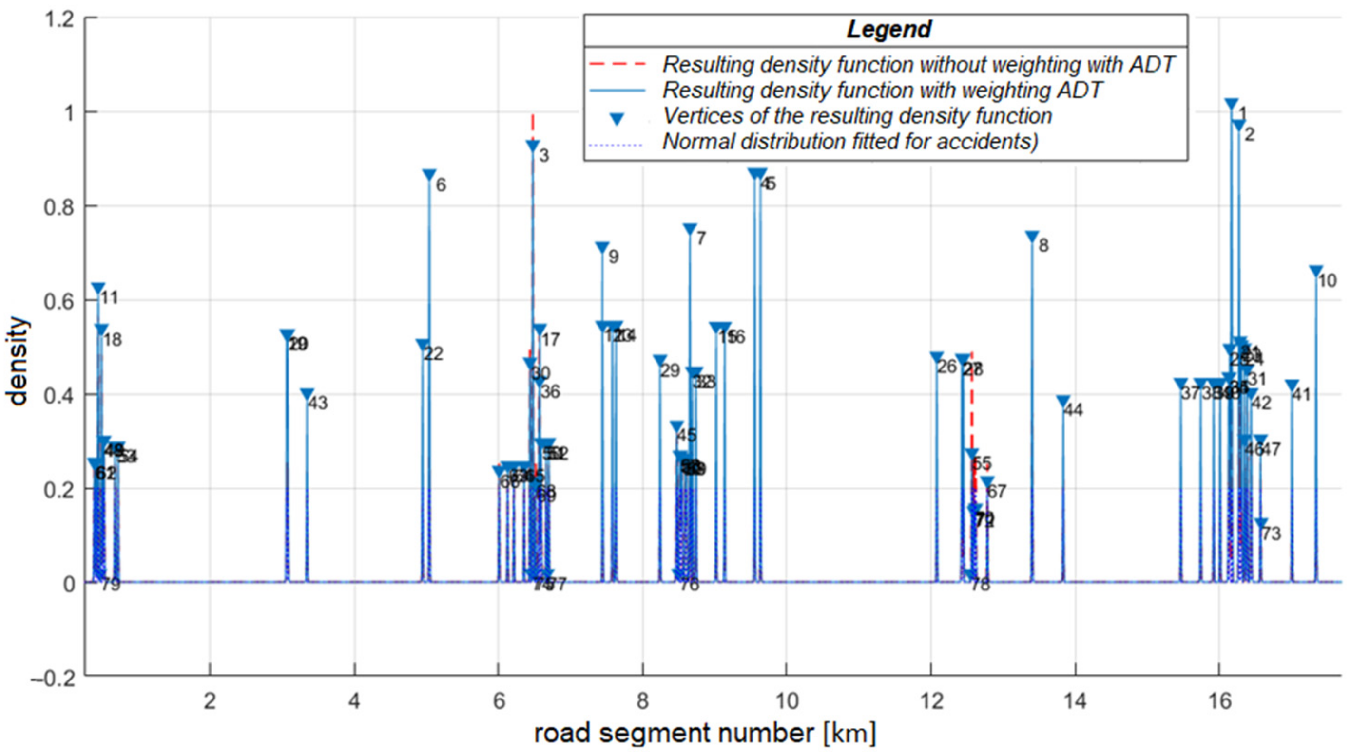
According to the cross-sectional traffic count, the annual average daily traffic is the volume of traffic per vehicle/day for the examined route section (which is the annual average of the daily traffic passing through the cross-section of the road). The AADT was determined on the basis of validity sections. A validity section is a section between two measuring stations, where the AADT is regarded as constant. Because of the nodes, there are jumps in the function as there is a change in the traffic. The value of the total kernel was weighted by the AADT because the cyclist accident risk is higher if there is more car traffic. Thus, we weighted our resulting density function with the annual average daily traffic for the given section (
Figure 3).
The x-axis of the coordinate system represents the road segment numbers, and the y-axis shows the value of the resulting density function. Because of the low-prefix y values, we have normalized them from 0 to 1 for the sake of visualization and simplicity.
The normal distributions of accidents are shown with dotted blue lines. The resulting density function weighted by annual average daily traffic (AADT) is denoted by the solid blue line, while the one without AADT is shown by the dashed red line. The triangles with numbers denote the vertices of the resulting density function according to the descending order of
y. We examined whether weighted and non-weighted black spots follow the same distribution. Because the data sets do not follow a normal distribution, only non-parametric tests can be considered. Our sample was paired, so only the Wilcoxon test was accepted [
38]. The essence of this is that if the two paired samples are from the same distribution, then the sum of the positive differences between the two samples follows a normal distribution with a predetermined expected value and standard deviation. In our case, the null hypothesis, i.e., that the two samples follow the same distribution, can be rejected. Thus, it can be clearly demonstrated that the introduction of AADT significantly influences the outcome of focal research.
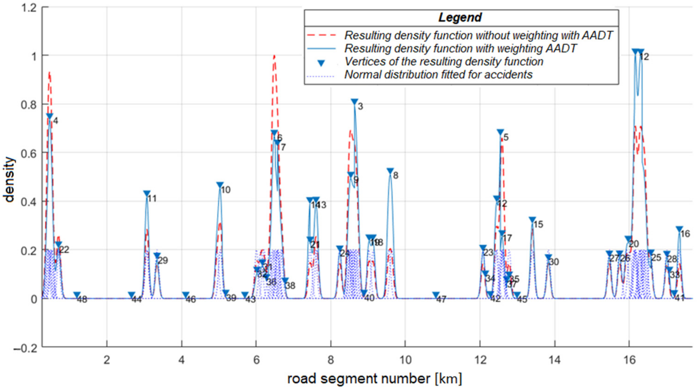
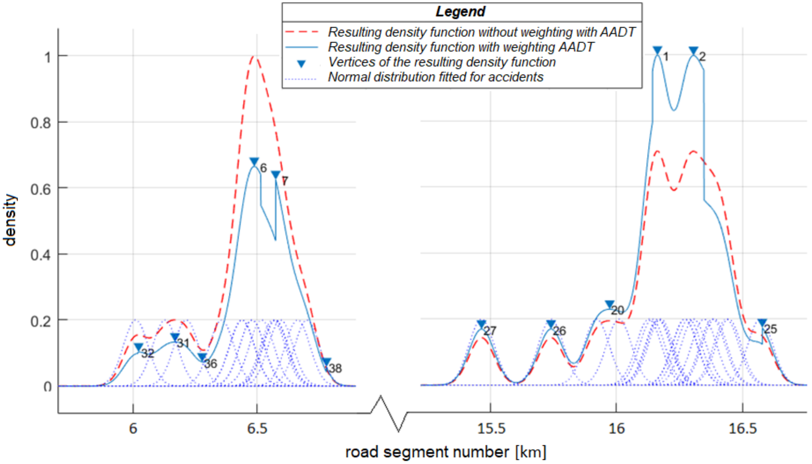
In
Figure 4, the difference between the weighted and non-weighted density functions can be observed. In the left section of the diagram, we can see that only one vertex was formed in the non-weighted case (dashed red curve), and two vertices were formed in the weighted case (triangles). Besides, the former one took a higher value. The diagram section on the right is a counterexample to the previous one. In this case, the AADT weighted function shows a higher value. Although the same number of accidents occurred in both places, the comparison of the two shows that in the left side case, the annual average daily traffic was higher than in the right-side case. This example illustrates why weighting with annual average daily traffic is essential. Significant differences may arise between the cases weighted and unweighted with annual average daily traffic.
In the case of equal accident frequency, the accident density is low in the case of high traffic, and high in the case of low traffic, it is needed to include the traffic intensity parameter into the model so that critical sections can be detected properly.
3.2. Determining the Starting Points and Endpoints of the Accident Black-Spots
The question arises as to which points of our resulting accident density are to be called accident black spots, i.e., how they are defined. The optimal solution proved to be to filter out the statistically significant outliers from the density function for each segment number (per meter). These values represent our accident black spots. In our formulation, we refer to values that are above the 75% percentile and interquartile range with at least one and a half times as outliers. By declaring this value, the starting points and endpoints of our accident black-spots can be determined [
39,
40,
41]. Therefore, in theory, we can draw a horizontal line at this
y value. The intersections of this line and our resulting kernel function determine the starting points and endpoints of our accident black spots.
3.3. Accident Concentration Sites on the Main Road No. 1
This novel mathematical algorithm was applied to data for the main road No. 1 in Hungary, and then the outliers were used to determine the starting points and endpoints of our accident black spots, as shown in
Table 3.
Altogether, 11 sections of the main road No. 1 that represent a potential danger to cyclists and pedestrians have been identified by using the novel methodology, i.e., by applying the kernel density estimation method and by detecting accident black spots with the outliers. Contrary to this, three black spots could be defined by using the distance matrix method [
5].
Table 3 reveals the difference between the results of the two distinct methodologies. Based on the new KDE with AADT Method, more black spots can be identified in a more accurate way.
4. Discussion
4.1. Applicability of the Kernel Density Estimation Method
Unlike our distance matrix method, our kernel-based density estimation algorithm is based on non-fixed length segments. The starting points and endpoints of our accident black spots were greatly influenced by the location of the accidents on the road and the annual average daily traffic. The Win-Bal accident database management program would encode not only the number of the road on which the accident occurred but also the number of the crossing road, if there were any. This information could also be taken into account in our kernel-density-based estimation method. Hence, if the number of the crossing road was identical to the number of the road we were investigating, then that accident was also included in the accidents on the road under investigation. In this way, we could also take into account accidents that occurred on the other road connected to the road under investigation, but the road under investigation may have had an impact on the occurrence of the accident.
In terms of sections with the same accident frequency, the accident density turns low at high traffic volume, and it is high at low traffic volume. Consequently, integrating the traffic volume into the model is crucial. Thus, our kernel-based accident density locator algorithm takes into account the annual average daily traffic to ensure that the results are even more accurate.
In our previous research [
5], we examined the autoregressive integrated moving average method (Moving Window Method), and we developed a distance matrix road accident black spot search algorithm as well. In order to prevent errors in those methods, we created an algorithm based on kernel density estimation. The three methods are compared in
Figure 5. Cells with a green background indicate the advantages, and the cells with a red background show the disadvantages compared to the other methods.
In statistics, the problem of histogram creation is well-known, and it is also a major drawback of the Moving Window Method or the distance matrix method. The process is sensitive to the width of intervals and also the starting point of intervals. Furthermore, in the Moving Window Method applied for road accident analyses, it is not easy to determine the limit above which a certain place is considered a black spot. Due to these problems, some places are identified as black spots erroneously, while some real black spots might remain undetected. Thus, the identification of true intervention points is not satisfactory.
The kernel method offers a solution to the above problems. This method calculates a given distribution for each accident, and these distributions are summed. The resultant density function is then analyzed statistically to identify the limits above which values count as outliers even in the statistical sense. Consequently, the real black spots can be analyzed without including a subjective evaluation technique in the system.
4.2. Sensitivity Analysis—The Selection of the Kernel
According to
Table 2, there is no significant difference in the efficiency of the tested kernels. This stability is supported by the following figure, which depicts the resulting density function of accidents on the main road No. 1. It can be seen that the four kinds of distributions closely follow each other, so using any of them (normal, Epanechnikov, box, triangle) would yield very similar values (
Figure 6). The selection of the normal kernel function was justified by a special case. In Hungary, the locations of accidents are recorded by the police by means of digital tools, so the GPS coordinates underlying the analysis are accurate and reliable. We analyzed the distribution of distances between the recorded GPS coordinates and the endpoints of the whole accident sections on a partial sample. The normality analysis of the samples (the distances [m] between the GPS coordinate pairs and accident sections) was conducted by the Shapiro–Wilks Test [
42]. As the result of this test, the normality could be confirmed, so we selected the normal kernel accordingly.
4.3. Sensitivity Analysis—Determination of Bandwidth
Unlike the histogram, the kernel density estimation yields a smooth estimate. The smoothness can be set up by using the kernel bandwidth parameter. By choosing the right bandwidth, essential characteristics of the distribution can be observed, while poor choice may result in over-smoothed or under-smoothed and hidden functions [
43].
We have tested our algorithm with multiple bandwidths. The following two figures illustrate extreme cases. These show how too low or too high bandwidths affect the kernel function.
In
Figure 7, bandwidth 50 is depicted. It can be observed that a low number of kernel functions overlap. Therefore, these functions do not add up, so an under-smoothed kernel is created. In contrast,
Figure 8 illustrates the bandwidth 5000 cases. Due to the too high bandwidth, the kernel functions overlap largely, as a result of which the resulting density function will be over-smoothed. On the curve weighted by annual average daily traffic, which is indicated by a continuous line, sharp jumps are caused by the change in the annual average daily traffic. Based on our over-smoothed and under-smoothed investigations and the international literature [
8], we have finally chosen 300 as the bandwidth in order to specify the critical locations where the density of road traffic accidents is explicitly high.
It can be stated that the proper selection of the bandwidth is essential if the kernel density estimation is used. In the case of a few tens of meters of bandwidth, only accidents which are close to each other in space are added up. In the case of a few thousands of meters of bandwidth, also the kernel function of those accidents could overlap which are far away from each other and happened under completely different infrastructural conditions. In the latter case, the length of the accident concentration sites can be so considerable that in the course of our further research, we would not be able to define the typical infrastructure characteristics of the sections.
Different bandwidths are used when examining different areas of life. For traffic accidents, we recommend a few hundreds of meters of bandwidth. It provides an optimal solution in which those accidents close to each other are added up, which are located on road sections with similar infrastructure, and thus, the conditions that lead to accidents can be explored later.
5. Conclusions
This study only dealt with road accidents in Hungary in which a pedestrian and/or cyclist was affected. A normal distributed kernel function was fitted to every accident, and then the cumulative density function was created as the weighted sum of these kernels.
The efficiency of kernel functions was demonstrated, and it was shown how their bandwidth affects the result and under which conditions they may be used in the analysis of road traffic accidents. It turns out that there is no significant difference in the efficiency of the tested kernels. However, the right selection of bandwidth dramatically influences the result. With the example of accidents occurring on the road No. 1, it was illustrated when a resultant density function can be considered as over-smoothed or under-smoothed.
The resultant density function was analyzed both with weighted annual average daily traffic and without that. It was concluded that the latter case significantly distorts the results because it is essential to consider whether a certain number of accidents occurred at low or high AADT. The main advantage of this method is that all the black spots can be identified with the goal of preventing future accidents. The most critical locations must be chosen so that we can create the optimal ranking of investments.
It was an important issue to detect which points of the resultant density function are called accident concentration sites. For this purpose, we used the percentile values and the interquartile range used in the descriptive statistics. Based on the method proposed in this article, the outliers of the resultant density function were specified, with the help of which the accident concentration sites could be identified. Accidents occurring on road No. 1 in Hungary were used as an example to demonstrate under which conditions the method is applicable in analyzing pedestrian and cyclist accidents.
As a continuation of the research, we would like to run our method on all primary and secondary roads in Hungary. This way, we would get a comprehensive nationwide pedestrian and bicycle accident black-spot map. After that, we would like to examine these accident sites in order to determine the cause of the increase in accidents and propose changes to the authorities.
In order to reduce the number of road accidents, in addition as in addition to proactive methods, reactive approaches, such as black-spot identification methods, are also required, which can only be applied on a reliable mathematical-statistical basis. The result of black-spot identification determines the sites for traffic-related investments and affects investment priority ranks. Consequently, the constant development of these methodologies is justified and necessary so that the methods can determine which sections of the public road network have a potentially high risk of accidents as accurately as possible.
Author Contributions
Conceptualization, D.B. and T.S.; methodology, D.B. and T.S.; software, D.B. and T.S.; formal analysis, D.B.; resources, T.S.; writing—original draft preparation, D.B. and T.S.; writing—review and editing, D.B. and T.S.; visualization, D.B.; supervision, T.S. All authors have read and agreed to the published version of the manuscript.
Funding
This research was funded by OTKA, grant number OTKA-K-134760.
Institutional Review Board Statement
Not applicable.
Informed Consent Statement
Not applicable.
Data Availability Statement
Restrictions apply to the availability of these data. Data was obtained from KTI Institute for Transport Sciences and are available from the authors with the permission of KTI Institute for Transport Sciences.
Acknowledgments
Authors are greatly acknowledging the support of OTKA-K-134760 supervised by Adam TOROK.
Conflicts of Interest
The authors declare no conflict of interest.
References
- Sokolovskij, E.; Prentkovskis, O. Investigating traffic accidents: The interaction between a motor vehicle and a pedestrian. Transport 2013, 28, 302–312. [Google Scholar] [CrossRef]
- Baranyai, D.; Levulyté, L.; Török, Á. Vulnerable road users in Hungary. In Proceedings of the 20th International Scientific Conference Transport Means, Juodkrante, Lithuania, 5–7 October 2016; pp. 1126–1130. [Google Scholar]
- Jonas, M.; Jurijus, Z.; Robertas, P. Analysis of the influence of fatigue on passenger transport drivers’ performance capacity. Transport 2012, 27, 351–356. [Google Scholar] [CrossRef]
- Madleňák, R.; Madleňáková, L.; Hoštáková, D.; Drozdziel, P.; Török, A. The analysis of the traffic signs visibility during night driving. Adv. Sci. Technol. 2018, 12, 71–76. [Google Scholar] [CrossRef]
- Baranyai, D.; Török, Á. Analysing the pedestrian and bicycling traffic in Hungary with the method of the distant matrix. In Proceedings of the Road Accidents Prevention Conference, Novi Sad, Serbia, 13–14 November 2016; pp. 11–14. [Google Scholar]
- Sokolovskij, E. Automobile braking and traction characteristics on the different road surfaces. Transport 2007, 22, 275–278. [Google Scholar] [CrossRef] [Green Version]
- Banos, A.; Huguenin-Richard, F. Spatial distribution of road accidents in the vicinity of point sources application to child pedestrian accidents. Geogr. Med. 2000, 8, 54–64. [Google Scholar]
- Sedoník, J.; Bíl, M.; Andrásik, R.; Svoboda, T. The KDE+ software: A tool for effective identification and ranking of animal-vehicle collision hotspots along networks. Landsc. Ecol. 2015, 31, 231–237. [Google Scholar] [CrossRef]
- Pulugurtha, S.S.; Krishnakumar, V.K.; Nambisan, S.S. New methods to identify and rank high pedestrian crash zones: An illustration. Accid. Anal. Prev. 2007, 39, 800–811. [Google Scholar] [CrossRef]
- Blazquez, C.A.; Celis, M.S. A spatial and temporal analysis of child pedestrian crashes in Santiago, Chile. Accid. Anal. Prev. 2013, 50, 304–311. [Google Scholar] [CrossRef]
- Guler, Y.; Sebnem, D. Spatial analysis of two-wheeled vehicles traffic crashes: Osmaniye in Turkey. KSCE J. Civ. Eng. 2015, 19, 2225–2232. [Google Scholar] [CrossRef]
- Yunxuan, L.; Mohamed, A.; Jinghui, Y.; Zeyang, C.; Jian, L. Analyzing traffic violation behavior at urban intersections: A spatiotemporal kernel density estimation approach using automated enforcement system data. Accid. Anal. Prev. 2020, 141, 105509. [Google Scholar] [CrossRef]
- Anderson, T.K. Kernel density estimation and K-means clustering to profile road accident hotspots. Accid. Anal. Prev. 2009, 41, 359–364. [Google Scholar] [CrossRef] [PubMed]
- Hashimoto, S.; Yoshiki, S.; Saeki, R.; Mimura, Y.; Ando, R.; Nanba, S. Development and application of traffic accident density estimation models using kernel density estimation. J. Traffic Transp. Eng. Engl. Ed. 2016, 3, 262–270. [Google Scholar] [CrossRef] [Green Version]
- Andrásik, R.; Bíl, M. Traffic accidents: Random or pattern occurrence? In Safety and Reliability of Complex Engineered Systems; Luca, P., Bruno, S., Bozidar, S., Enrico, Z., Wolfgang, K., Eds.; Taylor & Francis Group: London, UK, 2015; pp. 3–6. [Google Scholar] [CrossRef]
- Bíl, M.; Andrásik, R.; Janoska, Z. Identification of hazardous road locations of traffic accidents by means of kernel density estimation and cluster significance evaluation. Accid. Anal. Prev. 2013, 55, 265–273. [Google Scholar] [CrossRef]
- Álvaro, B.; Francisco, M.; Francisco, M. Spatial analysis of traffic accidents near and between road intersections in a directed linear network. Accid. Anal. Prev. 2019, 132, 105252. [Google Scholar] [CrossRef]
- Erdogan, S.; Yilmaz, I.; Baybura, T.; Gullu, M. Geographical information systems aided traffic accident analysis system case study: City of Afyonkarahisar. Accid. Anal. Prev. 2008, 40, 174–181. [Google Scholar] [CrossRef]
- Matthias, J.K.; Durot, S. Segmentation of lines based on point densities—An optimisation of wildlife warning sign placement in southern Finland. Accid. Anal. Prev. 2006, 39, 38–46. [Google Scholar] [CrossRef]
- Prasannakumar, V.; Vijith, H.; Charutha, R.; Geetha, N. Spatio-Temporal Clustering of Road Accidents: GIS Based Analysis and Assessment. Procedia Soc. Behav. Sci. 2011, 21, 317–325. [Google Scholar] [CrossRef] [Green Version]
- Mamoudou, S.; Sharut, G.; Samia, B.; Soumya, B.; Paul, M. Exploring the forecasting approach for road accidents: Analytical measures with hybrid machine learning. Expert Syst. Appl. 2021, 167, 113855. [Google Scholar] [CrossRef]
- Zhixiao, X.; Jun, Y. Kernel Density Estimation of traffic accidents in a network space. Comput. Environ. Urban Syst. 2008, 32, 396–406. [Google Scholar] [CrossRef] [Green Version]
- Zhixiao, X.; Jun, Y. Detecting traffic accident clusters with network kernel density estimation and local spatial statistics: An integrated approach. J. Transp. Geogr. 2013, 31, 64–71. [Google Scholar] [CrossRef]
- Steenberghen, T.; Dufays, T.; Thomas, I.; Flahaut, B. Intra-urban location and clustering of road accidents using GIS: A Belgian example. Int. J. Geogr. Inf. Sci. 2004, 18, 169–181. [Google Scholar] [CrossRef]
- Utoyo, B.; Agus, P.S. Traffic accident blackspot identification and ambulance fastest route mobilization process for the city of Surakarta. J. Transp. 2012, 12, 237–248. [Google Scholar]
- Liljana, Ç.; Shino, S.; Krsto, L. Integrating GIS and spatial analytical techniques in an analysis of road traffic accidents in Serbia. Int. J. Traffic Transp. Eng. 2013, 3, 1–15. [Google Scholar] [CrossRef]
- Van der Walt, C.M.; Barnard, E. Variable kernel density estimation in high-dimensional feature spaces. In Proceedings of the Thirty-First AAAI Conference on Artificial Intelligence (AAAI-17), San Francisco, CA, USA, 4–9 February 2017. [Google Scholar]
- Moslem, S.; Gul, M.; Farooq, D.; Celik, E.; Ghorbanzadeh, O.; Blaschke, T. An integrated approach of best-worst method (BWM) and triangular fuzzy sets for evaluating driver behavior factors related to road safety. Mathematics 2020, 8, 414. [Google Scholar] [CrossRef] [Green Version]
- Silverman, B.W. Density estimation for statistics and data analysis. In Monographs on Statistics and Applied Probability; Chapman and Hall: London, UK, 1986. [Google Scholar]
- Correa-Quezada, R.; Cueva-Rodríguez, L.; Álvarez-García, J.; Río-Rama, M.D.L.C.D. Application of the Kernel Density Function for the Analysis of Regional Growth and Convergence in the Service Sector through Productivity. Mathematics 2020, 8, 1234. [Google Scholar] [CrossRef]
- Hamar, D. Applying and Comparing Kernel-Based Estimators for Function Approximations. In Hungarian: Magfüggvényes Becslés Alkalmazása és Összehasonlítása Függvény-Közelítések Esetén. Bachelor’s Thesis, University of Miskolc, Miskolc, Hungary, 2014. [Google Scholar]
- Pauer, G.; Török, Á. Comparing System Optimum-based and User Decision-based Traffic Models in an Autonomous Transport System. Promet-Traffic Transp. 2019, 31, 581–591. [Google Scholar] [CrossRef]
- Fatima, Z.L.; Abderrahmane, B.; Amine, B.C.; Khaled, Z.; Svetlin, G. Density Problem some of the Functional Spaces for Studying Dynamic Equations on Time Scales. J. Sib. Fed. Univ. Math. Phys. 2022, 15, 46–55. [Google Scholar] [CrossRef]
- Van der Walt, C.M. Maximum-Likelihood Kernel Density Estimation in High-Dimensional Feature Spaces. Ph.D. Thesis, Department of Information Technology Faculty of Economic Sciences, North-West University, Potchefstroom, South Africa, 2015; pp. 20–21. [Google Scholar]
- Khaled, Z. Stabilization for solutions of plate equation with time-varying delay and weak-viscoelasticity in ℝn. Russ. Math. 2020, 64, 21–33. [Google Scholar] [CrossRef]
- Khaled, Z.; Tosiya, M. Lifespan of solutions for a class of pseudo-parabolic equation with weak-memory. Alex. Eng. J. 2020, 59, 957–964. [Google Scholar] [CrossRef]
- Bouchra, A.; Brahim, T.; Khaled, Z. Positive solutions for integral nonlinear boundary value problem in fractional Sobolev spaces. Math. Methods Appl. Sci. 2021, 1–17. [Google Scholar] [CrossRef]
- Wilcoxon, F. Individual Comparisons by Ranking Methods. Biom. Bull. 1945, 1, 80–83. [Google Scholar] [CrossRef]
- Ferreira, J.E.V.; Pinheiro, M.T.S.; dos Santos, W.R.S.; Maia, R.D.S. Graphical representation of chemical periodicity of main elements through boxplot. Educ. Química 2016, 27, 209–216. [Google Scholar] [CrossRef] [Green Version]
- Ghadi, M.; Török, Á. A comparative analysis of black spot identification methods and road accident segmentation methods. Accid. Anal. Prev. 2019, 128, 1–7. [Google Scholar] [CrossRef] [PubMed]
- Sipos, T. Spatial Statistical Analysis of the Traffic Accidents. Period. Polytech. Transp. Eng. 2017, 45, 101–105. [Google Scholar] [CrossRef] [Green Version]
- Shapiro, S.S.; Wilk, M.B. An Analysis of Variance Test for Normality (Complete Samples). Biometrika 1965, 52, 591–611. [Google Scholar] [CrossRef]
- Shi, Y.; Lv, L.; Yu, H.; Yu, L.; Zhang, Z. A Center-Rule-Based Neighborhood Search Algorithm for Roadside Units Deployment in Emergency Scenarios. Mathematics 2020, 8, 1734. [Google Scholar] [CrossRef]
| Publisher’s Note: MDPI stays neutral with regard to jurisdictional claims in published maps and institutional affiliations. |
© 2022 by the authors. Licensee MDPI, Basel, Switzerland. This article is an open access article distributed under the terms and conditions of the Creative Commons Attribution (CC BY) license (https://creativecommons.org/licenses/by/4.0/).


