1. Introduction
Today, it is becoming increasingly important to correctly plan tourism development strategy, as the global tourism market is recovering from the shock of the COVID-19 pandemic. Correct forecasting and rational planning of tourism development can be a crucial factor in providing a decisive advantage in the global tourism market. Taking into account the impact of major factors is a fundamental condition in planning future tourism development.
Uzbekistan is located at the crossroads of the ancient Silk Road, which has attracted thousands of traders and invaders throughout the centuries. Because of its strategic location, it was the center of events between Russia and Great Britain later referred to as the Great Game. There are many fascinating historical sites and attractive exotic places to visit in the heart of Central Asia. Thus, in theory, Uzbekistan has great advantages with regard to becoming a new mainstream tourism destination. However, the tourism infrastructure is not developed in many parts of the country, and there may be many other factors that prevent Uzbekistan from becoming major world tourism attraction [
1]. Nevertheless, government is taking measures to support investors in building infrastructure, thereby contributing to the development of domestic tourism, which is crucial in the progress of overall tourism. In our view, if the country develops a reasonable plan of tourism development then it has a chance to change the balance of power in the competition for global tourist inflows.
With the emergence of COVID-19 in 2020, tourism and the travel sector faced unprecedented challenges. Uzbekistan’s tourism sector was hit by the effect of strict quarantines, when the whole tourism sphere was essentially frozen. The measures taken by government to support the economy included creating a USD 1 billion Anti-Crisis Fund, which made it possible to lengthen the tax-free period for travel companies and tourism infrastructure. Moreover, the state expanded funding healthcare, covered the cost of quarantines and salary supplements for healthcare workers, assisted affected businesses via subsidies, created additional public works, and extended a moratorium on tax audits as well as delaying tax declarations [
2]. Taking these measures enabled the republic to maintain its key tourism infrastructure facilities in working condition.
In this study, we tried to take into account the impact of the environment, which shapes the suitable conditions for humans, flora, and fauna to exist [
3]. One of the most promising tourism types is ecotourism, where people travel to learn about biodiversity in various habitats [
4]. Such activities are becoming more and more popular among younger generations as their average income rises [
5]. Therefore, in order to stimulate higher tourism demand and ensure competitiveness, it is becoming important to apply innovational technologies that enable remote visualization of all the features of a particular eco-zone [
6]. However, it is crucial to minimize the negative impact of over-tourism on natural habitats [
7,
8].
The main purpose of the present research is to assess the impact of factors such as welfare, infrastructure, security level, and the environment on inbound tourism. Today, a high security level in a tourism destination has become one of the main preconditions for attracting tourists in the post-pandemic world. The results of previous research confirm the significance of security in the development of inbound tourism.
According to Dwyer, L. and Forsyth, P., the domestic output (level of consumption) is a major factor that drives inbound tourism [
9]. In this article, we tried to assess the short- and long-term effect of real GDP per capita, which can represent the level of consumption and welfare, on the inbound tourism using the ARDL model. In addition, we forecast inbound tourism demand using the ARIMA model, which showed that the COVID-19 pandemic will continue to exert a negative effect for more than five years. Our study stands out from similar researches on inbound tourism demand by focusing on assessing the impact of factors which shape destination competitiveness on inbound tourism, with extensive empirical analysis using the example of Republic of Uzbekistan. Previous studies rarely used macroeconomic data to assess the inbound tourism demand of Uzbekistan; rather, the priority was on survey analysis [
10]. Allaberganov and Preko [
10], in their research, found a positive correlation between travel motives and the frequency of visitation of international tourists to Uzbekistan. They used survey data from 563 international tourists; in other words, it was static data taken only for one period. However, it is crucial to estimate the impact of various factors on inbound tourism using dynamic data. Our research partially fills this gap by using data from 21 time series as well as econometric models to assess the impact of four crucial factors on inbound tourism. The purpose of this research was to explore macro-level data that was related to constructing a tourism development strategy able to boost the country’s competitiveness as a tourism destination. At the end of the day, we are able to state that all of the reported results obtained in this research were statistically significant and can be applied in practice. The statistical data used for analysis were taken from the official website of Department of Statistics of Uzbekistan. These research results can be used by regional governing bodies for the strategic planning of tourism development.
2. Literature Review
The use of economic and mathematical methods makes it possible to conduct a qualitative and quantitative analysis of economic phenomena in order to provide a quantitative assessment of the significance of risk and market uncertainty and choose an effective solution.
According to [
11], three main methods based on empirical studies of tourism forecasting can be distinguished, namely, causal models (econometric or spatial models), time series models, and various qualitative models. Goh and Law [
12] identify three types of quantitative forecasting methods: time series models, econometric models, and AI-based models. Time series models require only one data series, where past data is extrapolated into the future patterns. Even though time series models are widely used, these models are hard to interpret as they are not based on any economic theory. Time series models are divided into simple (simple moving average, single exponential smoothing) and advanced (double exponential smoothing, autoregressive moving average, simple structural time series) subcategories.
Peng et al. [
13] emphasize the use of econometric models for determining the causality structure and evaluate the influence of different variables on future tourism demand. To put it simply, the aim of econometric methods is not extrapolation, it is identifying the group of explanatory factors [
14]. Simple regression, gravity models, vector autoregression, error correction models, cointegration, and autoregressive distributed lag models are common types of econometric models [
12].
From the beginning of the 2000s models based on artificial intelligence have been used for forecasting purposes in various fields [
15]. AI-based models such as artificial neural networks, support vector machines, fuzzy time series, genetic algorithms, and expert systems have proven to be more effective than traditional forecasting methods [
16]. Even though the forecasted values seem to be more accurate for AI-based models, it is hard to identify the path taken by the learning process, which is based on adjusting weights of respective neurons (nodes) via synapses [
15]. Therefore, AI-based models are usually used with big data, where classification or identification of clusters has greater priority. Identifying clusters can be important in forming hypotheses, which can then be verified by econometric methods. Nowadays many researchers use various forecasting methods in combination in order to reach research goals [
17].
The research of Dwyer and Forsyth on assessing inbound tourism is the most notorious and extensive work on the analysis of inbound tourism demand. In their research, they point out domestic consumption as the strongest factor driving tourism demand upwards [
9]. Milenkovski et al. [
18] analyzed the impact of traffic infrastructure on the inbound tourism in the Republic of Macedonia. They assert the critical impact of security and environment of inbound tourism. In their research, Breda et al. [
19] studied the impact of safety and security measures on inbound tourism in China. Their research results show that political and social stability, security, and fashion trends significantly affected inbound tourism demand. Moreover, they point out the impact of outbreaks on structural changes in Chinese tourist agencies. However, the research conducted by Biagi et al. [
20] showed that crime could be positively correlated with tourism. According to Sunlu [
21], tourism might negatively impact the environment when the number of visitors is greater than the capacity of the tourism destination. Among the potential negative impacts he lists air, water, and land pollution as well as other physical impacts on the ecosystem of a destination. However, surprisingly few studies have focused on assessing the impact of the four above-mentioned group factors on inbound tourism. Our research is an empirical experiment that might add value to fill this research gap.
3. Working Methodology
3.1. General Overview of Forecasting Methodology
Forecast indicators use factographic, expert, and mixed methods, depending on the nature of the data obtained. Factographic methods are based on actual data from the past and represent the current development forecast of the object. Essentially, this method is widely used in the analysis of processes of an evolutionary nature. Expert (intuitive) methods are used by qualified experts to calculate future values by summarizing their opinions about the object of forecasting. The expert method is widely used in many ways to predict structural changes and processes leading to radical change. Mixed methods mainly use real or expert data as initial data. In turn, each method is divided into groups and subgroups. For example, factographic methods are divided into statistical and advanced methods [
13].
Forecasting methods can be divided into two large groups. Logical-heuristic methods are based on the well-known general scientific theory of logic and on heuristics, which is defined by dictionaries as “the art of finding the truth”.
Modeling methods, on the other hand, are based primarily on quantitative, mathematical, and statistical studies on the identification of formal dependencies and development trends, the construction of predictive models, and experimenting with them on the basis of computer technology. As subclasses, extrapolation models, econometric, normative-target, and simulation models can be distinguished [
22]. Separately, this classification presents complex methods in which both logical-heuristic approaches and modeling are composed [
23].
3.2. Overview of Uzbekistan’s Inbound Tourism Statistics
According to the State Committee of Statistics, the dynamics of foreign citizens visiting the Republic of Uzbekistan increased significantly from 2017 to 2019. This number was 2.6 million in 2017, 6.4 million in 2018, and 8.3 million in 2019, an increase of 2.9 times over the same period. The largest number of foreigners visiting the country was from the following countries: Kazakhstan—2456.9 thousand people (29.6% of the total number of visitors); Tajikistan—2389.4 (28.8%); Kyrgyzstan—1533.6 (18.4%); and Russia—592.4 (7.1%). The largest influx from far abroad was from: Turkey—107.9 thousand people (1.3%); China—61.8 (0.7%); South Korea—40.6 (0.5%); India—32 thousand people (0.3%); Germany—28.9 (0.3%); and Japan—25.2 thousand people (0.3%). However, the COVID-19 pandemic negatively affected inflow, resulting in a decrease of almost 76% in 2020 relatively to 2019.
The age distribution of citizens entering the Republic of Uzbekistan in 2019 was as follows: the majority were 31–55 years old (53.1%); 19–30 years old—21.8%; and 55 years old and older—17.3%. Outflow of citizens of Uzbekistan to the CIS countries in 2019 amounted to 12,402.05 thousand people, which is 96% of the total number of migrants, of which the number of emigrants to foreign countries was 530.6 thousand people (4%). The main part of people of the Republic of Uzbekistan going abroad visit the CIS countries: (51.6%) visit the Republic of Kazakhstan (7139.8 thousand people); Kyrgyzstan—23.1% (3196.8 thousand people); and the Russian Federation—1178.7 thousand people (8.5%). In terms of far abroad countries, the main outflow was South Korea (79.7 thousand people), along with China, the United States, Germany and others.
A comparative analysis of the number of tourist visits in the world shows that the visits were made mainly for tourism and leisure purposes. In Russia and Uzbekistan, such tourist visits account for 10% and 7.1%, respectively.
The analysis of the current state of tourism in the Republic of Uzbekistan shows that in recent years this sector has been developing steadily and rapidly. In particular, annual growth in the rate of domestic tourist flow has been observed. The sharp increase in demand for tourist services in the country has led to the construction of international-class hotels in resort areas, mainly in Tashkent, Samarkand, Bukhara, and other large cities, contributing to the formation of a chain of hotels in the country.
Over the past five years, the number of companies and organizations engaged in tourism has increased. For example, their number in 2012 was 345. There were 68 (13.2%) tourist organizations and 31.4 thousand foreign tourists in the Samarkand region, 37 tourist organizations and 3.7 thousand foreign tourists in the Bukhara region, and 11 tourist organizations and 177.3 thousand foreign tourists in the Khorezm region. In 2019, 64.2% of companies engaged in tourism were located in Tashkent, 13.2% in Samarkand, 7.1% in Bukhara, and 2.1% in Khorezm.
3.3. Specific Methodology Application
We decided to examine the statistics of inbound tourism, as this indicator is important in assessing the overall tourism demand in any tourism destination. In order to have a clear idea of the principles, methods, and means of improving and ensuring the quality of the tourism network, it is necessary to identify key factors that may change the description and characteristics of the proposed tourism product. By tourism product, we mean tangible products that tourists buy, as well as intangible services that are consumed by particular segment of tourists. In Uzbekistan, the largest share of tourism product segmentation consists of historical sightseeing trips (90%) [
24]. Most tourists’ age ranges from 30 to 45 years (75%) [
24]. Income from domestic tourism constitutes about 80% of total tourism income in Uzbekistan [
24].
In order to estimate the impact of factors on inbound tourism, we used an ordinary least squares multiple regression model. Our aim was to assess the impact of welfare, infrastructure, security level, and the environment on inbound tourism. For this reason, we chose proxies of the above-mentioned categories, namely, welfare (life expectancy, consumer price index, real GDP per capita), infrastructure (passenger transportation volume), environment (CO2 emissions), and security level (total crimes recorded).
One of the most popular forecasting methods is the Box Jenkins methodology [
25]. Technically, this method is called the ARIMA model. According to [
13], ARIMA is one of the most accurate for seasonal data. However, the overall performance of ARIMA models does not always lead to the conclusion that sophisticated methods are better than simpler ones [
13]. We used the ARIMA model to forecast the number of inbound tourists arriving in the Republic of Uzbekistan.
Before considering the prerequisites for regression analysis, it should be said that the general condition for obtaining more stable results when constructing OLS regression models of the volume of inbound tourism is a requirement for the homogeneity of the initial information [
26,
27]. This information must be processed for anomalous observations, i.e., those sharply distinguished from the array of data. This procedure is performed by quantifying the homogeneity of the population according to certain one-dimensional or multidimensional criteria (depending on the initial information) and aiming at those objects of observation that have the best (or worst) conditions for functioning for independent or weakly dependent reasons [
28]. After processing the data for anomalies, the extent to which the remaining information satisfies the prerequisites for using a static apparatus in building models must be checked, as even slight deviations from these prerequisites often nullify the obtained effect [
29]. It should be borne in mind that a probabilistic or statistical solution of any economic problem should be based on a detailed understanding of the initial mathematical concepts and premises and the correctness and objectivity of the collection of initial information [
30] in constant combination with the tightness of the relationship between economic and mathematical–statistical analysis.
In order to apply regression analysis, it is necessary that all the variables under consideration be random and have a normal distribution law. Moreover, the fulfillment of these conditions is necessary only for a probabilistic assessment of the revealed tightness of the connection.
The least squares method can be used when a model that serves to represent a problem is represented as a system of equations by means of several production functions. However, the calculation of parameter values for a system of equations has certain peculiarities [
31]. Most important is that the system of equations is characteristic in terms of quantity and the location of variables in the equation [
32].
A number of government decisions and programs have been adopted to increase the flow of tourists to the country, to make entry and domestic tourism the most important sector of the economy, and to promote the cultural and historical heritage and natural resources of the country. The measures taken by the government were marked by the role of inbound and domestic tourism as a source of free currency conversion and an important reserve to replenish the GDP.
4. Materials and Methods
In our study, we used the STATA 14 and EVIEWS 10 statistical packages to analyze the data shown in
Table 1. We selected factors representing the welfare (GDP per capita, life expectancy, consumer price index), infrastructure (passenger transportation volume, million people), security level (total crime records, units), and environmental impact (CO
2 emissions, metric tons per capita). The data below represent the dynamics of the above-mentioned factors from 2000 to 2020.
The aim of our analysis was to identify the impact of the welfare, security, and environmental factor groups on the aggregate inbound tourism demand.
Linear regression analysis consists of fitting a graph for a set of observations using the least squares method. Regression is used to analyze the impact of the values of one or more independent variables on a single dependent variable. The first step in any regression analysis is analyzing the structure of the dependent and independent variables. Below, the descriptive statistics of the analyzed dataset are provided (
Table 2). It is clear from
Table 2 that for certain variables, such as real GDP per capita, the number of inbound tourists have large variation, as their minimum and maximum value range widely. However, this is not good for time series analysis, as it is clear that both of these variables are not stationary.
Correlation analysis makes it possible to establish whether datasets are associated in magnitude, that is, whether large values from one data set are associated with large values of another set (positive correlation), or conversely, whether small values of one set are associated with large values of another (negative correlation); alternatively, the data of the two ranges may not be related in any way (correlation is close to zero). We calculated the relationships between factors in order to select only at least moderately correlated factors. The matrix of correlation coefficients between factors has the following form.
From
Table 3, we can see that certain factors are correlated very strongly (according to Chaddock’s scale of correlation, coefficient of correlation above 0.7 is considered strong). Therefore, we excluded one of the strongly correlated factors from potential regression equations in order to avoid a multicollinearity problem. Then, we analyzed several variants of combinations of factors that might have significant impact on inbound tourism.
We conventionally assigned factors to X and Y as follows:
Y—the number of inbound tourists, thousand people
X1—passenger transportation, million people
X2—real GDP per capita, thousand sums
X3—total crime records, units
X4—consumer price index, in percent
X5—CO2 emissions, metric tons per capita
X6—life expectancy, years
First, we analyzed the impact of passenger transportation, total recorded crimes, and consumer price index on inbound tourism. The results of OLS regression are provided in
Table 4,
Table 5 and
Table 6. The
p-value was very close to zero, which means that passenger transportation and total crime records have significant impact at a confidence level of 99%.
All of the above models can be applied to explain the changes in inbound tourism. The first model reflects how passenger transportation volume and total criminal records affect the inflow of foreign tourists. The second multiple regression model represents the effect of total criminal records and life expectancy on the inbound tourism. The third model reflects the impact of total recorded crimes as well as real GDP per capita on the arrival of foreign tourists. Out of the above three variants of econometric models, the second one, with R-squared 0.91, is the best fit model, explaining 91% of changes in the dependent variable.
Many scientists, including Dwyer and Forsyth [
33], suggest that macroeconomic factors such as welfare, the environment, infrastructure, and security level are crucial in enforcing the rise of inbound tourism. The growing inbound tourism demand can in turn boost the income of local municipalities, thereby contributing to social projects. Therefore, it can be claimed that welfare is affected by tourism, while the inverse claim is true as well. In this study, we considered that welfare strongly affected inbound tourism demand by adjusting consumption to a higher level.
We assumed that welfare may have a lagged effect on the flow of tourists. In our view, an increase in standards of living, which can be reflected in the real GDP per capita, will have a positive effect on the inbound tourism only after a period of time, as the effect of the increase in welfare will not be felt immediately; time may be required to boost consumption to the point of attracting more investment in infrastructure. Therefore, we decided to apply an autoregressive distributed lag model (ARDL) to model the lagged effect of welfare and past values of inbound tourism on the contemporary inbound tourism. Algebraically, we can formulate the ARDL as follows:
Yt−the number of inbound tourists, thousand people
intercept
sum of lags of number of inbound tourists multiplied by their corresponding coefficients
—sum of lags of real GDP per capita (thousand sums) multiplied by their corresponding coefficients
ut−error term
Based on our 21-year time series data, we used Eviews 10 to calculate the ARDL model. Among the various models we tried, only ARDL (4,0) was a better fit than others as a result of automatic selection. The ARDL model enabled us to evaluate short-term (the instant effect of the explanatory variable) as well as long-term (the accumulative effect of explanatory variables throughout lagged periods) effects on the dependent variable [
34]. First, we calculated the short-term effect of real GDP per capita on inbound tourism (
Table 7).
In
Table 7, it can be seen that the second and fourth lag of the dependent variable as well as the real GDP per capita are significant at a 95% confidence level.
We checked the ARDL (4,0) for serial autocorrelation using the Lagrange Multiplier test (
Table 8). As can be seen from
Table 8, the results of the LM test are not significant at 95%; therefore, we can say that there is no serial correlation in the model [
34].
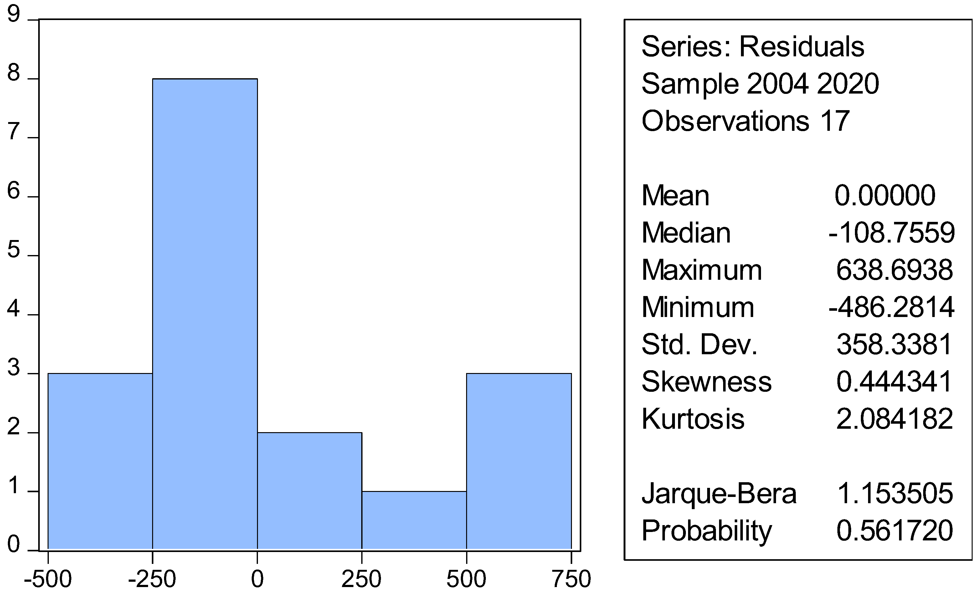
In addition, we tested the model for normality and heteroscedasticity using the Jarque Bera and ARCh tests, respectively, and found neither heteroscedasticity nor non-normality in the distribution of the residual (
Figure 1).
As can be seen from
Figure 1, the probability in the Jarque Bera test is above 0.05, proving that the residuals are normally distributed; in addition, the probabilities in the ARCH test (
Table 9) for heteroscedasticity (non-constant variance) are above 0.05, indicating the presence of homoscedasticity (constant variance). As the presumed conditions for building the ARDL model are met [
34], we can proceed with our analysis. In order to identify whether a long-term relationship between GDP per capita and inbound tourism exists, an F-Bounds Test was conducted (
Table 10).
From
Table 10, it is clear that the F-statistic is greater than the lower (I(0)) and upper (I(1)) bounds [
34]. Therefore, we can state that a long-term relationship between the explanatory and dependent variables exists. Below, the results of the ARDL (4,0) for the long-term relationship with real GDP per capita are shown in
Table 10.
According
Table 11, the long-term impact of real GDP per capita on the inbound tourism of Uzbekistan is significant at a 99% confidence level; however, it is much less than the short-term impact.
With regard to forecasting the number of inbound tourists in five years’ time, we used the ARIMA model. Here, we conventionally assigned Y to the number of inbound tourists. A stationary (constant mean and variance) time series is needed in order to use the ARIMA model to forecast values. In order to ensure this, we took the first difference of Y, namely,
. The result of the Augmented Dickey–Fuller test was significant at a 97% confidence level (
Table 12).
Also, for proper ARIMA model selection we inspected the dependent variable’s correlogram (
Table 13). It can be seen that in lag 2 the deviation is greatest, therefore it is better try building combination of ARIMA models with second lag.
Then, based on Box-Jenkins methodology, we checked ARIMA (2,1,2), ARIMA (2,1,0), and ARIMA (0,1,2). The ARIMA (2,1,2) and ARIMA (0,1,2) models turned out to be insignificant for either AR or MA processes. However, ARIMA (2,1,0) was significant at a 99% confidence level (
Table 14). According Box Jenkins methodology, we checked whether the residuals of ARIMA (2,1,0) were white noise (with zero mean and constant variance) using a correlogram. From
Table 15, it is clear that the
p-values for all lags are higher than 0.03, which means that all the lags are white noise with a 97% confidence level.
The graphical presentation of statistical data helps to quickly and easily identify unjustified peaks and troughs that clearly do not correspond to the displayed statistical data, anomalies, and deviations [
35].
The graphical presentation of statistical data is both a means of illustrating statistical data and of controlling their correctness and reliability [
36]. Due to its properties, it is an important means of interpreting and analyzing statistical data, and in certain cases is the only and indispensable way of generalizing and understanding them [
37]. In particular, it is indispensable for the simultaneous study of several interrelated economic phenomena, as it allows the relationships and connections existing between them to be established along with the difference and similarity while identifying the features of their changes over time.
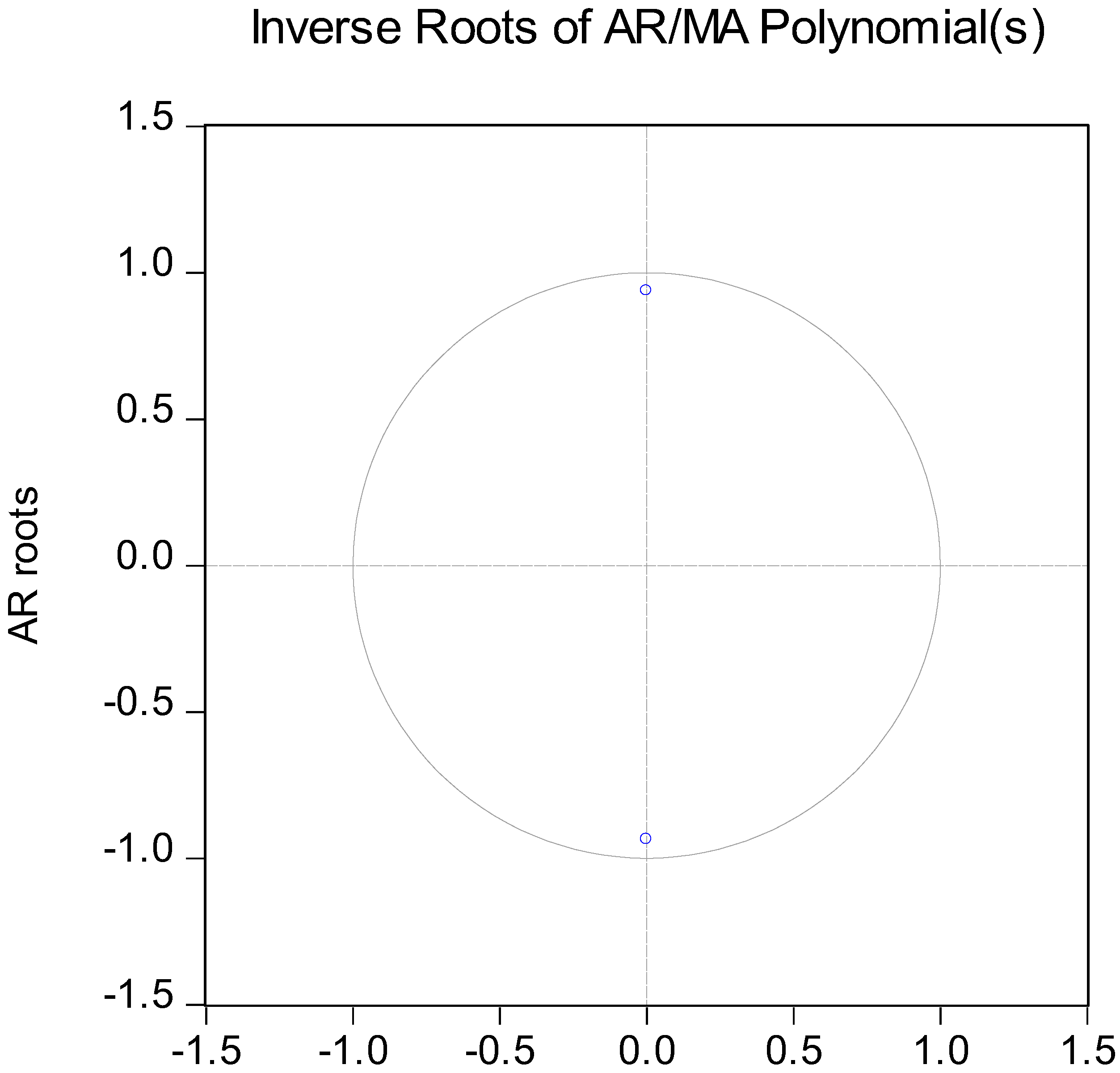
The next step was to verify whether the AR roots lie inside the unit circle; as can be seen in
Figure 2, the two AR roots indeed lie within the unit circle. Therefore, we are able to forecast the values using the ARIMA (2,1,0) model [
38].
Using Eviews 10, we forecasted the number of inbound tourists by applying the ARIMA (2,1,0) model. Algebraically, it can be formulated it in the following way:
Here,
α1, α2—corresponding coefficients,
σ—mean value, and
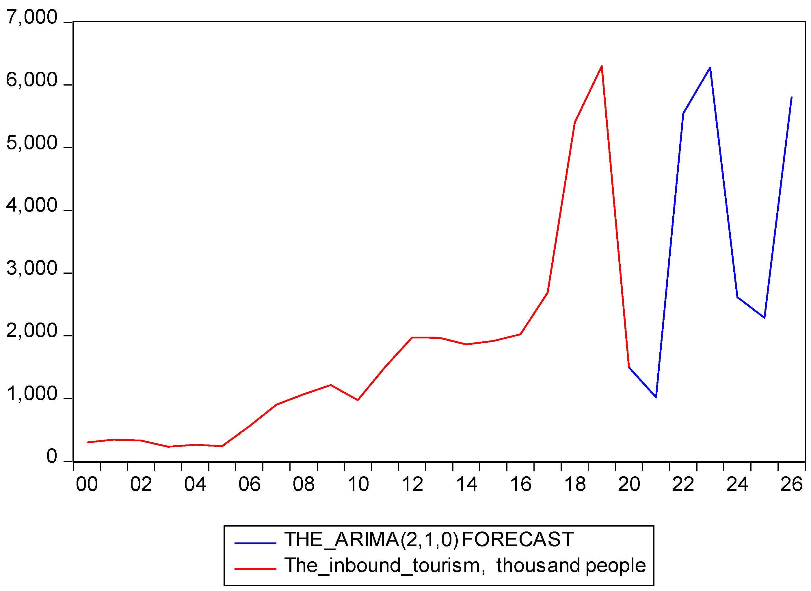
ut—uncorrelated random error term. The results of the forecasting are illustrated in
Figure 3.
The absolute forecast values for years from 2022 to 2026 are provided in
Table 16.
From
Table 11, it can be seen that the inbound tourism fell into a four-year cycle; however, the depth of cycle shortened as time passed. The forecast results can be interpreted as the number of tourists grows closer to pre-pandemic figures, after which there is a greater probability of a return of quarantine situation, when the number of inbound tourists may fall, after which demand slowly rises again. This process continues up to the point when public immunity against COVID-19 is reached.
5. Results
The results of multiple regression that aims to evaluate the impact of various factors on inbound tourism show the
model, that is, the impact of total recorded crimes, life expectancy, and consumer price index relative to the previous year. The R-squared for this model was 91%, the highest of all the competitive models. Based on the results from
Table 5, we can formulate the regression equation in the following way:
In other words, if total crimes recorded increases by 100, then the number of inbound tourists falls by five people, while if people’s life expectancy rate increment increases by one year then the number of inbound tourists increases by 1114 people. The life expectancy rate is an important indicator representing the level of development of a society. If the majority of people live in good conditions, then the probability of longer life increases, significantly boosting life expectancy rate. Thus, it is evident that better conditions for living attract more people from abroad.
The model
is important as well in terms of revealing the impact of passenger transportation volume. It can be written as follows:
That is, a rise in passenger transportation by one million people increases the number of inbound tourists by only one thousand people, if we consider a transportation network bearing more than a million passengers. The R squared is smaller than that of the first model, shaping 80%. The next
OLS model is important because it evaluates the impact of real GDP per capita on inbound tourism. Its equation can be written mathematically in the following way:
We can interpret the results of the regression in the following way. If the real GDP per capita grows by 100 thousand sums, the number of incoming tourists climbs by 27 people. The R-squared for this model accounted for only 68%, the lowest out of all three competitive models.
All three of the above-mentioned models can be used in practice to evaluate the indirect impact of welfare, crime, and the level of transportation network development on inbound tourism in Uzbekistan. This is important in strategic planning for the development of tourism infrastructure in various regions.
We decided to assess the lagged impact of the welfare (proxy real GDP per capita) on the inbound tourism using the ARDL model, which enables assessment of both short-term and long-term impacts of the explanatory variable on the dependent variable. For the short-term relationship we obtained the following results:
In other words, two- and four-year previous lags of inbound tourism negatively affect the contemporary inbound tourism, while an increase of 100 thousand sums in the real GDP per capita will increase the number of inbound tourists by 161 people.
The long-term relationship between real GDP per capita and inbound tourism can be formulated as follows:
As can be seen, the long-term effect of real GDP per capita is much less than the short-term effect. According to
Table 10, a one thousand-sum increase in real GDP per capita results in an increase of 285 people as inbound tourists. Remarkably, the long-term coefficient (0.285) from the ARDL (4,0) model is very close to the result obtained with the linear regression model (0.27), which indicates that the model is correctly specified.
With regard to the forecast of the number of incoming tourists, the ARIMA method was used. Having tested correlograms of various ARIMA models, we decided to use ARIMA (2,1,0) because only this model was significant for autoregressive processes, while in other variants, such as ARIMA (2,1,2) and ARIMA (0,1,2), either the MA or AR process was insignificant at the 95% confidence level. The results of the forecasting show that the shock of the COVID-19 pandemic will have a continuing effect until later then 2026. However, as time passes the fluctuations in the inflow of tourists smooth, eventually turning into an upward trend.
6. Discussion
In this study, we focused on evaluating the impact of certain factors representing welfare (GDP per capita, life expectancy, consumer price index), infrastructure (passenger transportation volume), the environment (CO2 emissions), and the security level (total crime records). However, out of these six factors, only four factors turned out to be statistically significant. CO2 emissions and consumer price index did not significantly affect inbound tourism. Other factors, for instance, life expectancy, GDP per capita, and passenger transportation volume, were strongly correlated with each other; therefore, each constituted a separate regression model. Out of three competitive models, the OLS model with the factors of life expectancy and total crime better explained the fluctuations in the inbound tourism.
The research results obtained by Biaggi [
20] demonstrated that a 1% increase in the number of tourists led to a 0.018% rise in total criminal activity in Italy. Moreover, the environmental impact of tourism can be detrimental, according to Sunlu [
21]. In his research, he points out loss of biodiversity, depletion of the ozone layer, climate change, and natural disasters as global threats to the environment are is partially caused by international tourism. As a way out, he proposes better tourism planning and management, in which statistical analysis is mostly used. Therefore, our research results can be helpful in this regard in planning sustainable tourism development.
We studied the lagged effect of real GDP per capita (consumption and welfare level) on inbound tourism using an ARDL model. According to our results, if welfare increases by one unit, the short-term effect on inbound tourism is eight times stronger than the long-term effect. It is evident from the dynamics of inbound tourism that from 2016, as the new government came into power, more and more funds were allocated for infrastructure between 2017 and 2021. Therefore, we can say that the results of our research correctly reflect the real dynamics of inbound tourism in Uzbekistan.
It was very difficult to assess the impact of the COVID-19 pandemic on international tourism considering the unprecedented and rapidly evolving crisis. The pandemic had a profoundly negative impact on the sustainable development of the tourism sector, as in all sectors of the economy. The number of foreign tourists visiting destinations around the world decreased by 74% in 2020 compared to 2019, while the loss from exports of tourist services reached USD 1.3 trillion, which is eleven times more than the loss due to the global financial and economic crisis in 2009 [
39].
In the worst-case scenario, this would result in a loss of USD 4 trillion in international tourism revenues (exports) in 2020–2021. These calculations, however, should be interpreted carefully, taking into account the scale, variability, and unprecedented nature of this crisis. The tourism sector is a major creator of jobs, especially for vulnerable groups such as women and youth.
Strict quarantine measures imposed due to the pandemic had a negative impact on tourism in Uzbekistan, as in all countries of the world. The reduction and complete abolition of the flow of foreign tourists visiting Uzbekistan has led to a sharp decline in exports of tourist services.
As a result, the number of tourists visiting Uzbekistan in 2020 decreased by 4.5 times compared to 2019 (6.3 million people), amounting to 1.5 million people. In turn, the volume of exports of tourist services decreased by 2.5 times (USD 1313.1 million in 2019) and amounted to USD 262.1 million. The decrease in the flow of tourists sharply reduced the activity of the network. In particular, in the first half of 2020, all tour packages were cancelled, while in the second half of the year almost half of all tour packages were cancelled.
7. Conclusions
Using the ordinary least squares model to evaluate the impact of factors reflecting welfare, infrastructure, security, and the environment, we show that the sense of welfare and security level strongly affect the volume of inbound tourism in the example of the Republic of Uzbekistan. Although we picked only factors that could partially cover the above categories, we did not intend to state that other factors had less effect on inbound tourism. Because of the complex nature of welfare, security, infrastructure, and the environment, we chose only their proxies. Further cross-country research is needed to examine the impact of welfare, security, the environment, and infrastructure development on inbound tourism. This may reveal more useful information about the constituents of tourism demand.
In order to verify whether the past (time lagged) values of any selected factor affect the dependent variable, we assessed various factors’ time lagged effects on inbound tourism. During a trial-and-error process using an autoregressive distributed lag model (ARDL), we ended up with a model of lagged real GDP per capita and past values of inbound tourism on the contemporary inbound tourism. One of the advantages of the ARDL model is that it enables researchers to evaluate the statistical relationship in both short- and long-term periods [
34]. The short-term effect of real GDP per capita appeared to exceed the long-term effect by eight times, which can be explained by the political changes that took place in 2016. Afterwards, the new government allocated more resources to the development of tourism infrastructure from year to year. With regard to the long-term effect, remarkably, it almost coincided with the results obtained by OLS regression, which can confirm the correct specification of our econometric model.
The indicators forecast here can be used in the development of tourism development strategy, and its implementation in a clear sequence can indicate which services will be in high demand in the future, in what volume, and how many times the number of potential customers can be expected to increase. In our study, we forecast the volume of inbound tourism using a time series-univariate ARIMA model. The results show that the impact of the COVID-19 pandemic will persist beyond then 2026. The shock of the pandemic was deep enough that it will not be easy to restore the pre-crisis level of tourism demand quickly.
The priority goal is to achieve aggregate growth of the tourism sector in 2022, primarily through the development of domestic tourism. In order to achieve the indicators of the pre-crisis period and ensure sustainable development, it is necessary to develop measures for both the medium- and long-term periods.
The post-crisis situation requires strategic planning in the tourism sector in order to ensure the sustainability of the sector through the implementation of long-term measures. During the COVID-19 pandemic, the government of Uzbekistan took measures to mitigate its negative impact through easing tax burdens and subsidizing local tourism companies. Now, the state is focused on supporting domestic tourism by encouraging people to travel within the republic. Efficient use of domestic resources can ensure the formation of a quality tourism product and allow the country to form an image of a destination with well-developed tourism infrastructure and rich tourism potential.
Throughout this, research we have evaluated the statistical impact of welfare, transport infrastructure, security, and the environment on the inbound tourism, or international tourism demand. Many well-known tourism specialists, such as L. Dwyer [
33], M. Porter [
40], P. Forsyth [
33], Ch. Kim [
41], B. Ritchie [
42], G. Crouch [
8,
42], and others have proposed models of competitive tourism destination. In these models they pointed out destinations’ environment, infrastructure, standard of living, and security level as key factors that shape competitiveness. Our research contributes to the “state of the art” as an empirical experiment on assessment of the impact of factors that form tourism competitiveness in terms of inbound tourism demand using the example of the Republic of Uzbekistan, which is considered an emerging destination. These research results can be used in strategic tourism planning in the different regions of Uzbekistan.


 ,
, 


