Study on the Spatial and Temporal Differentiation Pattern of Carbon Emission and Carbon Compensation in China’s Provincial Areas

Abstract

Excessive carbon emissions lead to global warming, which has attracted widespread attention in the global society. Carbon emissions and land use are closely related. An analysis of land use carbon emissions and carbon fairness can provide guidance for the formulation of energy conservation and emission reduction policies. This study uses data on agricultural production activities, land use and energy consumption and uses the carbon emission coefficient method to calculate carbon emissions and carbon absorption. The tendency value is used to analyze trends in land use carbon emissions and carbon absorption. The Gini coefficient, ecological support coefficient and economic contributive coefficient are used to analyze the fairness and difference of carbon emissions. The results showed that: (1) During the study period, there were fewer provinces with rapid growth in carbon emissions and carbon absorption and more provinces with slow growth. (2) Cultivated land and woodland are the main carriers of land use carbon absorption, and most provinces steadily maintain the type of carbon absorption to which they belong. (3) Carbon emissions from construction land are the main source of total carbon emissions, and the high concentration areas of carbon emissions are mainly located in the more economically developed areas. (4) There are obvious regional differences in the net carbon emissions. By 2015, Shanxi–Shandong High–High agglomeration areas and Yunnan–Guangxi Low–Low agglomeration areas were finally formed. (5) The distribution of carbon emissions in different provinces is not fair, and the spatial distribution is obviously different. Based on the analysis results, relevant suggestions are made from the perspectives of carbon emission reduction and carbon sink enhancement.

1. Introduction

China is in the process of rapid urbanization and industrialization, consuming a large amount of various fossil energy sources. At present, China’s carbon dioxide emissions have surpassed that of the United States, becoming the world’s largest carbon dioxide emitter [1]. With the rapid economic development and urbanization, the rapid population growth is accompanied by the large-scale use of various fossil energy sources [2]. Greenhouse gases continue to increase. Human activities emit large amounts of greenhouse gases, which contribute to the greenhouse effect and, ultimately, to global warming. The increase of carbon emissions will not only cause a series of problems, including global warming, but also endanger the sustainable development of human beings. In recent years, the warming of the climate system has become an indisputable fact. The issue of carbon emissions is also becoming more and more important for individual countries [3]. The fifth report of the IPCC of the United Nations Special Committee on Climate Change pointed out that, since industrialization, the increase in the carbon dioxide concentration has mainly been due to emissions caused by the burning of fossil fuels and changes in land use. From 1850 to 1998, the direct carbon emissions from land use and its changes accounted for one-third of the total carbon dioxide emissions from human activities, which had a very important impact on the global carbon cycle [4]. The impact of land use on carbon emissions has attracted widespread attention from various countries [5].

The carbon emission effect of land use has also been studied deeply and systematically by scholars in many countries [6]. Among them, some scholars have conducted in-depth research on the development of an agricultural soil carbon inventory in Ontario, Canada; the methods used to estimate carbon emissions range from simple empirical factors to complex process-based ecosystem models [7]. Critical gaps have been identified and improvements proposed that can be applied to developing countries in the future. Zuo et al. [8] deeply studied the land carbon emissions in Guangdong Province and found that the marginal carbon emission factor can reflect the real-time carbon emissions of the system more accurately. The results showed a significant increase in the marginal carbon emission factor for the peak demand time. Some researchers have studied the relationship between urban sprawl and carbon emissions in the metropolitan area of Monterrey, Mexico [9]. Lai et al. conducted research on carbon emission assessment and carbon reduction strategies in newly urbanized areas, selecting three different new urban areas for analysis; relevant emission reduction strategies were planned and implemented [10].

In terms of model methods and data, Lv et al. [11] used the panel data of 11 cities in Jiangxi Province from 2007 to 2018, and Driscoll–Kraay estimation was used to explore the impact and effect of econometrics on emissions. Studies have shown that population, economy, energy and social urbanization play positive roles in promoting carbon emissions, while ecological urbanization plays a positive role in blocking carbon emissions. Luo et al. [12] used the AIM/ENDUSE model to analyze the changes and differences of the Great Bay Area (GBA) installed capacity, power supply, energy consumption and carbon emissions under different auction ratios and price combinations. The research also explores the best way to carry out energy transformation in the power industry of GBA. Using Landsat measurements to measure carbon emissions, which are also common, Chinese scholars have calculated the number of urban agglomerations in the Yangtze River Delta. Additionally, in the past 20 years, urban land carbon emissions increased about twice as much as urban land area [13]. The quantification of the CO₂ released by gases into the atmosphere is relevant for the evaluation of the balance between deep derivation, biogenic and anthropogenic contributions [14]. Zhang et al. [15] conducted in-depth research on the Yellow River Basin of China. They analyzed the spatial and temporal distribution characteristics of carbon emissions in the Yellow River from 2000 to 2019 by constructing a carbon emission model, carbon footprint and Moran’s I index. Due to the size of China’s population, the impact of China’s population aging problem on household carbon emissions is also significant, Fan et al. [16] found that rural population aging has a significant positive effect on household carbon emissions in northern heating regions. Through the analysis of its potential mechanism, it is determined that the consumption structure and consumption level are the mediating factors that influence the nonlinear relationship between urban population aging and urban household carbon emissions.

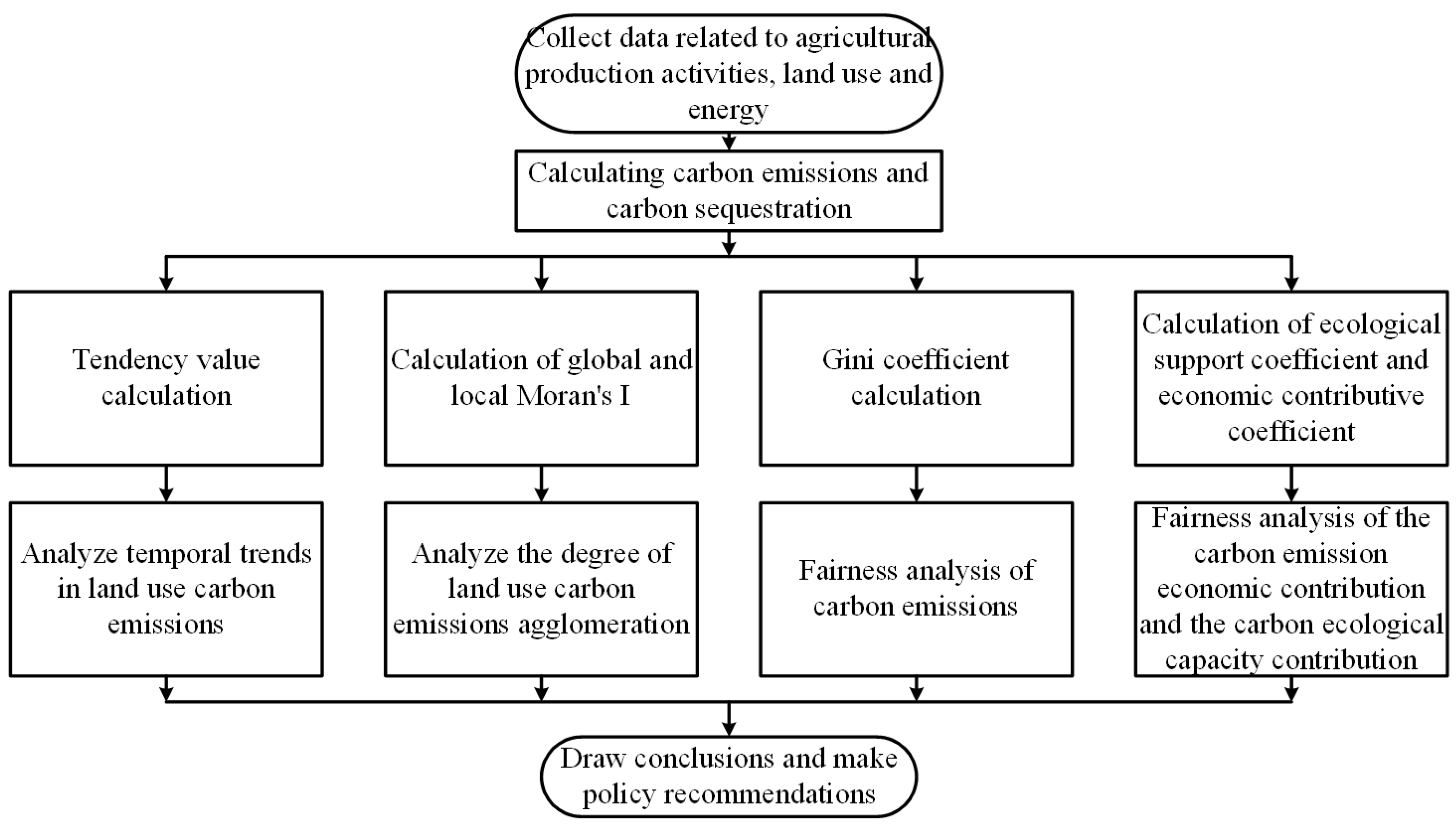
This paper takes 30 provincial administrative units in China as the study area to explore the spatial and temporal evolution of land use carbon emissions, carbon absorption and net carbon emissions in China’s provinces from 2003 to 2016 and analyzes the fairness and variability of carbon emissions through the Gini coefficient, ecological support coefficient and economic contributive coefficient of land use carbon emissions based on a spatial and temporal analysis. A relevant study on land use carbon compensation was also conducted. This paper analyzes the pattern of land use carbon sources and carbon absorption in China as a whole and provides a reference basis for advocating energy conservation and emission reduction and developing a regional low-carbon economy in China. This paper is important for improving the efficiency of carbon emission reduction task allocation in each province and further understanding the intrinsic mechanism of land use carbon emissions.

2. Materials and Methods

2.1. Data Sources

The data used in this study mainly includes: land use, GDP, population, energy consumption and agricultural production activities from 30 provincial administrative regions of China (excluding the Tibet Autonomous Region, Hong Kong Special Administrative Region, Macao Special Administrative Region and Taiwan Province). The land use data mainly came from the land survey results from the: “China Statistical Yearbook”, “China Land and Resources Statistical Yearbook”, “China Environmental Statistical Yearbook” and the National Land Use Planning Outline (2006–2020); energy consumption comes from the “China Energy Statistical Yearbook”; agricultural production activities data are from the “China Rural Statistical Yearbook”, “China Agricultural Statistical Data” and “Compilation of Agricultural Statistical Data for 30 Years of Reform and Opening up” and the data of the population and GDP are from the “China Statistical Yearbook”. The land use types in the IPCC Good Practice Guide on Land Use, Land Use Change and Forestry include woodland, grassland, farmland, wetland, residential area and other land. The data used in this study mainly come from the China Statistical Yearbook. The data on factors such as climate and soil are not recorded in the China Statistical Yearbook. This article does not consider soil, climate, hydrology and topography. These statistical data are used to calculate various indicators, such as land use carbon absorption, carbon emissions, ecological support coefficient and economic contributive coefficient. Remote sensing imagery data were obtained from the Resource and Environmental Science Data Center of the Chinese Academy of Sciences (http://www.resdc.cn, accessed on 1 April 2022).

2.2. Research Methods

This paper uses a variety of calculation methods to conduct research, and the research on carbon absorption is mainly for woodland, grassland and cultivated land [17]. The research on carbon emissions is mainly for cultivated land and construction land. Through the two spatial pattern analysis methods of spatial autocorrelation and local autocorrelation, not only the degree of agglomeration of similar spatial attributes can be known, but the spatial location of the agglomeration area can also be pointed out. The two methods are complementary to each other. The calculation of the ecological support coefficient (ESC) can reflect the carbon sink capacity of the area, and the relative level of the carbon ecological capacity can be judged by determining the relationship between the ESC and 1. We also calculated the SLOPE value to reflect the rate of increase in the carbon emissions. In the following, we will describe how we calculate the SLOPE and ESC. The economic contributive coefficient is used to measure the fairness of the regional carbon emission contributions from an economic point of view. The calculation of the value of the land use carbon compensation can be used as the benchmark value of land use carbon compensation, and it is an important measure of the area’s access to compensation funds. It can effectively understand and analyze China’s provincial carbon emissions in terms of time and space and contain deeper research on the regional distribution of carbon compensation. Figure 1 shows the research framework of this paper.

2.2.1. Carbon Emission Coefficient Method

This study investigates the effect of land use carbon emissions at the national scale, focusing on four major land use types: woodland, grassland, cultivated land and construction land. Figure 2 shows the land use of China from 2005 to 2015. Carbon absorption is mainly calculated for land use types such as woodland, grassland and cropland. Land use carbon emissions mainly include two types of carbon emissions from construction land and cropland [18]. Among them, cropland is both a carbon source and a carbon sink [19].

(1)

Carbon absorption in woodland and grassland

The calculation methods of carbon absorption in forest and grassland are as follows [20]:

$$C_i=S_i\times {\beta }_i$$

(1)

C_i is the carbon absorption of land type i, S_i is the area of land type i and β_i is the carbon absorption coefficient of land type i. The carbon absorption coefficients of woodland and grassland are 3.81 t/hm² and 0.91 t/hm² [21]. hm denotes hectares.

(2)

Carbon absorption of cultivated land

$$C{I}_{crop}={\displaystyle \sum _{i}C{I}_{crop-i}}={\displaystyle \sum _i{C}_{crop-i}}\times (1-P_{water-i})\times \frac{Y_{eco-i}}{H_{crop-i}}$$

(2)

CI_crop is the photosynthetic carbon absorption of crop i during the reproductive period. CI_crop-i is the carbon absorption of crop i. C_crop-i is the carbon absorption rate per unit of organic matter (dry weight) synthesized by the photosynthesis of crop i. P_water-i is the water content of crop i. Y_eco-i is the economic yield of crop i. H_crop-i is the economic coefficient of crop i. In this paper, we mainly calculate the carbon absorption of rice, wheat, maize, beans, potatoes, hemp, sugar beet, roasted tobacco, sorghum and grain crops. The crop economic coefficients, carbon absorption rates and average water content are from previous studies [22].

(3)

Carbon emission from cultivated land

Farmland is a carbon source because of the crop cultivation methods and includes the carbon emissions caused by the use of chemical fertilizers, agricultural irrigation, agricultural machinery, pesticides and agricultural film consumption [23]. The formula is as follows:

$$E_t=G_{f}A+T_{p}B+(S_{m}C+P_{m}D)+F_{a}E+A_{i}F$$

(3)

E_t are carbon emissions from cropland; G_f, T_p, P_m, S_m, F_a and A_i are fertilizer use, pesticide use, crop planting area, total agricultural machinery power, irrigated area and agricultural film use. A, B, C, D, E and F are the conversion factors, A and B values are from Oak Ridge Laboratory, USA: 0.8956 kg/kg and 4.9341 kg/kg, respectively. C, D and E were 16.47 kg/hm², 0.18 kg/kW and 266.48 kg/hm² [24]. F was 5.18 kg/hm² from the Institute of Agricultural Resources and Ecological Environment (IREEA), Nanjing Agricultural University.

(4)

Carbon emission from construction land

The human production and living activities carried out by the construction land consume a large amount of energy, and the calculation of its carbon emission is done by indirect estimation [25], which means that the energy consumption of coal, oil and natural gas in the production and living process is converted into standard coal, and then, the carbon emission of the construction land is calculated according to the carbon emission coefficient of each type of energy. In this paper, eight main energy sources: namely, raw coal, coke, crude oil, fuel oil, gasoline, kerosene, diesel and natural gas, are selected for calculation according to the actual situation, and the formula is as follows.

$$E_p={\displaystyle \sum e_i}={\displaystyle \sum E_i}\times {\theta }_i\times {\beta }_i$$

(4)

E_p is the carbon emission from construction land, e_i is the carbon emission from various fossil energy sources, E_i is the consumption of various fossil energy sources, θ_i is the coefficient of conversion of various fossil energy sources into standard coal in the appendix of the China Energy Statistical Yearbook and β_i is the carbon emission coefficient of various fossil energy sources in the IPCC Guidelines for National Greenhouse Gas Emission Inventories.

2.2.2. Tendency Value Calculation

Linear propensity estimation enables the analysis of temporal trends in land use carbon emissions. A one-dimensional linear regression model of land use versus time was developed. The SLOPE of temporal change from 2003 to 2016 was calculated to analyze the linear tendency of land use CO₂ emissions for each city [26].

$$\mathrm{SLOPE}=\frac{n\times {\displaystyle \sum _{i=1}^n{X}_i{C}_i-{\displaystyle \sum _{i=1}^n{X}_i{\displaystyle \sum _{i=1}^n{C}_i}}}}{n\times {\displaystyle \sum _{i=1}^n{X}_i^2-{\left({\displaystyle \sum _{i=1}^n{X}_i}\right)}^2}}$$

(5)

In this formula: n is the total number of years, equal to 14; X_i is the year i (2003 is the first year) and C_i represents energy CO₂ emissions for year i. When SLOPE > 0, increased over time t, carbon emissions are on the rise. When SLOPE < 0, increased over time t, carbon emissions are on a downward trend. The SLOPE value reflects the rate of increase or decrease in carbon emissions and indicates the degree of tendency to increase or decrease. When the tendency value was calculated, we classified the change trends into five categories: slow growth, slower growth, medium growth, faster growth and rapid growth. The change types were classified according to the tendency value using the natural breakpoint method.

2.2.3. Spatial Pattern Analysis Method

Spatial autocorrelation analyzes the correlation of the same variable in different spatial locations and is a measure of the degree of agglomeration in the space domain [27]. Depending on the size of the spatial range analyzed, space self-correlation can be divided into global spatial autocorrelation and local spatial autocorrelation [28].

The most commonly used global spatial self-correlation is Moran’s proposal Global Moran′s I [29]. The calculation formula for Global Moran′s I is as follows:

$$I=\frac{{\displaystyle \sum _{i=1}^n\left(X_i-\overline{X}\right){\displaystyle \sum _{j=1}^n{W}_{ij}}\left(X_j-\overline{X}\right)}}{S^2{\displaystyle \sum _{i=1}^n{\displaystyle \sum _{j=1}^n{W}_{ij}}}}$$

(6)

$$s^2=\frac{1}{n}{{\displaystyle \sum _{i=1}^n\left(X_i-\overline{X}\right)}}^2$$

(7)

where n is the number of space units, X_i; X_j represents the sites on the property values of space units i and j and W_ij is the spatial weight coefficient matrix and represents the proximity of each space unit.

Global Moran′s I is a comprehensive measurement of spatial autocorrelation self-related to the research area. Although it can see the degree of aggregation of similar properties of space, it cannot accurately indicate the spatial position of the aggregation area. Global Moran′s I can make up for this defect very well. Local Moran’s I can be obtained by Formulas (8) and (9):

$$I=\frac{\left(X_i-\overline{X}\right)}{s^2}{\displaystyle \sum _{j=1}^n{W}_{ij}}\left(X_j-\overline{X}\right)$$

(8)

$$I_i=\frac{n\left(X_i-\overline{X}\right){\displaystyle \sum _{j=1}^n{W}_{ij}}\left(X_j-\overline{X}\right)}{{\displaystyle \sum _i{\left(X_i-\overline{X}\right)}^2}}=Z_i{}^{\text{'}}{\displaystyle \sum _i{W}_{ij}{Z}_j{}^{\text{'}}}$$

(9)

In this formula: X_i and X_j represent the property values of the space units i and j, W_ij is a spatial weight coefficient matrix that represents the proximity of each space unit and Z_i′ and Z_j′ are standardized observations by standard deviation.

When I_i > 0, the regional space unit i has a strong positive spatial self-correlation with the observation properties of adjacent space units, local spatial aggregation; when I_i < 0, there is a strong negative spatial self-correlation, which is a partial spatial dispersion.

2.2.4. Calculation of the GINI Coefficient of Carbon Emissions from Land Use

In this paper, 30 provincial-level administrative regions are used as evaluation units, and the Lorenz curve (Figure 3) is defined as the land use carbon emission curve of different units [30]; that is, the actual distribution curve of land use carbon emissions, and the 45 degree diagonal line is the absolute fairness curve of the land use carbon emissions [31]. The area between the absolute fair curve of land use carbon emissions and the actual distribution curve is A, and the area between the actual distribution curve of land use and the X-axis is B; the Gini coefficient = A/(A + B). When the Gini coefficient is larger, it means the greater the inequality in income distribution. A Gini coefficient below 0.2 is for a high average gap, 0.2 to 0.3 for a relative average gap, 0.3 to 0.4 for a typical gap, 0.4 to 0.5 for a large gap and 0.5 or more for a very large gap. The Gini coefficient equal to 0.4 is usually considered as a “red line” for carbon equity.

Using the trapezoidal method to calculate the Gini coefficient of carbon emissions, the formula is as follows [32]:

$$Gini coefficien=1-{\displaystyle \sum _{i=1}^n(X_i}-X_{i-1})(Y_i+Y_{i-1})$$

(10)

X_i is the cumulative percentage of carbon absorption, and Y_i is the cumulative emission ratio of carbon emissions; when i = 1, both X_i−1 and Y_i−1 are 0.

2.2.5. The Calculation of Ecological Support Coefficient and Economic Contributive Coefficient

The ecological support coefficient is an indicator to measure the equity of the contribution of the carbon ecological capacity in each province and reflects the region’s carbon sink capacity [33]. CA_i and CA are the carbon absorption of each province and the country; C_i and C are the provinces and the national carbon emissions.

$$ESC=\frac{C{A}_i}{CA}/\frac{C_i}{C}$$

(11)

If ESC > 1, the contribution rate of carbon absorption in one province is greater than the contribution rate of carbon emissions, which indicates that it has a relatively high carbon ecological capacity and contributes to other provinces. Conversely, if ESC < 1, the carbon ecological capacity is relatively low.

The economic contributive coefficient is an economic measurement of the equity of the contribution of carbon emissions between regions, reflecting in the region’s carbon productivity [33]. G_i and G are the provinces and the national GDP; C_i and C are the provinces and the national carbon emissions of land use.

$$ECC=\frac{G_i}{G}/\frac{C_i}{C}$$

(12)

If ECC > 1, this indicates that the contribution rate of a province′s economy is greater than that of carbon emissions, which shows that it has a high economic efficiency and energy utilization efficiency, and the carbon productivity is strong. Conversely, if ECC < 1, this indicates that its carbon productivity is weak.

3. Results and Discussion

3.1. Trends in Carbon Emissions and Carbon Absorption Time in Provinces

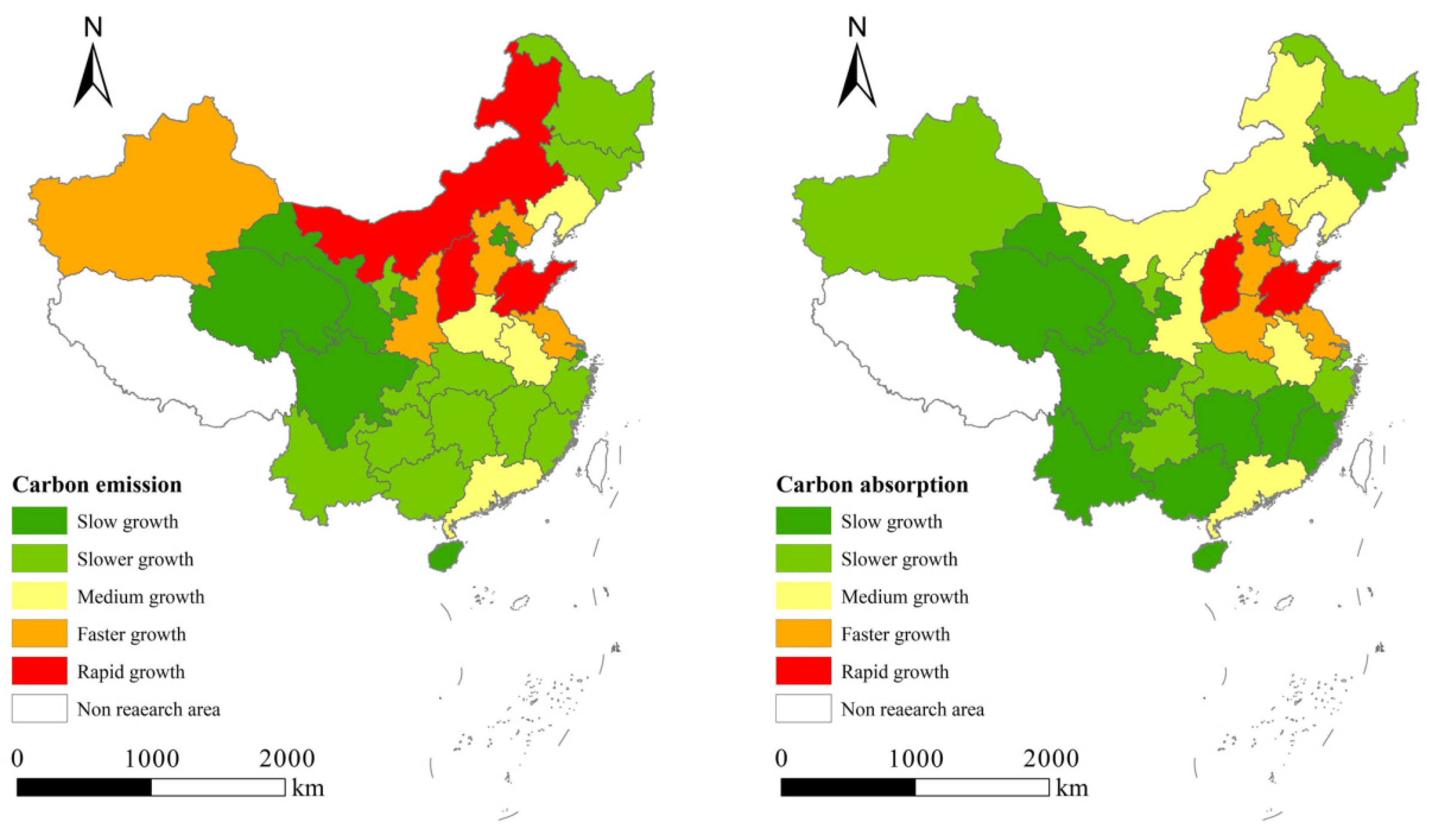
To further clarify the temporal trends of land use carbon emissions and carbon absorption in each province, this paper calculated the tendency values of the total land use CO₂ emissions and absorption in each province of China from 2003 to 2016 using a trend analysis. The natural breakpoint method of ArcGIS was used to divide the growth trend of CO₂ emissions and total absorption of land use in each province into five types: slow growth, slower growth, medium growth, faster growth and rapid growth.

The carbon emission results show (

Table 1. Types of growth trends in the total CO₂ emissions by provinces.

Class	SLOPE Range	Province	Total
Slow growth	0.20–0.41	Qinghai, Gansu, Hainan, Beijing, Chongqing, Shanghai, Tianjin	7
Slower growth	0.41–0.63	Sichuan, Yunnan, Guizhou, Guangxi, Hunan, Hubei, Jiangxi, Fujian, Zhejiang, Jilin, Heilongjiang, Ningxia	12
Medium growth	0.63–1.57	Liaoning, Henan, Anhui, Guangdong	4
Faster growth	2.57–2.8	Xinjiang, Shanxi, Hebei, Jiangsu	4
Rapid growth	2.8–5.6	Inner Mongolia, Shanxi, Shandong	3

) that three provinces in China are of the rapid growth type and four provinces are of the faster growth type, concentrated in the west, as well as the middle reaches of the Yellow River (Figure 4), mainly due to the rapid growth of arable land and construction land area in these areas. Seven provinces in China belong to the slow growth type, and 12 provinces belong to the slower growth type concentrated in the northwest, southwest and southern coastal areas, as well as the northeast, mainly due to the relatively low level of economic development in these provinces and the land use is mostly woodland and grassland. With the continuous expansion of the woodland and grassland areas, carbon emissions grow slowly.

The results of the carbon absorption (

Table 2. Types of growth trends in the total CO₂ absorption by provinces.

Class	SLOPE Range	Province	Total
Slow growth	0.11–0.21	Qinghai, Gansu, Sichuan, Yunan, Guangxi, Hunan, Jiangxi, Fujian, Jilin, Hainan, Beijing	11
Slower growth	0.21–0.71	Guizhou, Heilongjiang, Ningxia, Xinjiang, Chongqing, Guizhou, Hubei, Zhejiang, Tianjin	9
Medium growth	0.71–1.27	Liaoning, Shanxi, Anhui, Guangdong, Inner mongoria	5
Faster growth	1.27–2.12	Henan, Hebei, Jiangsu	3
Rapid growth	2.12–3.11	Shanxi, Shandong	2

) show that two provinces in China are of the rapid growth type and three provinces are of the faster growth type, concentrated in the middle reaches of the Yellow River and the northern coastal areas (Figure 4). Due to the development of agricultural production, scientific and technological progress, the crop yield per unit area significantly increased; therefore, the carbon sequestration capacity of the crops during the reproductive period also increased, and the rate of the carbon absorption grew rapidly. Eleven provinces in the country are designated as slow growth, and nine provinces are slower growth and are concentrated in the northwestern, southwestern, southern coastal areas and northeastern regions. This is mainly because of the development of the western development strategy back to forest, pasture and grass. However, because of the slow increase in woodland and grassland areas, the growth of CO₂ absorption is slow.

3.2. The Characteristics of Space–Time Distribution of Carbon Absorption in Land Use

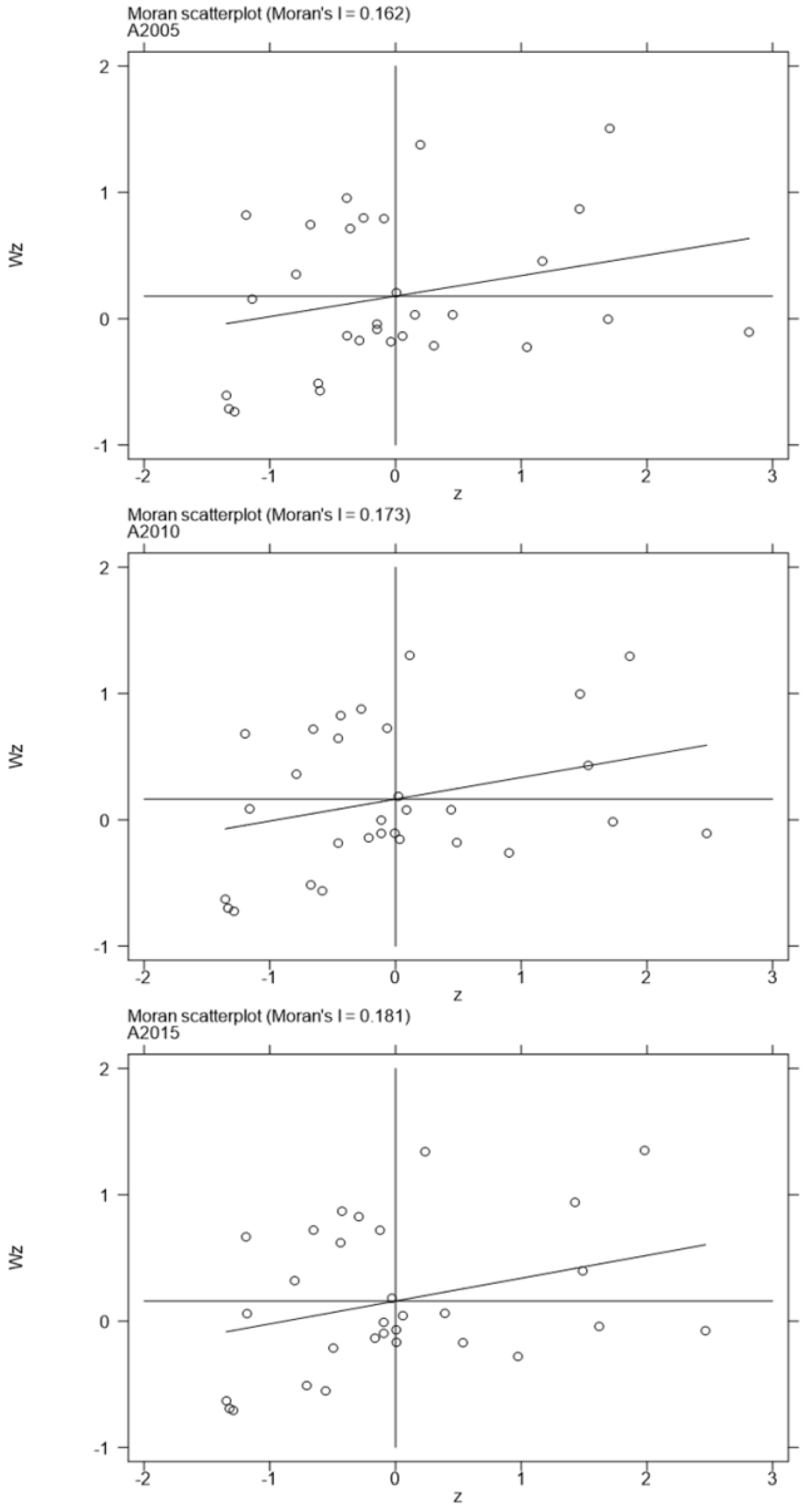
The global Moran’s I index reflects the aggregate change of the national land use CO₂ absorption distribution. The global Moran’s I indices for 2005, 2010 and 2015 were 0.162, 0.173 and 0.181. The index is positive at the 1% significance level and shows an upward trend. Scatter plots, as shown in Figure 5, show that there was a spatial positive correlation in CO₂ absorption, and the correlation gradually increased during the study period.

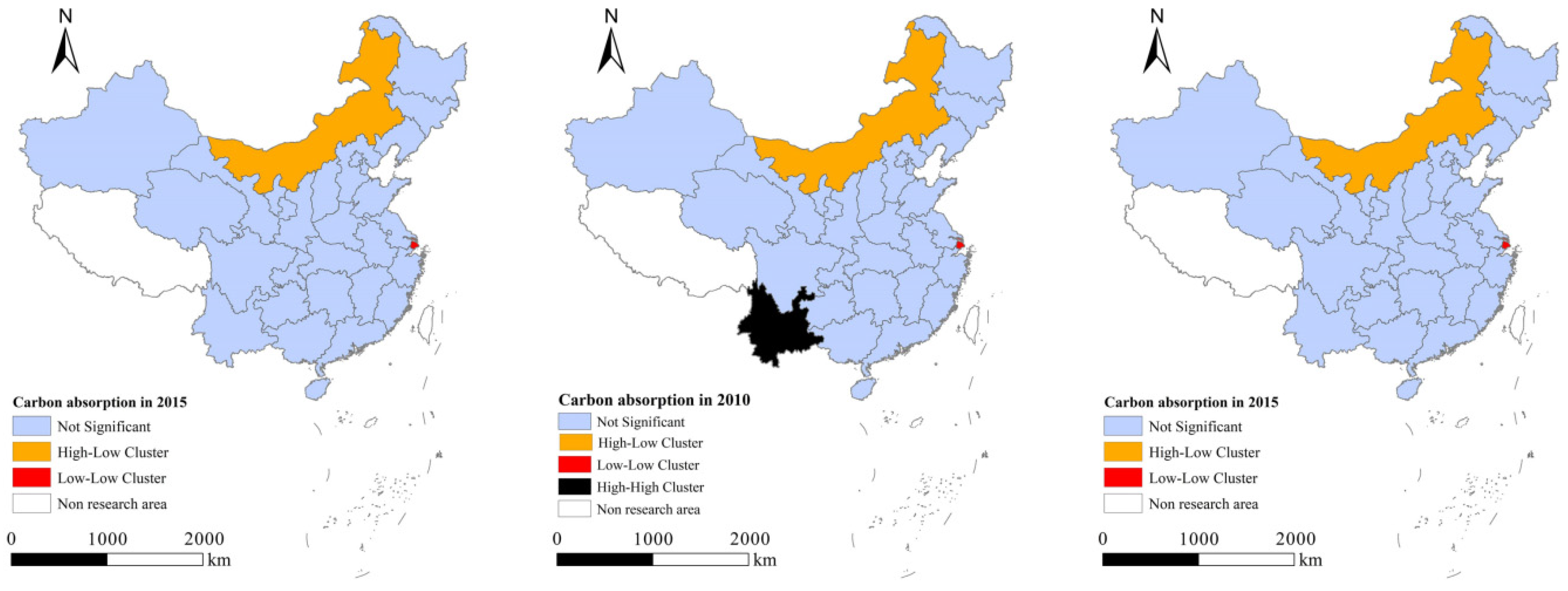
In order to analyze the spatial aggregation type of CO₂ absorption in land use, the LISA index of 30 provinces was calculated, and four types of High–High Cluster, High–Low Outlier, Low–High Outlier and Low–Low Cluster were calculated according to the LISA index.

The results found a High–Low Outlier area in Inner Mongolia, a Low–Low Cluster has formed in Shanghai and a High–High Cluster was formed in Yunnan in 2010 (Figure 6). The Inner Mongolian grassland area is large and is seen as the main carrier of carbon absorption. The area of cultivated land and woodland in Shanghai is small, and the carbon absorption is relatively small. In 2010, the State Council approved an overall land use plan for Yunnan Province, with special emphasis on strengthening the protection of cultivated land, especially basic farmland, strictly controlling the occupation of cultivated land by non-farm construction, increasing the intensity of supplementary cultivated land and strengthening the protection and construction of basic farmland, stabilizing the quantity and improving the quality so the CO₂ absorption is higher.

3.3. Space-Time Distribution Characteristics of Carbon Emissions from Land Use

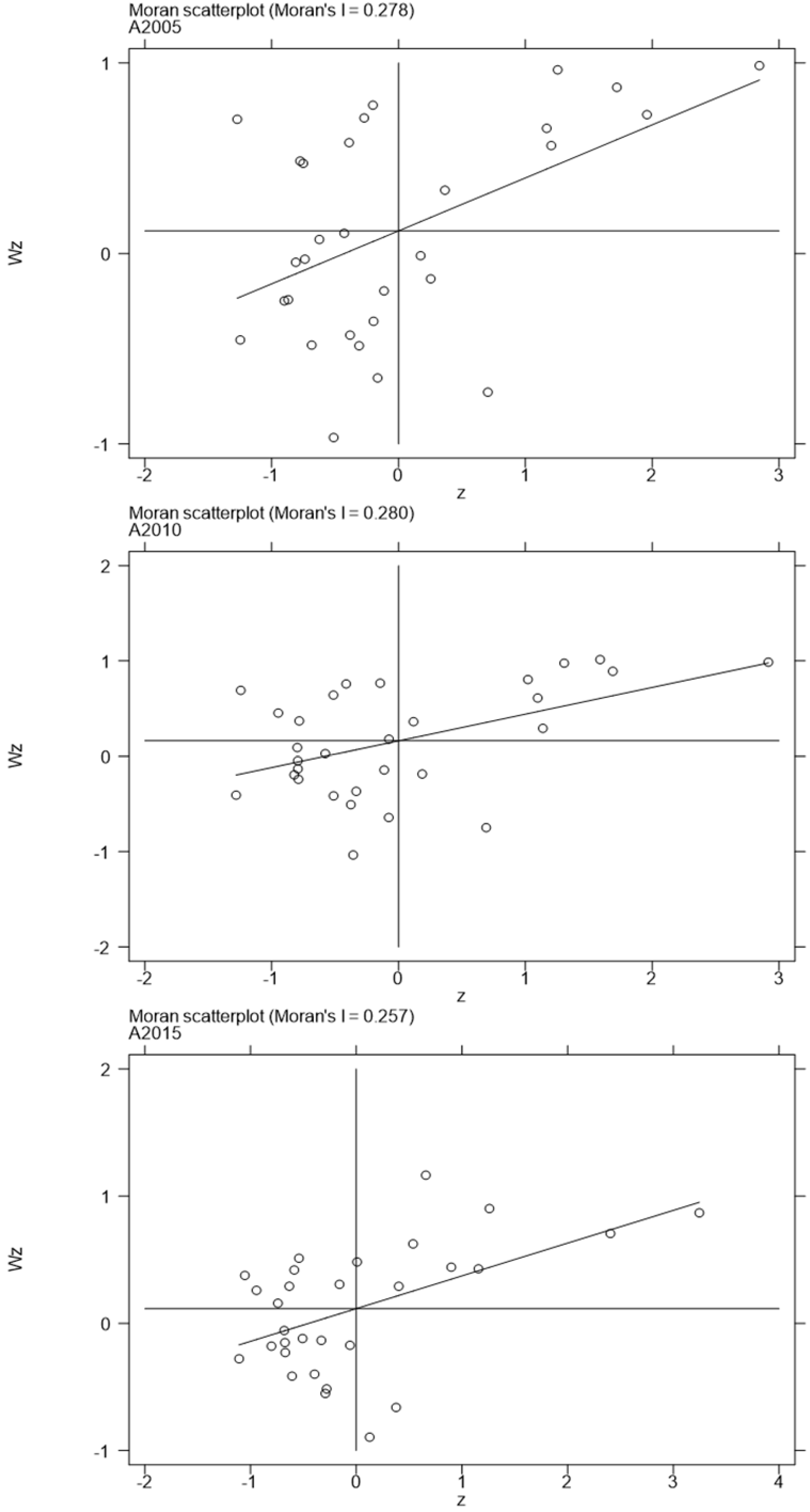
As shown in Figure 7, the global Moran’s I indices of the 30 provinces in 2005, 2010 and 2015 were 0.278, 0.280 and 0.257, showing significant spatial clustering. The significance showed a trend of increasing first and then decreasing. It can be seen that carbon emissions show a positive spatial autocorrelation on the whole, and the clustering in the sub-quadrants is more prominent. This shows that China’s provincial carbon emissions mainly show High–High and Low–Low spatial agglomeration characteristics, indicating that China’s provincial carbon has a high spatial dependence.

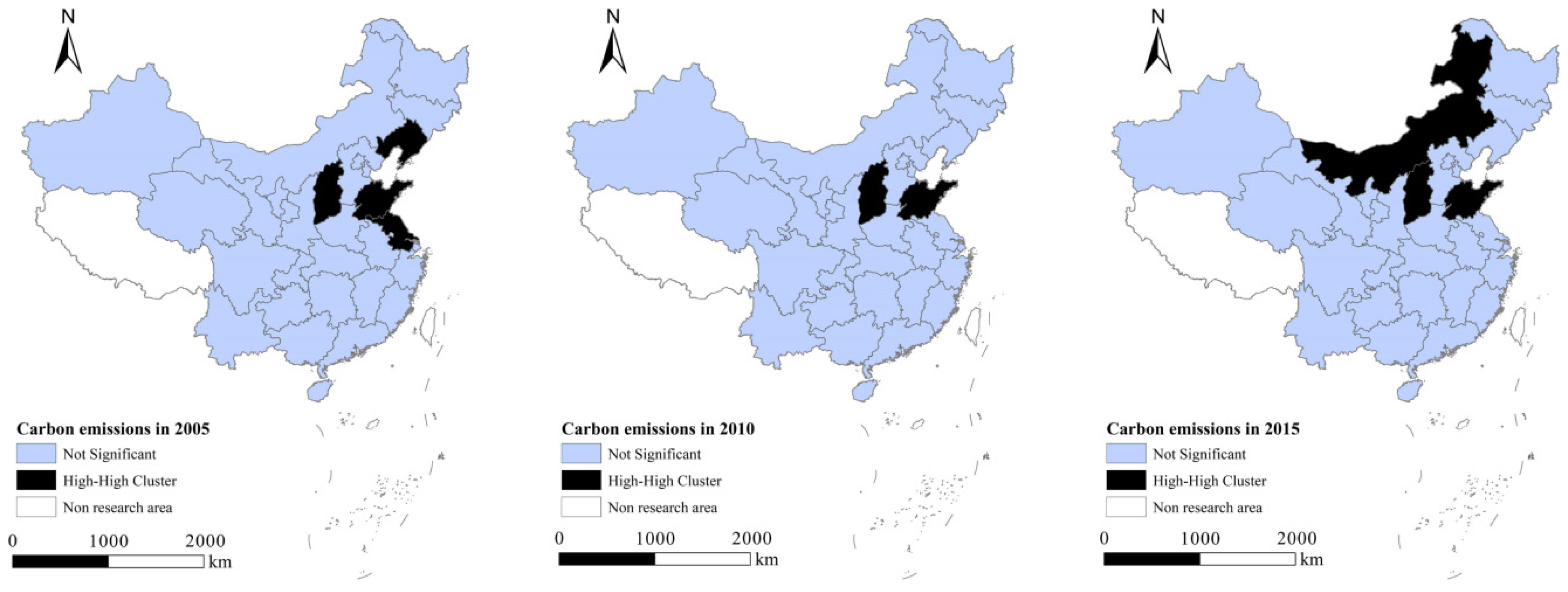
It was found (Figure 8) that high-value carbon emission communities were formed in Liaoning, Shanxi, Shandong and Jiangsu. The high-value carbon emissions in 2015 were concentrated in Shanxi, Shandong and Inner Mongolia. Shanxi Province is a famous coal-producing area in the country, and its energy structure is dominated by coal. Shanxi Province is a typical coal-based energy economy. Rapid economic development has accelerated the massive increase in carbon emissions. Shandong Province has experienced rapid economic development in recent years, urbanization and industrialization have progressed rapidly and much cultivated land has been converted into construction land. The increase in construction land is an important reason for the high concentration of carbon emissions in Shandong Province. In 2005, the carbon emissions of Inner Mongolia showed a high concentration, which was due to the fact that there are many industries with high energy consumption in Inner Mongolia, and the construction land area of Inner Mongolia is gradually expanding.

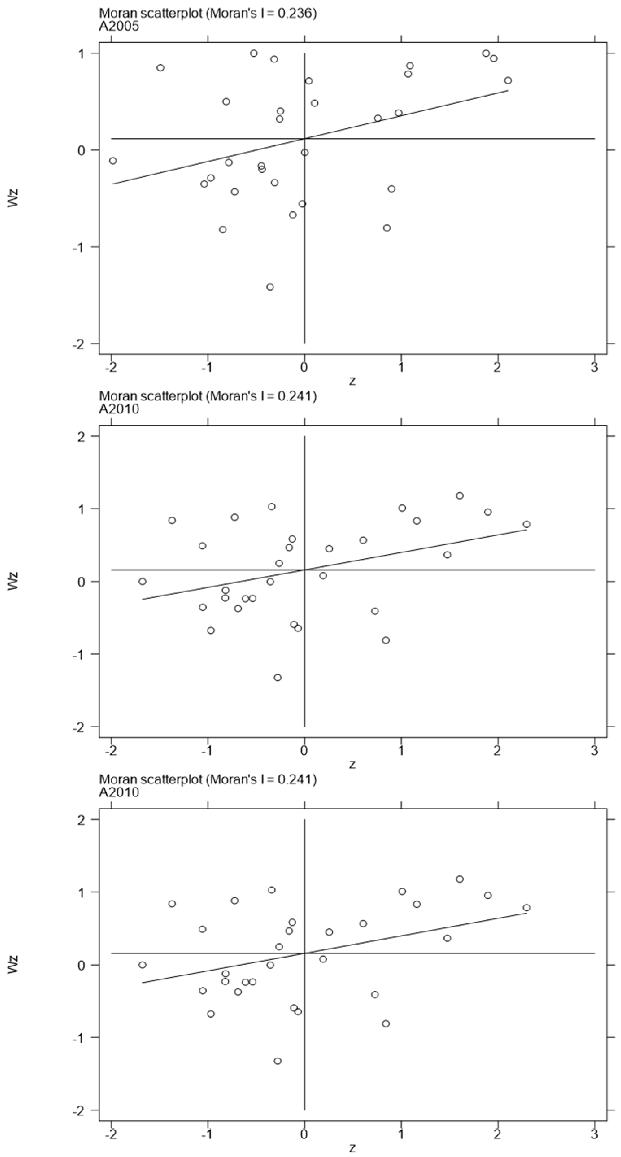
3.4. Spatiotemporal Distribution of Net Carbon Emissions from Land Use

As shown in Figure 9, the global Moran’s I of the 30 provinces in 2005, 2010 and 2015 were 0.236, 0.241 and 0.241, showing significant spatial clustering. It can be seen from Figure 9 that the total net carbon emissions show a positive spatial autocorrelation on the whole, and the clustering in the sub-quadrants is more prominent. The provinces are mainly concentrated in the first and third quadrants, and there are fewer provinces in the fourth quadrant. This shows that the total net carbon emissions in China’s provinces mainly show High–High and Low–Low agglomeration. When the Low–High situation appeared in 2005, it indicated that there was a spatial connection form in which the low net carbon emission area was surrounded by the high net carbon emission area, and there was a strong negative spatial correlation and significant heterogeneity.

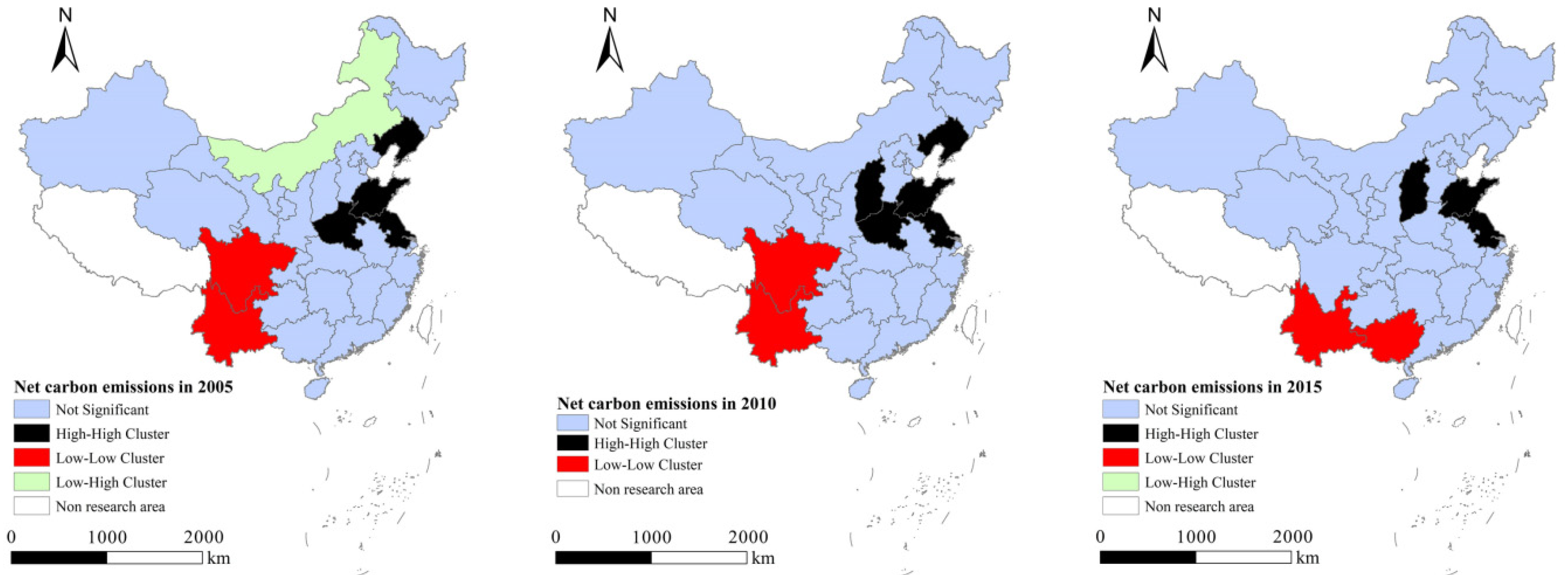
It was found (Figure 10) that a Low-High Outlier was formed in Inner Mongolia in 2005. It can be seen that Inner Mongolia is affected by the surrounding high agglomeration areas, such as Liaoning and Shanxi. The High-High cluster of net carbon emissions was mainly in Shanxi, Henan, Shandong and Liaoning. This is due to the large area of construction land in these provinces, the rapid economic development in recent years and the large energy consumption. By 2015, Liaoning and Henan were no longer high-value clusters. This is because Liaoning and Henan Provinces have adjusted their energy-intensive industries in response to the national emission reduction policy. In 2005, a Low-Low cluster was formed in Sichuan and Yunnan. By 2015, the Yunnan-Guangxi Low-Low Cluster was finally formed. This is because the two provinces of China, Yunnan and Guangxi, have vast forest areas and a strong carbon absorption capacity.

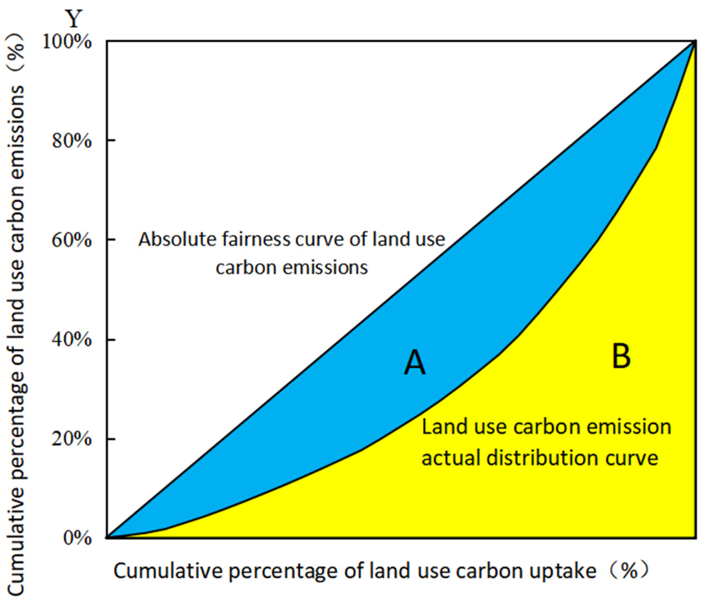
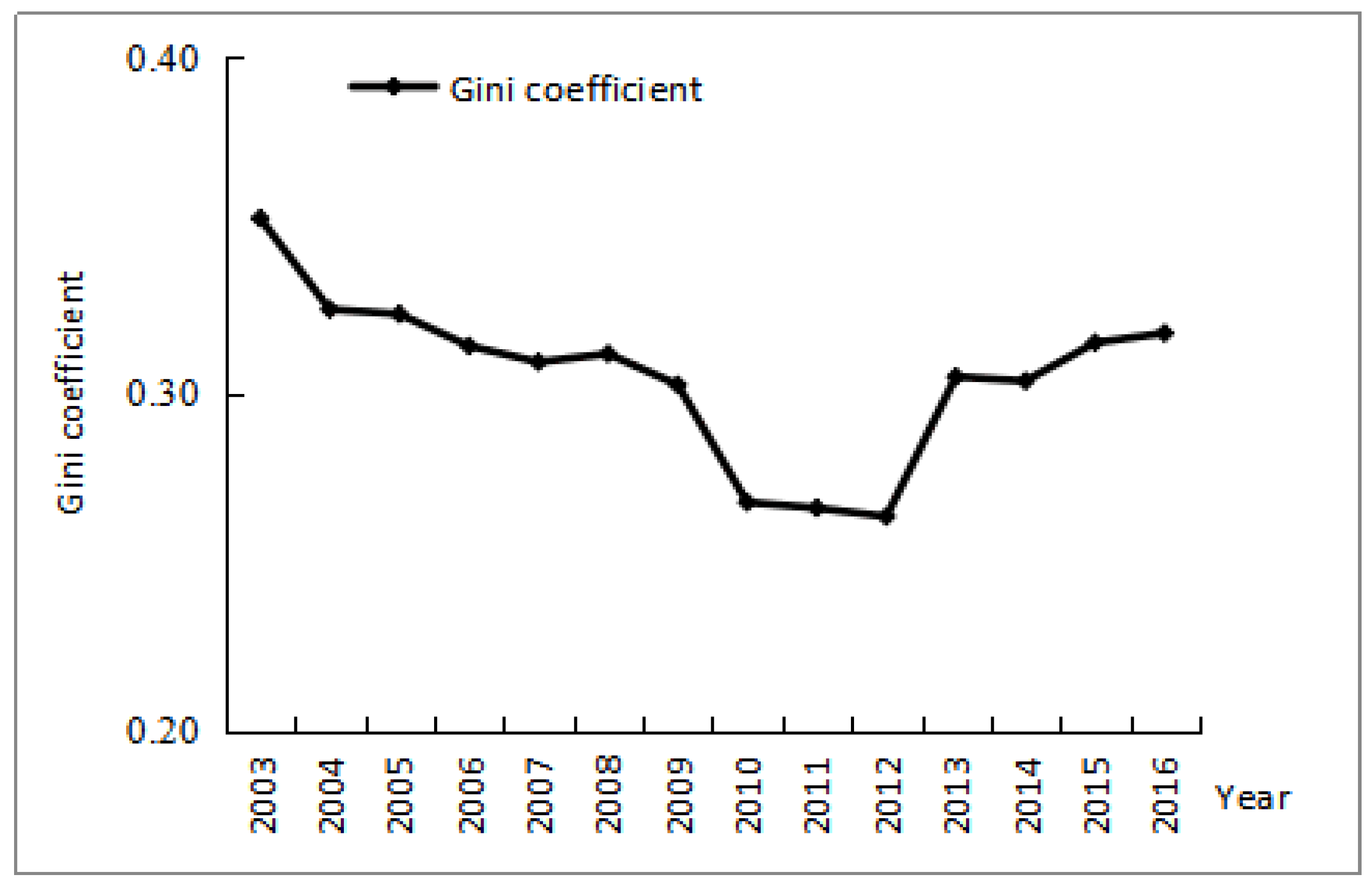
3.5. Gini Coefficient, Ecological Support Coefficient and Economic Contributive Coefficient

The Gini coefficient from 2003 to 2016 was calculated by Formula 10, and the trend is shown in Figure 11. The Gini coefficient of carbon emissions from 2003 to 2016 was concentrated between 0.2636 and 0.3522 and was relatively average from 2010 to 2012. As a whole, the study period shows a decreasing trend followed by an increasing trend, using 2012 as the cut-off point. The Gini coefficient kept decreasing from 2003 to 2012, which indicated that, with the implementation of national policies such as Western development and the revitalization of old industrial bases in Northeast China, the synergy of regional development has been enhanced. At the same time, the implementation of various forest protection policies has promoted the continuous narrowing of the gap between the distribution of carbon emissions and carbon absorption between regions. The Gini coefficient increased slightly from 2013 to 2016, indicating a gradual widening of the gap between the regional distribution of carbon emissions and carbon absorption.

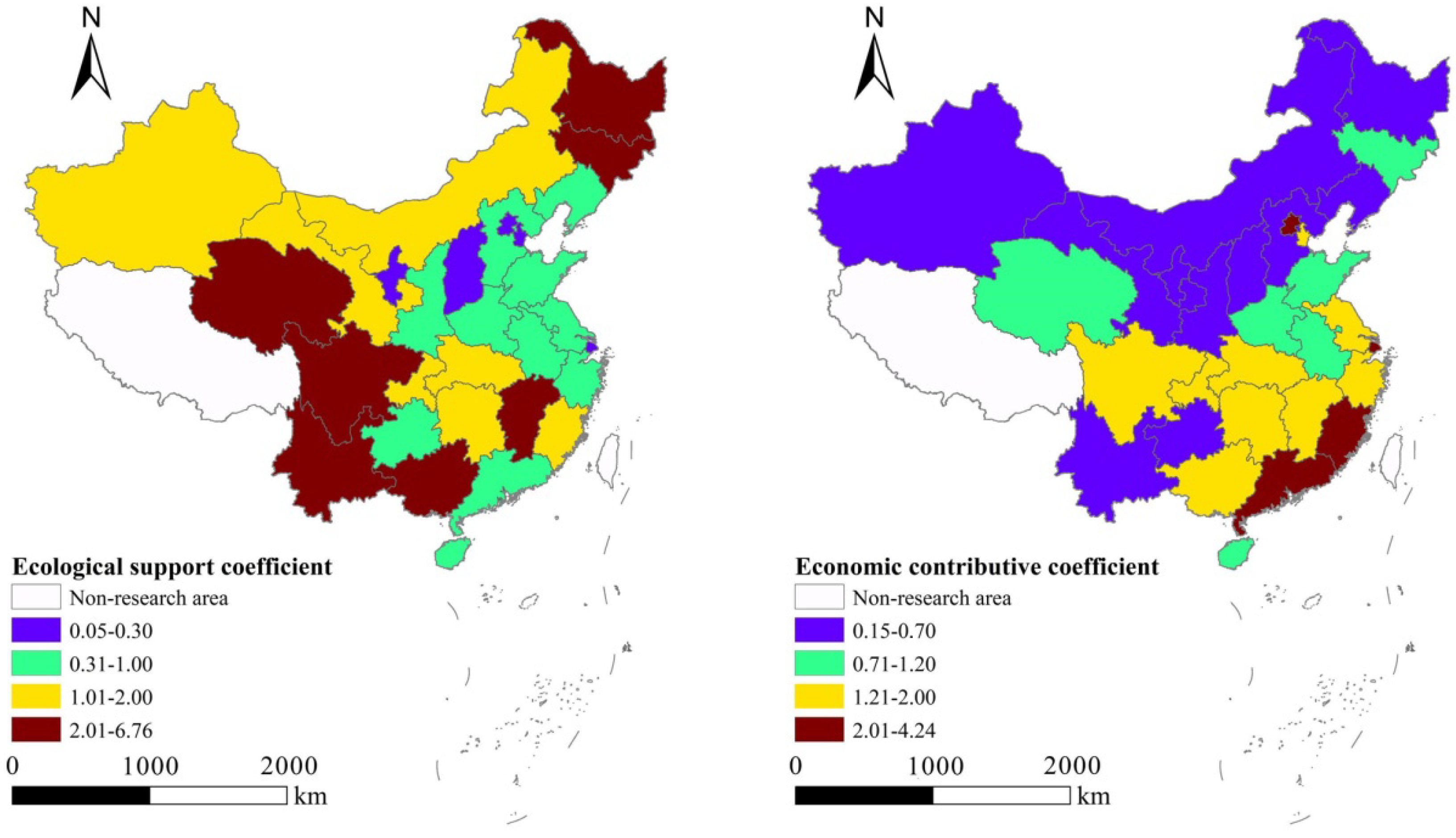
Taking 2016 as an example, the ecological support coefficient of carbon emissions in China’s provinces is analyzed. It is found in Figure 12 that the spatial distribution of the ecological support coefficient is quite different. Inner Mongolia, Heilongjiang, Jilin, Fujian, Jiangxi, Hubei, Hunan, Guangxi, Chongqing, Sichuan, Yunnan, Gansu, Qinghai, Xinjiang and 14 other provinces exceeded 1.0, and the highest was Qinghai at 6.76. The ecological support coefficients in Northeastern and Southwestern China are generally high, most of which are above 2.0. This shows that the main grain-producing areas and forest-rich areas have a high carbon sink capacity and relatively low carbon emission intensity. The ecological support coefficients of Beijing, Tianjin, Shanxi, Shanghai, Ningxia, etc. are lower than 0.3, causing inequity. This shows that the low carbon sink level of the above regions struggles to offset the carbon emissions generated, causing other regions to bear the burden. The ecological and environmental impacts caused by the greenhouse effect are disproportionate to the carbon emissions.

Figure 12 shows that the economic contributive coefficient is between 0.15 and 4.24. Beijing’s economic contributive coefficient is the highest at 4.24. Shanxi’s is the lowest at 0.15. This shows that the economic contribution rate and carbon emission contribution rate of each province are in an unbalanced state, and the spatial distribution is obviously different. The overall spatial characteristics are that the economic contributive coefficients of the Beijing-Tianjin region, the Yangtze River Delta, the two lakes and the Guangdong region are high, which indicates that the above regions have a higher economic development efficiency and energy utilization efficiency and stronger carbon productivity. Hebei, Shanxi, Inner Mongolia, Liaoning, Heilongjiang, Guizhou, Shaanxi, Gansu, Ningxia and Xinjiang are all below 0.7, along with most of these are western and northeastern provinces, which are important areas that cause inequity. The above regional economic development efficiency and energy utilization efficiency are low. As a result of generating a certain percentage of carbon emissions, the regional GDP that matches the carbon emissions has not been harvested.

According to the 2016 economic contributive coefficient and ecological support coefficient, the divisions into different evaluation matrices are shown in

Table 3. Classification results of the economic contributive coefficient and ecological carrying capacity.

Evaluation Coefficient	ESC > 1	ESC < 1
ECC > 1	JL, FJ, JX, HN, HB, GX, CQ, SC, YN	BJ, TJ, SH, JS, ZJ, HA, GD, HI
ECC < 1	IM, HL, GS, QH, XJ	HE, SX, LN, AH, SD, SN, NX, GZ

.

From Table 3, it can be seen that ECC > 1 and ESC > 1 accounted for 30% of the study area. Jilin, Fujian, Jiangxi, Hunan, Hubei, Guangxi, Chongqing, Sichuan, Yunnan, etc. have a moderate level of economic development compared with the other provinces. These provinces have a relatively high economic development efficiency and high carbon ecological capacity.

There are eight provinces in the areas of ECC > 1 and ESC < 1, accounting for 26.67% of the research area. Beijing, Tianjin, Shanghai, Jiangsu, Zhejiang, Guangdong, etc. have higher levels of economic development. Their ecological support coefficients are low, and from an ecological perspective, that has harmed the interests of other regions.

Regions with ECC < 1 and ESC > 1 account for five provinces. The economic development of Inner Mongolia, Heilongjiang, Gansu, Qinghai and Xinjiang and, in some other more sparsely populated areas, is relatively backwards, and the economic contributive coefficient is low, but the ecological support coefficient is high. Either the area of crop planting is extensive or the woodland and grassland are rich in resources and the carbon absorption is high. From an ecological perspective, that contributes to other regions.

Other provinces are “too-low” areas. These provinces have low ecological support coefficients and economic contributive coefficients, and their carbon emission ratios exceed the carbon sinks and GDP ratios at the same time. They are important areas that lead to unfair carbon emissions. From the perspective of economic development and ecology, these regions have harmed the interests of other regions.

4. Conclusions

During the study period, the provinces with rapid growth and faster growth carbon emissions nationwide were concentrated in the west and the middle reaches of the Yellow River. Slow growth and slower growth provinces are concentrated in the northwest, southwest, southern coastal regions and the northeast. The provinces with rapid growth and faster growth carbon absorption throughout the country are concentrated in the middle reaches of the Yellow River and the northern coastal areas. The provinces with slow growth and slower growth are concentrated in the northwestern, southwestern, south coastal and northeastern areas.

From the perspective of carbon absorption, the amount of carbon absorbed by cultivated land has increased year by year, the amount of carbon absorbed by woodland has increased slowly, with a small increase overall and the amount of carbon absorbed by grassland has continued to its decrease. The degree of spatial agglomeration of carbon absorption is obvious, forming a High-High agglomeration in Yunnan Province in 2010 and always a High-Low agglomeration in Inner Mongolia and a Low-Low agglomeration in Shanghai during the study period from 2005 to 2015.

From the perspective of carbon emissions, the emissions from construction land are the main source of total carbon emissions, and the proportion of carbon emissions from cultivated land is relatively low. The degree of spatial concentration of carbon emissions has become more and more noticeable. In 2015, a High-High Cluster area of Shanxi-Shandong-Inner Mongolia was formed.

There are obvious regional differences in the net carbon emissions. From 2005 to 2015, a Low-Low agglomeration was in Southwest China and a High-High agglomeration was in the central part of China and the Bohai Rim. By 2015, the Yunnan-Guangxi Low-Low cluster and Shanxi-Shandong High-High cluster were finally formed.

Carbon emissions are unfairly distributed, and the spatial distribution is significantly different. According to the carbon emission Gini coefficient, it was found that the regional distribution gap between carbon emissions and carbon absorption increased from 2013 to 2016. The spatial differences of the ecological support coefficient and economic contributive coefficient in 2016 were more obvious. The ecological support coefficient was relatively high in Southwest and Northeast China and low in Shanxi, Beijing and Tianjin. The highest economic contributive coefficient is in Beijing, and the main regional distribution of inequitable economic contribution is concentrated in the northeast and northwest regions.

In the apportionment of carbon emission reduction responsibility, the spatial distribution characteristics of carbon emissions should be fully considered, and the carbon emissions of each province under the perspectives of producer responsibility and consumer responsibility should be comprehensively considered. The reasonable allocation of carbon emission reduction responsibilities among provinces strengthen the collaboration of provincial and regional carbon emission reduction and promote interprovincial carbon fairness. The provinces should formulate interprovincial complementary emission reduction policies to achieve their carbon reduction targets in collaboration.

Carbon compensation should be implemented in combination with land use carbon emissions and carbon absorption, and the carbon compensation standard should be adjusted appropriately with the development of the economy and the changes of carbon emissions and absorption. The existing national standards should be followed, combined with different industries and different fields to make dynamic adjustments, and appropriately improve the carbon compensation standards. Adjusting the carbon compensation standards can improve the overall effectiveness of carbon compensation, and setting uniform standards is conducive to better control the environmental impact of carbon emissions.

Optimize the structure of land use. Reasonably control the total amount and development of construction land, rationally plan construction land, improve land use efficiency and realize the economical and intensive land uses. For developed cities, it is necessary to increase the areas of green space and rationally plan urban plant configurations to enhance the carbon sinks.

Improve the policies on carbon emissions. As the state implements policies such as the large-scale development of the western region and the revitalization of the old industrial bases in Northeast China, it has strengthened the regional development synergy. However, the regional distribution gap between carbon emissions and carbon absorption has gradually widened, indicating that the government should strictly implement various forest protection policies and quota logging systems to promote the continuous narrowing of the gap between regional carbon emissions and carbon absorption and distribution. At the same time, the protection and management of grassland ecosystems should be strengthened and cultivated land protection mechanisms established. The development of unused land and idle land and shift to land use types such as woodland, grassland and cultivated land should be encouraged.

Cultivate citizens’ low-carbon awareness. The fifth report of the United Nations Intergovernmental Panel on Climate Change (IPCC) states that human activities have caused more than half of the global warming since the 1950s. It is urgent to establish the values of low-carbon environmental protection and the responsibility of low-carbon emission reduction. It is necessary to strengthen the publicity of low-carbon life and make every citizen an advocate of this.

References

1. Wang, Y.; Yang, H.; Sun, R. Effectiveness of China’s provincial industrial carbon emission reduction and optimization of carbon emission reduction paths in “lagging regions”: Efficiency-cost analysis. J. Environ. Manag. 2020, 275, 111221. [Google Scholar] [CrossRef] [PubMed]
2. Tong, X. The Spatiotemporal Evolution Pattern and Influential Factor of Regional Carbon Emission Convergence in China. Adv. Meteorol. 2020, 2020, 4361570. [Google Scholar] [CrossRef]
3. Zhao, J.; Kou, L.; Wang, H.; He, X.; Xiong, Z.; Liu, C.; Cui, H. Carbon Emission Prediction Model and Analysis in the Yellow River Basin Based on a Machine Learning Method. Sustainability 2022, 14, 6153. [Google Scholar] [CrossRef]
4. Chuai, X.; Huang, X.; Wang, W.; Zhao, R.; Zhang, M.; Wu, C. Land use, total carbon emissions change and low carbon land management in Coastal Jiangsu, China. J. Clean. Prod. 2015, 103, 77–86. [Google Scholar] [CrossRef]
5. Ogle, S.M.; Domke, G.; Kurz, W.A.; Rocha, M.T.; Huffman, T.; Swan, A.; Smith, J.E.; Woodall, C.; Krug, T. Delineating managed land for reporting national greenhouse gas emissions and removals to the United Nations framework convention on climate change. Carbon Balance Manag. 2018, 13, 1–13. [Google Scholar] [CrossRef] [PubMed]
6. Zhao, J.; Shahbaz, M.; Dong, X.C.; Dong, K.Y. How does financial risk affect global CO2 emissions? The role of technological innovation. Technol. Forecast. Soc. Change 2021, 168, 120751. [Google Scholar] [CrossRef]
7. Laamrani, A.; Voroney, P.R.; Gillespie, A.W.; Chehbouni, A. Development of a Land Use Carbon Inventory for Agricultural Soils in the Canadian Province of Ontario. Land 2021, 10, 765. [Google Scholar] [CrossRef]
8. Zuo, J.; Zhong, Y.; Yang, Y.; Fu, C.; He, X.; Bao, B.; Qian, F. Analysis of carbon emission, carbon displacement and heterogeneity of Guangdong power industry. Energy Rep. 2022, 8, 438–450. [Google Scholar] [CrossRef]
9. Carpio, A.; Ponce-Lopez, R.; Lozano-García, D.F. Urban form, land use, and cover change and their impact on carbon emissions in the Monterrey Metropolitan area, Mexico. Urban Clim. 2021, 39, 100947. [Google Scholar] [CrossRef]
10. Lai, S.; Lu, J.; Luo, X.; Ge, J. Carbon emission evaluation model and carbon reduction strategies for newly urbanized areas. Sustain. Prod. Consum. 2022, 31, 13–25. [Google Scholar] [CrossRef]
11. Lv, T.; Hu, H.; Zhang, X.; Wang, L.; Fu, S. Impact of multidimensional urbanization on carbon emissions in an ecological civilization experimental area of China. Phys. Chem. Earth Parts A/B/C 2022, 126, 103120. [Google Scholar] [CrossRef]
12. Luo, Y.; Wang, W.; Zhao, D. The impacts of carbon emission trading mechanism on the power transition pathway-taking Guangdong-Hong Kong-Macao Greater Bay Area as an example. J. Clean. Prod. 2022, 330, 129894. [Google Scholar] [CrossRef]
13. Cui, Y.; Li, L.; Chen, L.; Zhang, Y.; Cheng, L.; Zhou, X.; Yang, X. Land-use carbon emissions estimation for the Yangtze River Delta Urban Agglomeration using 1994–2016 Landsat image data. Remote Sens. 2018, 10, 1334. [Google Scholar] [CrossRef] [Green Version]
14. Viveiros, F.; Chiodini, G.; Cardellini, C.; Caliro, S.; Zanon, V.; Silva, C.; Rizzo, A.L.; Hipólito, A.; Moreno, L. Deep CO2 emitted at Furnas do Enxofre geothermal area (Terceira Island, Azores archipelago). An approach for determining CO2 sources and total emissions using carbon isotopic data. J. Volcanol. Geotherm. Res. 2020, 401, 106968. [Google Scholar] [CrossRef]
15. Zhang, C.-Y.; Zhao, L.; Zhang, H.; Chen, M.-N.; Fang, R.-Y.; Yao, Y.; Zhang, Q.-P.; Wang, Q. Spatial-temporal characteristics of carbon emissions from land use change in Yellow River Delta region, China. Ecol. Indic. 2022, 136, 108623. [Google Scholar] [CrossRef]
16. Fan, J.; Zhou, L.; Zhang, Y.; Shao, S.; Ma, M. How does population aging affect household carbon emissions? Evidence from Chinese urban and rural areas. Energy Econ. 2021, 100, 105356. [Google Scholar] [CrossRef]
17. Zhang, W.J.; Xu, H.Z. Effects of land urbanization and land finance on carbon emissions: A panel data analysis for Chinese provinces. Land Use Policy 2017, 63, 493–500. [Google Scholar] [CrossRef] [Green Version]
18. Zhou, Y.; Chen, M.X.; Tang, Z.P.; Mei, Z.A. Urbanization, land use change, and carbon emissions: Quantitative assessments for city-level carbon emissions in Beijing-Tianjin-Hebei region. Sustain. Cities Soc. 2021, 66, 102701. [Google Scholar] [CrossRef]
19. Duan, H.; Zhang, Y.; Zhao, J.; Bian, X. Carbon footprint analysis of farmland ecosystem in China. J. Soil Water Conserv. 2011, 25, 203–208. [Google Scholar]
20. Shi, H.; Mu, X.; Zhang, Y.; Lu, M. Effects of different land use patterns on carbon emission in Guangyuan city of Sichuan province. Bull. Soil Water Conserv. 2012, 32, 101. [Google Scholar]
21. Xie, H.; Chen, X.; Lin, K.; Hu, A. The ecological footprint analysis of fossil energy and electricity. Acta Ecol. Sin. 2008, 28, 1729–1735. [Google Scholar]
22. Yang, G.; Chen, Y. China’s agriculture carbon sink estimation and its coupling analysis with agricultural economy development. China Popul. Resour. Environ. 2016, 26, 171–176. [Google Scholar]
23. Ding, B.; Yang, S.; Zhao, Y. Study on spatio-temporal characteristics and decoupling effect of carbon emission from cultivated land resource utilization in China. China Land Sci. 2019, 22, 45–54. [Google Scholar]
24. West, T.O.; Marland, G. A synthesis of carbon sequestration, carbon emissions, and net carbon flux in agriculture: Comparing tillage practices in the United States. Agric. Ecosyst. Environ. 2002, 91, 217–232. [Google Scholar] [CrossRef]
25. Ze-yuan, X.; Jiang, Z. Decomposition model and empirical study of carbon emissions for China, 1995–2004. China Popul. Resour. Environ. 2006, 6, 29. [Google Scholar]
26. Lu, H.; Shi, J. Reconstruction and analysis of temporal and spatial variations in surface soil moisture in China using remote sensing. Chin. Sci. Bull. 2012, 57, 2824–2834. [Google Scholar] [CrossRef] [Green Version]
27. Griffith, D.A. Spatial Econometrics: Methods and Models; Taylor & Francis: Abingdon, UK, 1989. [Google Scholar]
28. Chuai, X.; Huang, X.; Wang, W.; Wen, J.; Chen, Q.; Peng, J. Spatial econometric analysis of carbon emissions from energy consumption in China. J. Geogr. Sci. 2012, 22, 630–642. [Google Scholar] [CrossRef]
29. Bai, J.; Li, S.; Kang, Q.; Wang, N.; Guo, K.; Wang, J.; Cheng, J. Spatial Spillover Effects of Renewable Energy on Carbon Emissions in Less-developed Areas of China. Environ. Sci. Pollut. Res. 2022, 29, 19019–19032. [Google Scholar] [CrossRef]
30. Groot, L. Carbon lorenz curves. Resour. Energy Econ. 2010, 32, 45–64. [Google Scholar] [CrossRef]
31. Lu, J.; Huang, X.; Dai, L.; Chen, Z.; Li, Y. Spatio-temporal scale analysis on the equality of energy consumption carbon emission distribution in China. J. Nat. Resour. 2012, 27, 2006–2017. [Google Scholar]
32. Gini, C. Measurement of inequality of incomes. Econ. J. 1921, 31, 124–126. [Google Scholar] [CrossRef]
33. Yuan, S.; Tang, Y. Spatial differentiation of land use carbon emission in the Yangtze River economic belt based on low carbon perspective. Econ. Geogr. 2019, 39, 190–198. [Google Scholar]
Figure 1. The research framework of this paper.
Sustainability 14 07627 g001
Figure 2. The land cover and land use map of China from 2005 to 2015.
Sustainability 14 07627 g002
Figure 3. Lorenz Curve.
Sustainability 14 07627 g003
Figure 4. Growth level of carbon emissions and total carbon absorption in provinces from 2003 to 2016.
Sustainability 14 07627 g004
Figure 5. Global Moran’s I index scatter plot for the total CO2 absorption in each province in 2005, 2010 and 2015.
Sustainability 14 07627 g005
Figure 6. Distribution of the total CO2 absorption in 2005, 2010 and 2015.
Sustainability 14 07627 g006
Figure 7. Global Moran’s I index scatter plots for the total CO2 emissions in 2005, 2010 and 2015.
Sustainability 14 07627 g007
Figure 8. Distribution of the total CO2 emissions in 2005, 2010 and 2015.
Sustainability 14 07627 g008
Figure 9. Global Moran’s I index scatter plots for the total carbon emissions in 2005, 2010 and 2015.
Sustainability 14 07627 g009
Figure 10. Distribution of the total carbon emissions in 2005, 2010 and 2015.
Sustainability 14 07627 g010
Figure 11. Trend of the Gini coefficient.
Sustainability 14 07627 g011
Figure 12. Spatial distribution of China’s provincial ecological carrying capacity coefficient and economic contributive coefficient in 2016.
Sustainability 14 07627 g012