
Cluster-Based Routing Protocol with Static Hub (CRPSH) for WSN-Assisted IoT Networks

 , ,
, ,  ,
,  and
and
Abstract
1. Introduction
2. Literature Review
3. System Model
3.1. Assumptions
3.2. Energy Consumption Model
4. Proposed Protocol
4.1. Peer Discovery
| Algorithm 1 Peer Discovery |
| INPUT: Peer Discovery Control Packet |
| OUTPUT: Return Hub Adjacency Matrix |
| 1: = where = { w : w are the Peer/ Neighbor Device of the device }; |
| 2: = where is the Peer/ Neighbor table of the IoT Device ; |
| 3: is the remaining energy level of the IoT Device ; |
| 4: Initially = False; |
| 5: Set = True when the the IoT Device sends the packet; |
| 6: is the location of the IoT Device ; |
| 7: Device receives the control packet : <, , > from the Device ; |
| 8: if ∉ then |
| 9: = ⋃ ; |
| 10: Update with <, , >; |
| 11: if == false then |
| 12: ← True; |
| 13: Broadcast : <, >; ▹ Broadcast packet; |
| 14: else |
| 15: Discard the packet |
| 16: end if |
| 17: Discard the packet |
| 18: end if |
| 19: Device receives the control packet : < , , , > from the Device ; |
| 20: if = then |
| 21: if ∉ then |
| 22: = ⋃; |
| 23: if == then |
| 24: Update peer adjacency matrix using ; |
| 25: else |
| 26: Forward the packet to the selected relay node; |
| 27: end if |
| 28: Discard the packet |
| 29: end if |
| 30: Discard the packet |
| 31: end if |
4.2. Cluster Head Selection and Cluster Formation
- 1.
- Two CHs should not be located adjacent to one another.
- Let Device be selected as CH;
- is a set peer device of the Device ;
- if () then
- Device cannot be CH.
- end if
- 2.
- Each CH’s residual energy, , should be larger than the threshold value.
- 3.
- Each cluster head should have a peer count of at least /2.
- Let k be the number of devices in the network and c denote the ideal number of CHs.
- Then, = (k-c)/c. In the ideal situation, is the average number of devices in a cluster. So each CH should satisfy ⩾ /2.
| Algorithm 2 Cluster Head Announcement |
| INPUT: Hub sends packet to the Cluster Heads. |
| OUTPUT: Cluster Heads send packet to the hub. |
| 1: is a collection of sensor devices that form the route between node k and the hub. |
| 2: Each relay device maintains a routing table with two columns: cluster head and , which is initialized to . |
| 3: Device receives the packet from the Device ; |
| 4: : < , , , > |
| 5: if ( == ) then |
| 6: Forward the ACK Packet : < , , > towards the hub. |
| 7: else |
| 8: if ( Route (CH)) then |
| 9: Update the by updating cluster head as and as ; |
| 10: Broadcast : < , , , > packet. |
| 11: else |
| 12: Discard the packet; |
| 13: end if |
| 14: end if |
| 15: : < , , > |
| 16: if () then |
| 17: if () then |
| 18: ; |
| 19: else |
| 20: Find the of CH from the ; |
| 21: Forward the ACK Packet : < , , > towards the hub. |
| 22: end if |
| 23: else |
| 24: Drop the packet. |
| 25: end if |
| Algorithm 3 Cluster Formation |
| INPUT: CH sends packet packet to the CMs. |
| OUTPUT: CH sends to the hub and TDMA slots to each CM. |
| 1: Device receives the packet from the Device , where |
| 2: : < , > |
| 3: Device selects the CH with the maximum received signal intensity as its CH after receiving all packets. |
| 4: Device sends the packet to the selected CH. |
| 5: Device receives the packet from the Device , where |
| 6: : < , , > |
| 7: if ( == ) then |
| 8: ; |
| 9: Device sends the to the hub after receiving all the packets. |
| 10: Device sends the TDMA slots to each CM. |
| 11: else |
| 12: Discard the packet. |
| 13: end if |
4.3. Data Transmission
4.4. Re-Clustering and Rerouting
5. Simulation Results
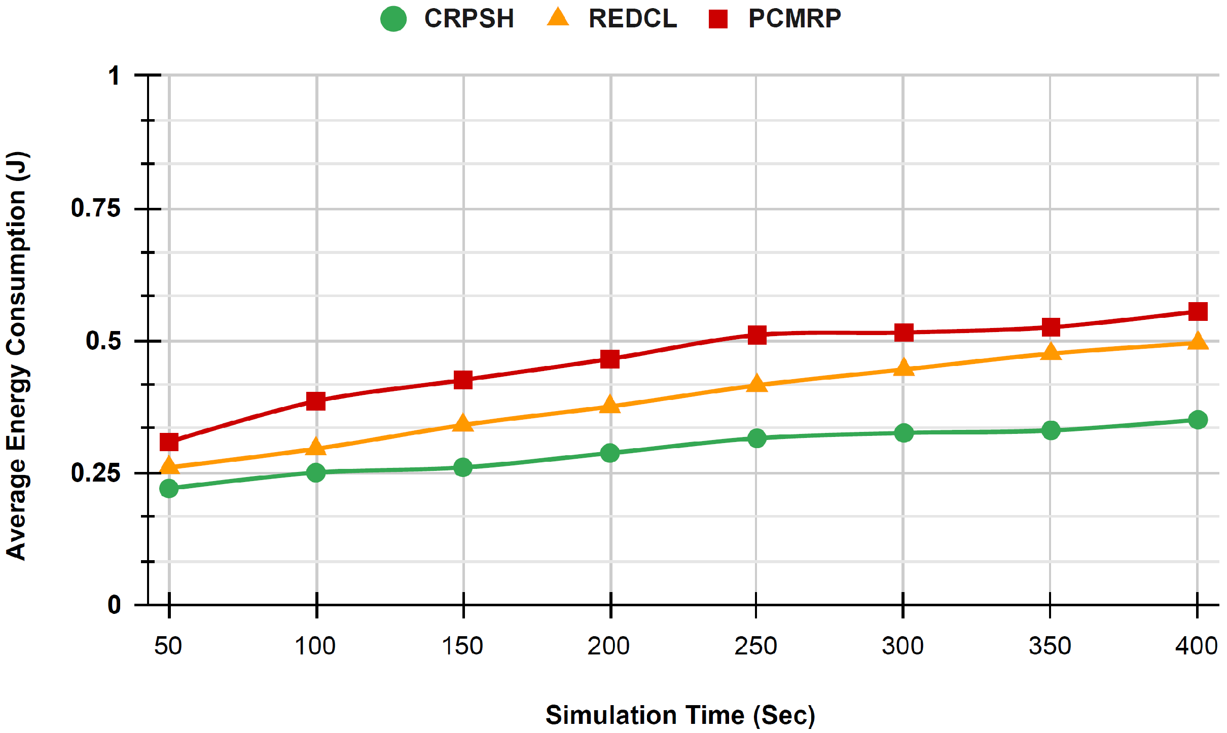
5.1. Average Energy Consumption
5.2. Average End-to-End Delay
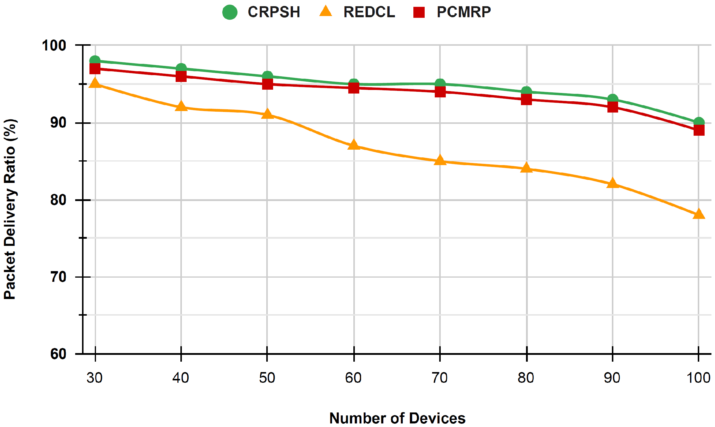
5.3. Packet Delivery Ratio
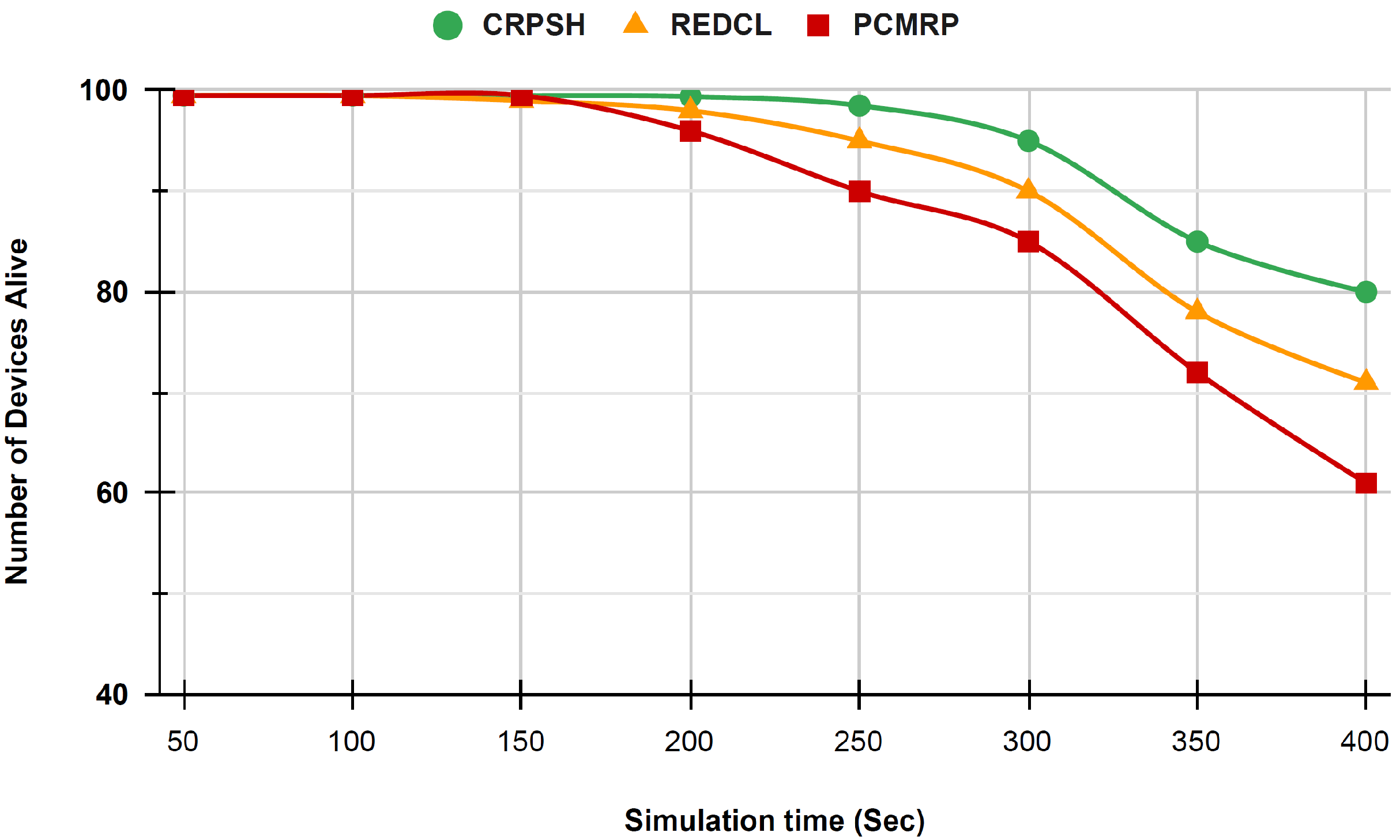
5.4. Network Lifetime
6. Conclusions
Author Contributions
Funding
Institutional Review Board Statement
Informed Consent Statement
Data Availability Statement
Conflicts of Interest
Abbreviations
| CH | Cluster Heads |
| CM | Cluster Members |
| LLNs | Low-power and Lossy networks |
| CRPSH | Cluster-based Routing Protocol with Static Hub |
| IoT | Internet of Things |
| ANPIREQ | AN Position Information Request packet |
| ANPIRES | AN Location Information Response |
| QDD | Quadtree-based Routing Protocol |
| CBRP | Centroid-based Routing Protocol |
| SCBC | Sector-Chain-Based Clustering Routing Protocol |
| SCH | Secondary Cluster Head |
| BS | Base Station |
| HRPM | Hierarchical Rendezvous Point Multicast |
| HGMR | Hierarchical Geographic Multicast Routing Protocol |
| GMCAR | Grid-based Multipath Routing Protocol |
| LGH | Local Grid Head |
| TDMA | Time Division Multiple Access |
| GBRR | Grid-Based Reliable Routing |
| MSGR | Grid-Based Sustainable Routing Protocol |
| PCMRP | Passive cluster-based multipath routing protocol for WSNs |
| REDCL | Reliable and energy-efficient data collection for WSNs |
| Energy required for an embedded circuit to receive or transmit a signal of one bit | |
| Amplifier energy consumption to preserve radio reliable transmission |
References
- Sarkar, S.; Debnath, A. Green IoT: Design Goals, Challenges and Energy Solutions. In Proceedings of the 2021 6th International Conference on Communication and Electronics Systems (ICCES), Coimbatre, India, 8–10 July 2021; pp. 637–642. [Google Scholar]
- Verma, G.; Prakash, S. A Comparative Study Based on Different Energy Saving Mechanisms Based on Green Internet of Things (GIoT). In Proceedings of the 2020 8th International Conference on Reliability, Infocom Technologies and Optimization (Trends and Future Directions) (ICRITO), Noida, India, 4–5 June 2020; pp. 659–666. [Google Scholar]
- Al-Turjman, F.M.; Zahmatkesh, H.; Shahroze, R. An overview of security and privacy in smart cities’ IoT communications. Trans. Emerg. Telecommun. Technol. 2022, 33, e3677. [Google Scholar] [CrossRef]
- Deebak, B.D.; Al-Turjman, F.M. Lightweight authentication for IoT/Cloud-based forensics in intelligent data computing. Future Gener. Comput. Syst. 2021, 116, 406–425. [Google Scholar] [CrossRef]
- Lenka, R.K.; Rath, A.K.; Sharma, S. Building Reliable Routing Infrastructure for Green IoT Network. IEEE Access 2019, 7, 129892–129909. [Google Scholar] [CrossRef]
- Lenka, R.K.; Rath, A.K.; Tan, Z.; Sharma, S.; Puthal, D.; Simha, N.V.R.; Prasad, M.; Raja, R.; Tripathi, S.S. Building Scalable Cyber-Physical-Social Networking Infrastructure Using IoT and Low Power Sensors. IEEE Access 2018, 6, 30162–30173. [Google Scholar] [CrossRef]
- Sourailidis, D.; Koutsiamanis, R.A.; Papadopoulos, G.Z.; Barthel, D.; Montavont, N. RFC 6550: On Minimizing the Control Plane Traffic of RPL-based Industrial Networks. In Proceedings of the 2020 IEEE 21st International Symposium on “A World of Wireless, Mobile and Multimedia Networks” (WoWMoM), Cork, Ireland, 31 August–3 September 2020; pp. 439–444. [Google Scholar]
- Al-Turjman, F.; Deebak, B.D. Seamless Authentication: For IoT-Big Data Technologies in Smart Industrial Application Systems. IEEE Trans. Ind. Informatics 2021, 17, 2919–2927. [Google Scholar] [CrossRef]
- Al-Turjman, F.; Altrjman, C.; Din, S.; Paul, A. Energy monitoring in IoT-based ad hoc networks: An overview. Comput. Electr. Eng. 2019, 76, 133–142. [Google Scholar] [CrossRef]
- Mohapatra, K.; Lenka, R.K.; Sharma, S. A Survey on Classical and Optimized Hierarchical Routing Protocols for IoT and WSN. In Proceedings of the 2021 6th International Conference on Signal Processing, Computing and Control (ISPCC), Solan, India, 7–9 October 2021; pp. 620–624. [Google Scholar]
- Pratik, T.; Lenka, R.K.; Nayak, G.K.; Kumar, A. An Architecture to Support Interoperability in IoT Devices. In Proceedings of the 2018 International Conference on Advances in Computing, Communication Control and Networking (ICACCCN), Greater Noida, India, 12–13 October 2018; pp. 705–710. [Google Scholar]
- Lenka, R.K.; Barik, R.K.; Das, N.K.; Agarwal, K.; Mohanty, D.; Vipsita, S. PSPS: An IoT based predictive smart parking system. In Proceedings of the 2017 4th IEEE Uttar Pradesh Section International Conference on Electrical, Computer and Electronics (UPCON), Mathura, India, 26–28 October 2017; pp. 311–317. [Google Scholar]
- Lenka, R.K.; Aggarwal, A.; Rath, A.; Sharma, S. Cluster-based rendezvous routing protocol for wireless sensor network. In Proceedings of the 2017 International Conference on Computing, Communication and Automation (ICCCA), Greater Noida, India, 5–6 May 2017; pp. 748–752. [Google Scholar]
- Lenka, R.K.; Rath, A.K.; Sharma, S. Routing Protocols in WSN Assisted IoT Infrastructure—A Review. In Proceedings of the 2019 International Conference on Intelligent Computing and Remote Sensing (ICICRS), Bhubaneswar, India, 19–20 July 2019; pp. 1–6. [Google Scholar]
- Liu, X. Atypical hierarchical routing protocols for wireless sensor networks: A review. IEEE Sens. J. 2015, 15, 5372–5383. [Google Scholar] [CrossRef]
- Natarajan, Y.; Srihari, K.; Dhiman, G.; Chandragandhi, S.; Gheisari, M.; Liu, Y.; Lee, C.C.; Singh, K.K.; Yadav, K.; Alharbi, H.F. An IoT and machine learning-based routing protocol for reconfigurable engineering application. IET Commun. 2022, 16, 464–475. [Google Scholar] [CrossRef]
- Sood, T.; Sharma, K. P-LUET: A Prolong Lines of Uniformity Based Enhanced Threshold Algorithm for Heterogeneous Wireless Sensor Network Enabled Internet of Things Framework. Wirel. Pers. Commun. 2021, 120, 2935–2970. [Google Scholar] [CrossRef]
- Rahman, G.M.E.; Wahid, K.A. LDCA: Lightweight Dynamic Clustering Algorithm for IoT-Connected Wide-Area WSN and Mobile Data Sink Using LoRa. IEEE Internet Things J. 2022, 9, 1313–1325. [Google Scholar] [CrossRef]
- Karthick, K.; Asokan, R. Mobility Aware Quality Enhanced Cluster Based Routing Protocol for Mobile Ad-Hoc Networks Using Hybrid Optimization Algorithm. Wirel. Pers. Commun. 2021, 119, 3063–3087. [Google Scholar] [CrossRef]
- Shi, K.; Liu, C.; Sun, Z.; Yue, X. Coupled orbit-attitude dynamics and trajectory tracking control for spacecraft electromagnetic docking. Appl. Math. Model. 2022, 101, 553–572. [Google Scholar] [CrossRef]
- Hamida, E.B.; Chelius, G. A line-based data dissemination protocol for wireless sensor networks with mobile sink. In Proceedings of the 2008 IEEE International Conference on Communications, Beijing, China, 19–23 May 2008; pp. 2201–2205. [Google Scholar]
- Mohapatra, H.; Rath, A.K. IoE based framework for smart agriculture. J. Ambient Intell. Humaniz. Comput. 2022, 13, 407–424. [Google Scholar] [CrossRef]
- Mohapatra, H.; Rath, A.K. An IoT based efficient multi-objective real-time smart parking system. Int. J. Sens. Netw. 2021, 37, 219–232. [Google Scholar] [CrossRef]
- Mohapatra, H.; Rath, A.K. A fault tolerant routing scheme for advanced metering infrastructure: An approach towards smart grid. Clust. Comput. 2021, 24, 2193–2211. [Google Scholar] [CrossRef]
- Tunca, C.; Isik, S.; Donmez, M.Y.; Ersoy, C. Ring routing: An energy-efficient routing protocol for wireless sensor networks with a mobile sink. IEEE Trans. Mob. Comput. 2014, 14, 1947–1960. [Google Scholar] [CrossRef]
- Shin, J.H.; Kim, J.; Park, K.; Park, D. Railroad: Virtual infrastructure for data dissemination in wireless sensor networks. In Proceedings of the 2nd ACM International Workshop on Performance Evaluation of Wireless Ad Hoc, Sensor, and Ubiquitous Networks, Montreal, QC, Canada, 10–13 October 2005; pp. 168–174. [Google Scholar]
- Sharma, S.; Puthal, D.; Jena, S.K.; Zomaya, A.Y.; Ranjan, R. Rendezvous based routing protocol for wireless sensor networks with mobile sink. J. Supercomput. 2017, 73, 1168–1188. [Google Scholar] [CrossRef]
- Mir, Z.H.; Ko, Y.B. A quadtree-based data dissemination protocol for wireless sensor networks with mobile sinks. In Proceedings of the IFIP International Conference on Personal Wireless Communications, Albacete, Spain, 20–22 September 2006; Springer: Berlin/Heidelberg, Germany, 2006; pp. 447–458. [Google Scholar]
- Shen, J.; Wang, A.; Wang, C.; Hung, P.C.; Lai, C.F. An efficient centroid-based routing protocol for energy management in WSN-assisted IoT. IEEE Access 2017, 5, 18469–18479. [Google Scholar] [CrossRef]
- Tan, N.D.; Viet, N.D. SCBC: Sector-chain based clustering routing protocol for energy efficiency in heterogeneous wireless sensor network. In Proceedings of the 2015 International Conference on Advanced Technologies for Communications (ATC), Ho Chi Minh City, Vietnam, 14–16 October 2015; pp. 314–319. [Google Scholar]
- Heinzelman, W.B.; Chandrakasan, A.P.; Balakrishnan, H. An application-specific protocol architecture for wireless microsensor networks. IEEE Trans. Wirel. Commun. 2002, 1, 660–670. [Google Scholar] [CrossRef]
- Gnanambigai, J.; Rengarajan, D.N.; Anbukkarasi, K. Leach and its descendant protocols: A survey. Int. J. Commun. Comput. Technol. 2012, 1, 15–21. [Google Scholar]
- Biradar, R.V.; Sawant, S.; Mudholkar, R.; Patil, V. Multihop routing in self-organizing wireless sensor networks. Int. J. Comput. Sci. Issues 2011, 8, 155. [Google Scholar]
- Qiang, T.; Bingwen, W.; Zhicheng, D. MS-Leach: A routing protocol combining multi-hop transmissions and single-hop transmissions. In Proceedings of the 2009 Pacific-Asia Conference on Circuits, Communications and Systems, Chengdu, China, 16–17 May 2009; pp. 107–110. [Google Scholar]
- Farooq, M.O.; Dogar, A.B.; Shah, G.A. MR-LEACH: Multi-hop routing with low energy adaptive clustering hierarchy. In Proceedings of the 2010 Fourth International Conference on Sensor Technologies and Applications, Venice, Italy, 18–25 July 2010; pp. 262–268. [Google Scholar]
- Sanchez, J.A.; Ruiz, P.M.; Stojmenovic, I. GMR: Geographic multicast routing for wireless sensor networks. In Proceedings of the 2006 3rd Annual IEEE Communications Society on Sensor and Ad Hoc Communications and Networks, Reston, VA, USA, 28 September 2006; Volume 1, pp. 20–29. [Google Scholar]
- Buttyán, L.; Schaffer, P. Position-based aggregator node election in wireless sensor networks. Int. J. Distrib. Sens. Netw. 2010, 6, 679205. [Google Scholar] [CrossRef]
- Akl, R.; Sawant, U. Grid-based coordinated routing in wireless sensor networks. In Proceedings of the 2007 4th IEEE Consumer Communications and Networking Conference, Las Vegas, NV, USA, 11–13 January 2007; pp. 860–864. [Google Scholar]
- Das, S.M.; Pucha, H.; Hu, Y.C. Distributed hashing for scalable multicast in wireless ad hoc networks. IEEE Trans. Parallel Distrib. Syst. 2008, 19, 347–362. [Google Scholar] [CrossRef]
- Koutsonikolas, D.; Das, S.M.; Hu, Y.C.; Stojmenovic, I. Hierarchical geographic multicast routing for wireless sensor networks. Wirel. Netw. 2010, 16, 449–466. [Google Scholar] [CrossRef]
- Banimelhem, O.; Khasawneh, S. GMCAR: Grid-based multipath with congestion avoidance routing protocol in wireless sensor networks. Ad Hoc Netw. 2012, 10, 1346–1361. [Google Scholar] [CrossRef]
- Chi, Y.P.; Chang, H.P. An energy-aware grid-based routing scheme for wireless sensor networks. Telecommun. Syst. 2013, 54, 405–415. [Google Scholar] [CrossRef][Green Version]
- Khan, A.W.; Abdullah, A.H.; Razzaque, M.A.; Bangash, J.I. VGDRA: A virtual grid-based dynamic routes adjustment scheme for mobile sink-based wireless sensor networks. IEEE Sens. J. 2014, 15, 526–534. [Google Scholar] [CrossRef]
- Jin, R.C.; Gao, T.; Song, J.Y.; Zou, J.Y.; Wang, L.D. Passive cluster-based multipath routing protocol for wireless sensor networks. Wirel. Netw. 2013, 19, 1851–1866. [Google Scholar] [CrossRef]
- Dong, M.; Ota, K.; Liu, A. RMER: Reliable and energy-efficient data collection for large-scale wireless sensor networks. IEEE Internet Things J. 2016, 3, 511–519. [Google Scholar] [CrossRef]
- Sharma, S.; Suresh, D. VGBST: A virtual grid-based backbone structure type scheme for mobile sink based wireless sensor networks. In Proceedings of the 2015 International Conference on Advanced Research in Computer Science Engineering & Technology (ICARCSET 2015), Unnao, India, 6–7 March 2015; pp. 1–5. [Google Scholar]
- Meng, X.; Shi, X.; Wang, Z.; Wu, S.; Li, C. A grid-based reliable routing protocol for wireless sensor networks with randomly distributed clusters. Ad Hoc Netw. 2016, 51, 47–61. [Google Scholar] [CrossRef]
- Sharma, S.; Puthal, D.; Tazeen, S.; Prasad, M.; Zomaya, A.Y. MSGR: A mode-switched grid-based sustainable routing protocol for wireless sensor networks. IEEE Access 2017, 5, 19864–19875. [Google Scholar] [CrossRef]
- Jung, S.M.; Han, Y.J.; Chung, T.M. The concentric clustering scheme for efficient energy consumption in the PEGASIS. In Proceedings of the 9th International Conference on Advanced Communication Technology, Gangwon, Korea, 12–14 February 2007; Volume 1, pp. 260–265. [Google Scholar]
- Xi-rong, B.; Shi, Z.; Ding-yu, X.; Zhi-tao, Q. An energy-balanced chain-cluster routing protocol for wireless sensor networks. In Proceedings of the 2010 Second International Conference on Networks Security, Wireless Communications and Trusted Computing, Wuhan, China, 24–25 April 2010; Volume 2, pp. 79–84. [Google Scholar]
- Lindsey, S.; Raghavendra, C.; Sivalingam, K.M. Data gathering algorithms in sensor networks using energy metrics. IEEE Trans. Parallel Distrib. Syst. 2002, 13, 924–935. [Google Scholar] [CrossRef]
- Chen, K.H.; Huang, J.M.; Hsiao, C.C. CHIRON: An energy-efficient chain-based hierarchical routing protocol in wireless sensor networks. In Proceedings of the 2009 Wireless Telecommunications Symposium, Prague, Czech Republic, 22–24 April 2009; pp. 1–5. [Google Scholar]
- Kim, H.S.; Han, K.J. A power efficient routing protocol based on balanced tree in wireless sensor networks. In Proceedings of the First International Conference on Distributed Frameworks for Multimedia Applications, Besancon, France, 6–9 February 2005; pp. 138–143. [Google Scholar]
- Ding, M.; Cheng, X.; Xue, G. Aggregation tree construction in sensor networks. In Proceedings of the 2003 IEEE 58th Vehicular Technology Conference. VTC 2003-Fall (IEEE Cat. No. 03CH37484), Orlando, FL, USA, 6–9 October 2003; Volume 4, pp. 2168–2172. [Google Scholar]
- Tan, H.Ö.; Körpeoǧlu, I. Power efficient data gathering and aggregation in wireless sensor networks. Acm Sigmod Rec. 2003, 32, 66–71. [Google Scholar] [CrossRef]
- Qiu, W.; Skafidas, E.; Hao, P. Enhanced tree routing for wireless sensor networks. Ad Hoc Netw. 2009, 7, 638–650. [Google Scholar] [CrossRef]
- Luo, H.; Ye, F.; Cheng, J.; Lu, S.; Zhang, L. TTDD: Two-tier data dissemination in large-scale wireless sensor networks. Wirel. Netw. 2005, 11, 161–175. [Google Scholar] [CrossRef]
- Mo, H.S.; Lee, E.; Park, S.; Kim, S.H. Virtual line-based data dissemination for mobile sink groups in wireless sensor networks. IEEE Commun. Lett. 2013, 17, 1864–1867. [Google Scholar] [CrossRef]
- Roy, N.R.; Chandra, P. Energy dissipation model for wireless sensor networks: A survey. Int. J. Inf. Technol. 2020, 12, 1343–1353. [Google Scholar] [CrossRef]


| Protocol | Classification | Mobility | Energy | Scalability | Delay |
|---|---|---|---|---|---|
| CCS [49] | Chain Based | No | Very Low | Low | Large |
| EBCRP [50] | Chain Based | No | Very Low | Low | Large |
| PEGASIS [51] | Chain Based | No | Very Low | Very Low | Very Large |
| CHIRON [52] | Chain Based | No | Moderate | Low | Small |
| BATR [53] | Tree Based | No | Low | Low | Large |
| EADAT [54] | Tree Based | No | Moderate | Low | Large |
| PEDAP [55] | Tree Based | Yes | Moderate | Low | Moderate |
| ETR [56] | Tree Based | No | Moderate | Moderate | Moderate |
| TTDD [57] | Grid Based | Yes | Very Low | Moderate | Very Large |
| PANEL [37] | Grid Based | No | Moderate | Moderate | Moderate |
| HGMR [40] | Grid Based | No | Low | High | Moderate |
| GMCARE [41] | Grid Based | No | Moderate | Moderate | Moderate |
| RRP1 [25] | Area Based | Yes | Moderate | Moderate | Moderate |
| LBDD [21] | Area Based | Yes | Moderate | Moderate | Moderate |
| VLDD [58] | Area Based | Yes | Moderate | Moderate | Large |
| RRP2 [26] | Area Based | Yes | Moderate | Moderate | Large |
| Parameter Name | Value |
|---|---|
| Network Size | m |
| Number of sensor devices | 100 |
| Data packet size | 512 bytes |
| Control packet size | 32 bytes |
| Initial energy | 1 J |
| 50 nJ/bit | |
| 10 pJ/bit/m | |
| 0.0013 pJ/bit/m | |
| 87 m | |
| 5 nJ/bit | |
| 0.2 nJ/s | |
| Simulation time | 400 s |
| MAC protocol | TMAC |
Publisher’s Note: MDPI stays neutral with regard to jurisdictional claims in published maps and institutional affiliations. |
© 2022 by the authors. Licensee MDPI, Basel, Switzerland. This article is an open access article distributed under the terms and conditions of the Creative Commons Attribution (CC BY) license (https://creativecommons.org/licenses/by/4.0/).
Share and Cite
Lenka, R.K.; Kolhar, M.; Mohapatra, H.; Al-Turjman, F.; Altrjman, C. Cluster-Based Routing Protocol with Static Hub (CRPSH) for WSN-Assisted IoT Networks. Sustainability 2022, 14, 7304. https://doi.org/10.3390/su14127304
Lenka RK, Kolhar M, Mohapatra H, Al-Turjman F, Altrjman C. Cluster-Based Routing Protocol with Static Hub (CRPSH) for WSN-Assisted IoT Networks. Sustainability. 2022; 14(12):7304. https://doi.org/10.3390/su14127304
Chicago/Turabian StyleLenka, Rakesh Kumar, Manjur Kolhar, Hitesh Mohapatra, Fadi Al-Turjman, and Chadi Altrjman. 2022. "Cluster-Based Routing Protocol with Static Hub (CRPSH) for WSN-Assisted IoT Networks" Sustainability 14, no. 12: 7304. https://doi.org/10.3390/su14127304
APA StyleLenka, R. K., Kolhar, M., Mohapatra, H., Al-Turjman, F., & Altrjman, C. (2022). Cluster-Based Routing Protocol with Static Hub (CRPSH) for WSN-Assisted IoT Networks. Sustainability, 14(12), 7304. https://doi.org/10.3390/su14127304