
GIS and Remote Sensing-Based Multi-Criteria Analysis for Delineation of Groundwater Potential Zones: A Case Study for Industrial Zones in Bangladesh

 ,
, 
 ,
,  ,
,  ,
,
Abstract
:1. Introduction
2. Materials and Methods
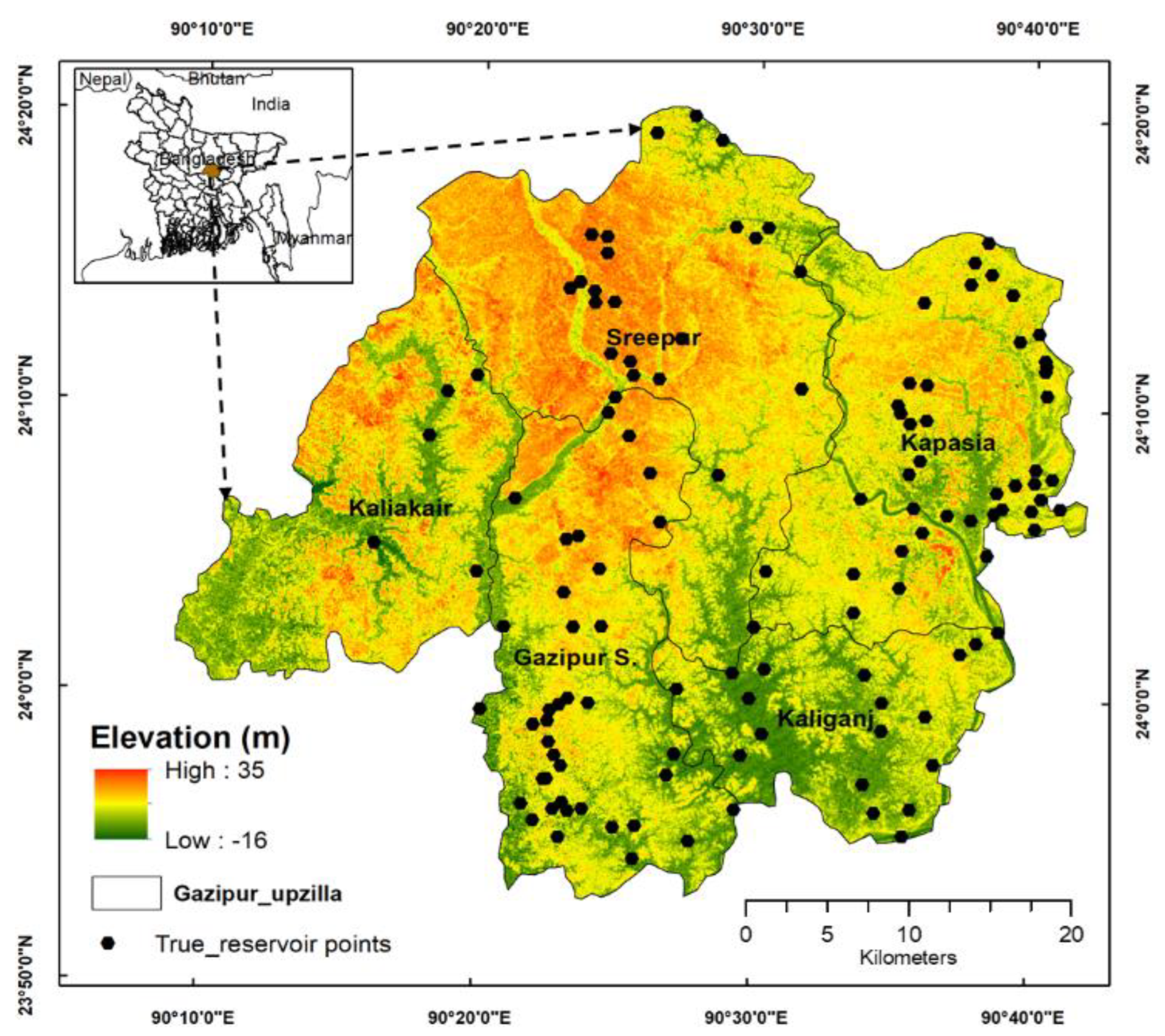
2.1. Study Area
2.2. Thematic Layers Selection
2.2.1. Slope
2.2.2. Drainage Density
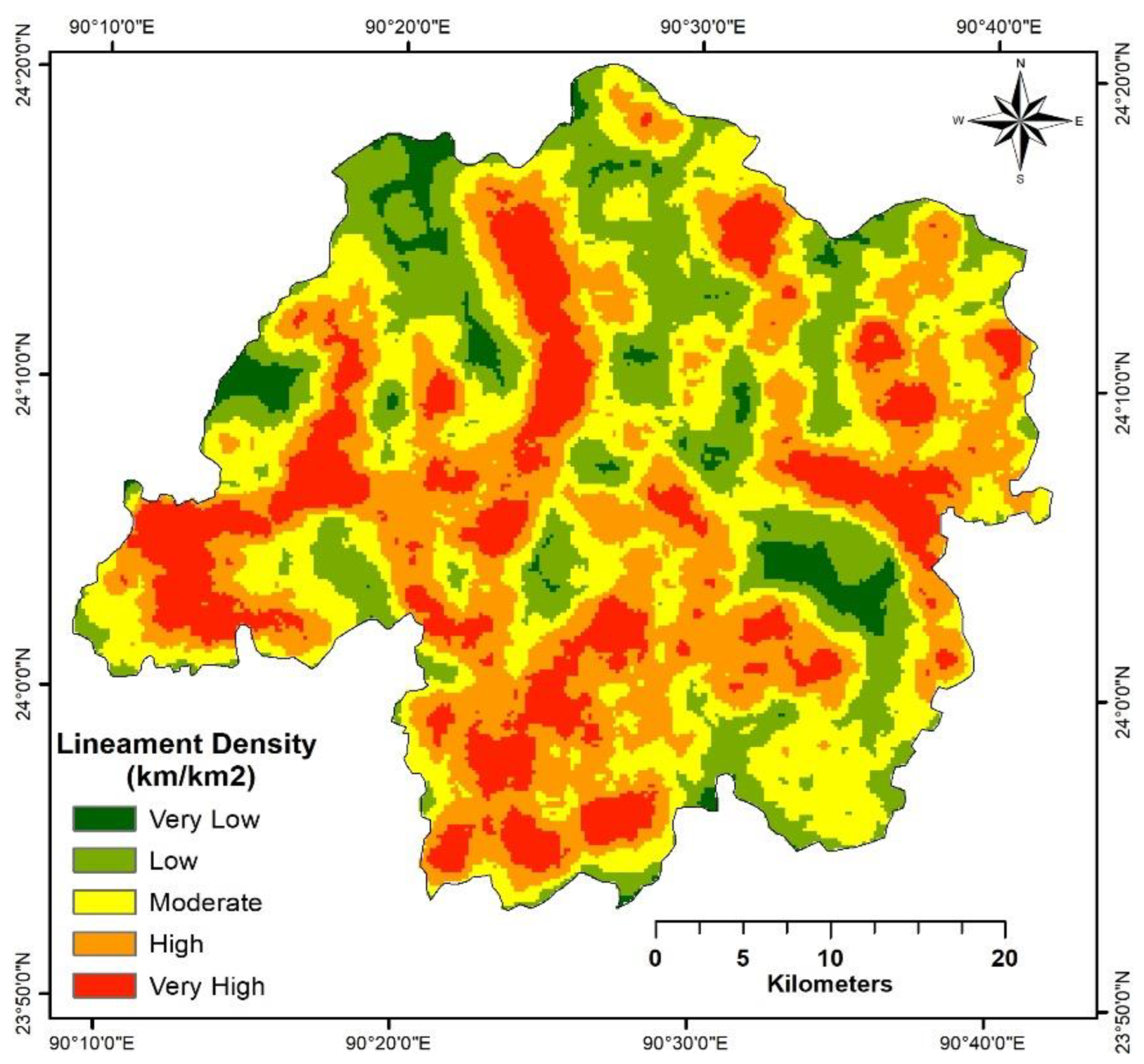
2.2.3. Lineament Density
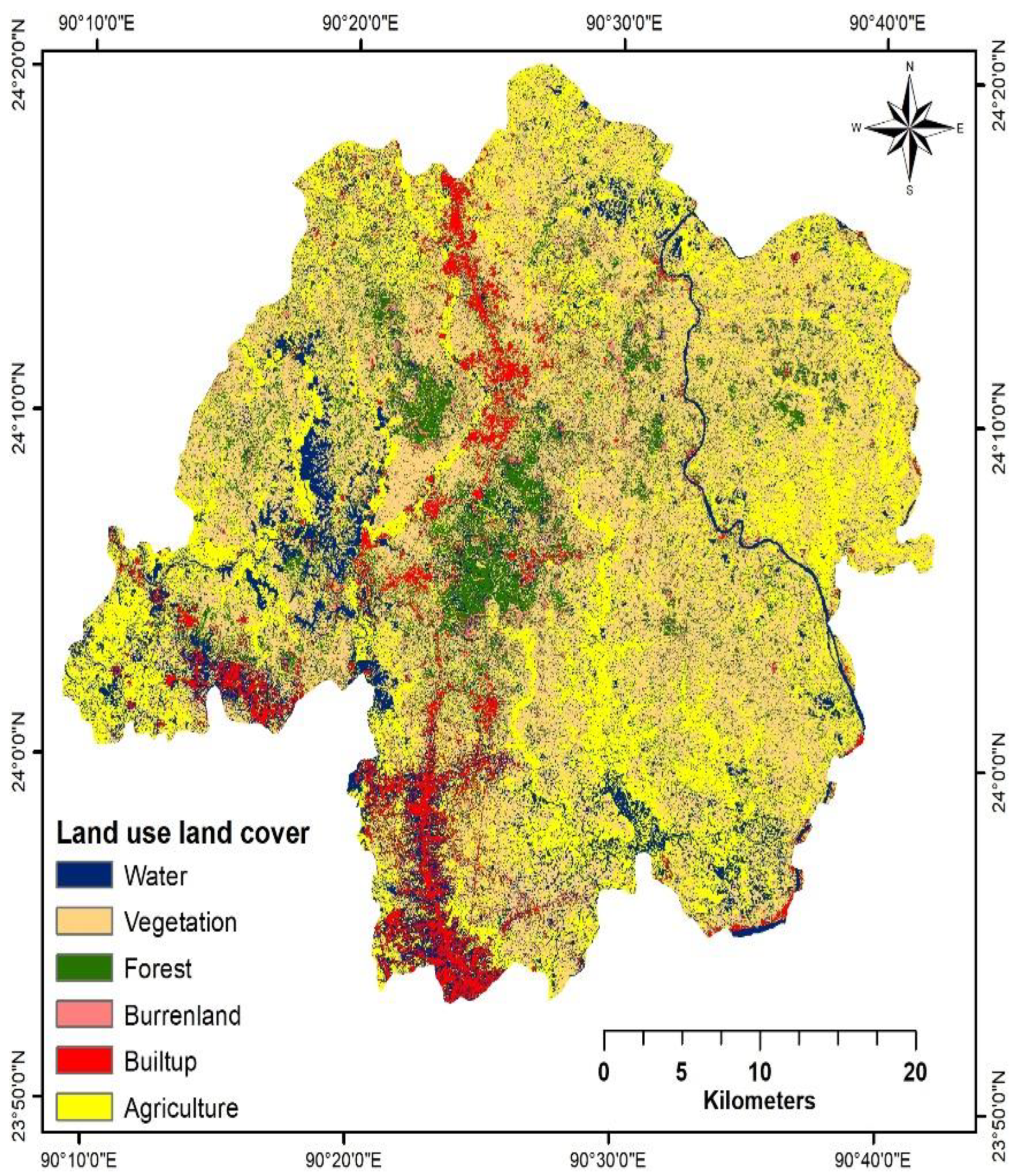
2.2.4. Land Use Land Cover (LULC)
2.2.5. Geology
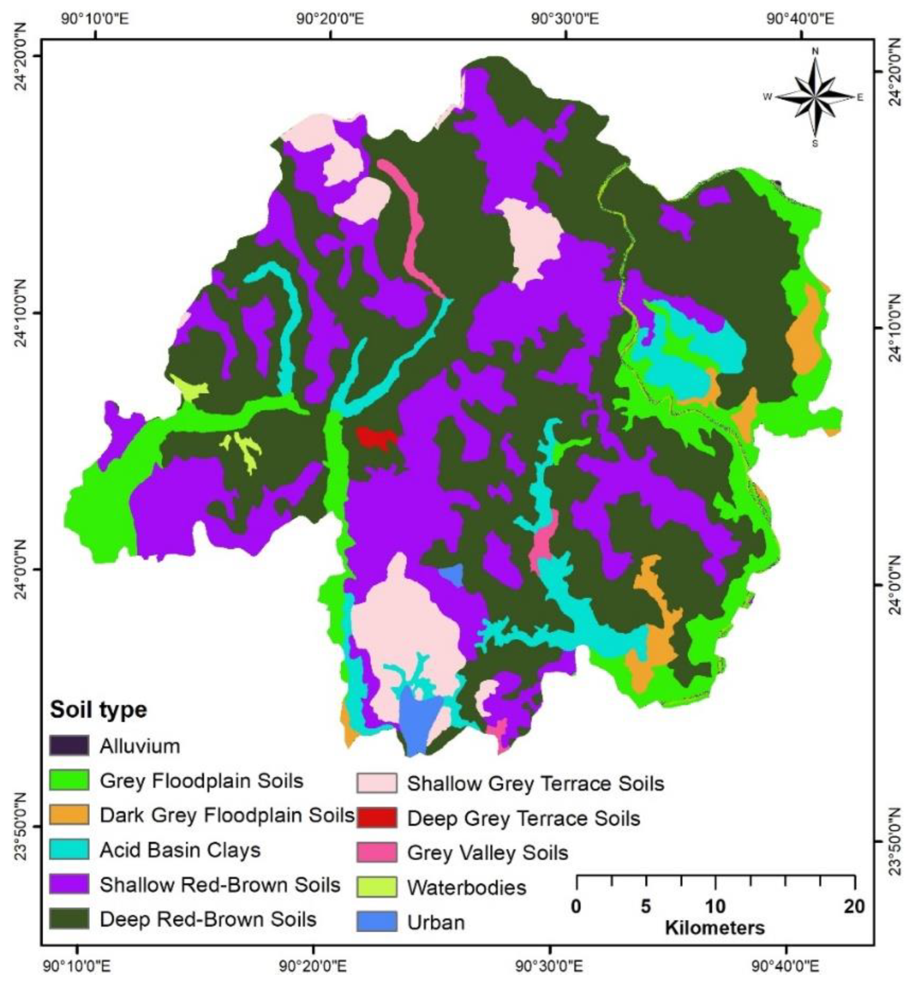
2.2.6. Soil Type
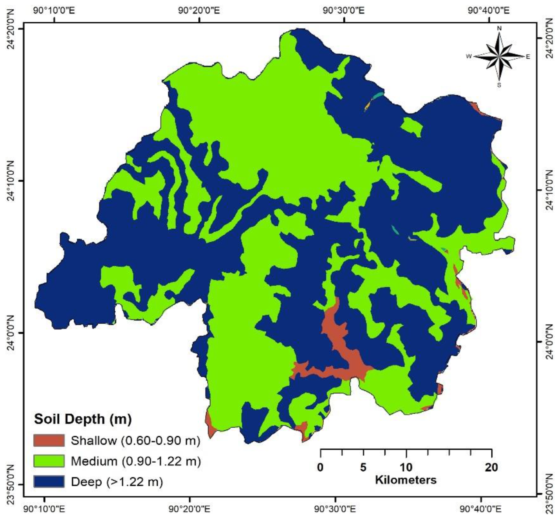
2.2.7. Soil Depth
2.2.8. Rainfall
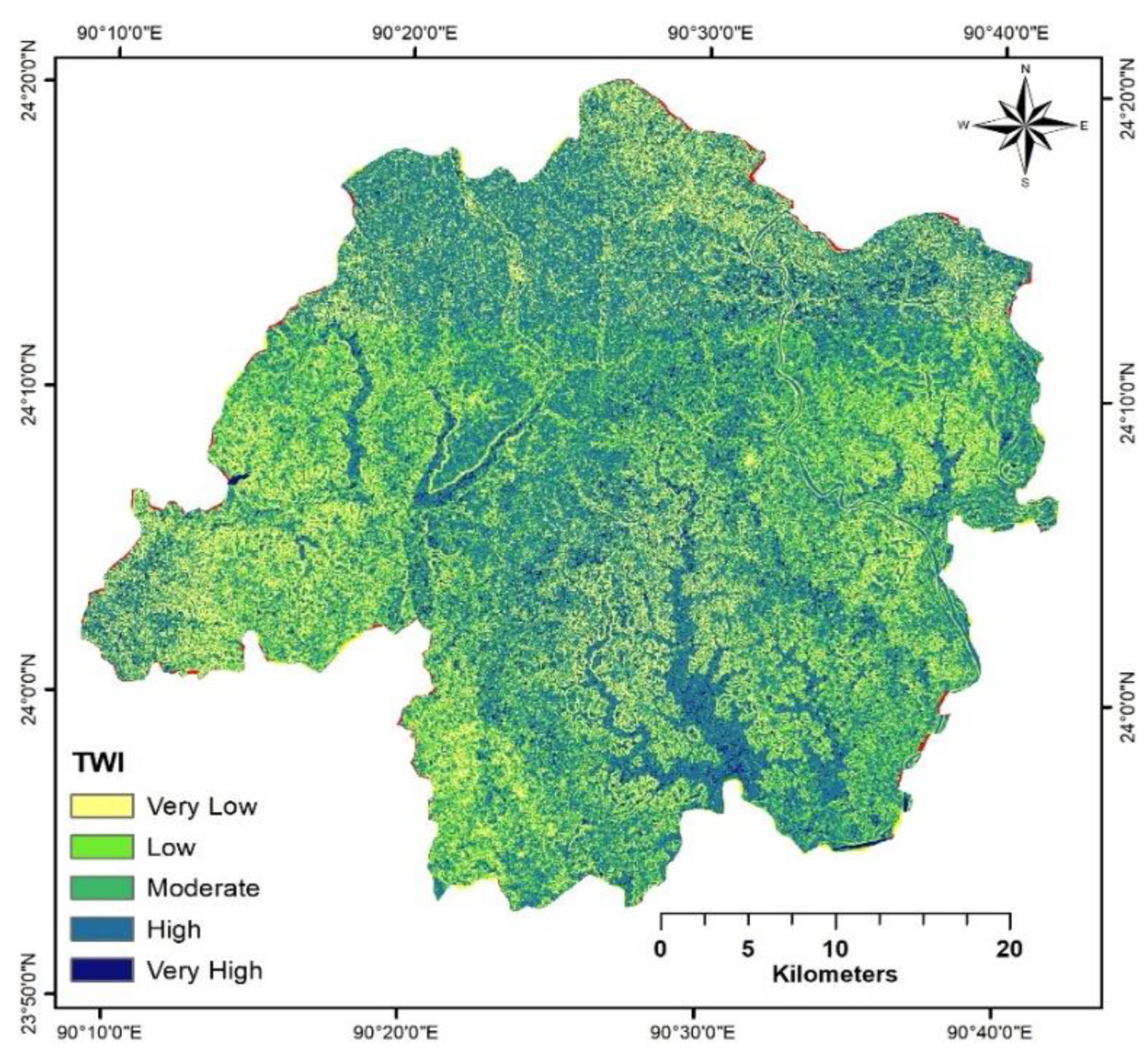
2.2.9. Topographic Wetness Index (TWI)
2.2.10. The Plan and Profile Curvature
2.3. Analytical Hierarchy Process (AHP) Model
2.4. Delineation of Groundwater Potential Zone (GWPZ)
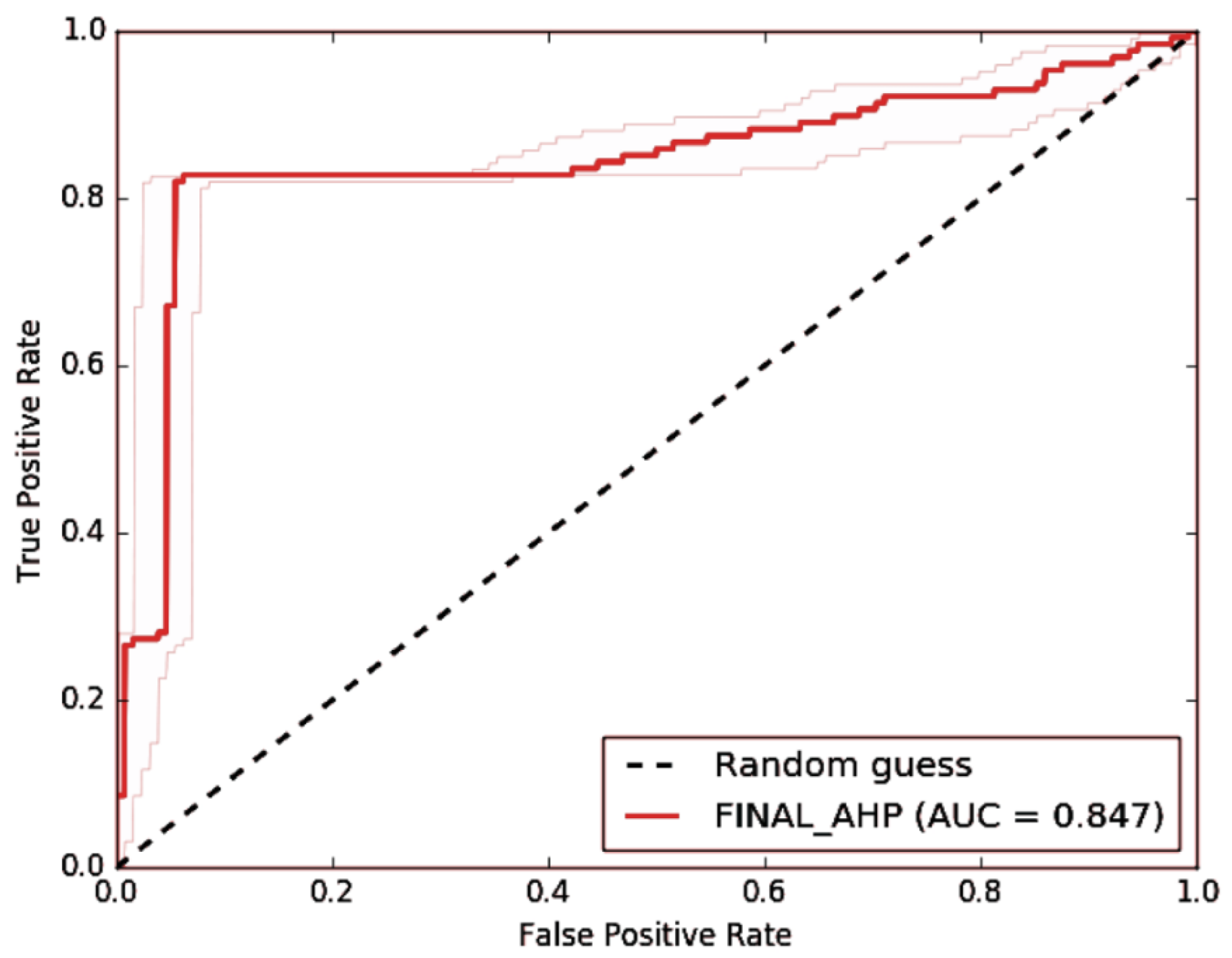
2.5. Validation of Groundwater Potential Zone
3. Results
3.1. Assessment of Factors Governing Groundwater Potential Zone
3.1.1. Geology
3.1.2. Land Use Land Cover
3.1.3. Slope
3.1.4. Lineament Density
3.1.5. Drainage Density
3.1.6. Rainfall
3.1.7. Soil Type
3.1.8. Soil Depth
3.1.9. Topographic Wetness Index
3.1.10. Plan and Profile Curvature
3.2. Groundwater Potential Map
3.3. Validation of the Groundwater Potential Zone
4. Discussion
5. Conclusions
Author Contributions
Funding
Institutional Review Board Statement
Informed Consent Statement
Data Availability Statement
Conflicts of Interest
References
- Shekhar, S.; Pandey, A.C. Delineation of groundwater potential zone in hard rock terrain of India using remote sensing, geographical information system (GIS) and analytic hierarchy process (AHP) techniques. Geocarto Int. 2014, 30, 402–421. [Google Scholar] [CrossRef]
- Naghibi, S.A.; Moghaddam, D.D.; Kalantar, B.; Pradhan, B.; Kisi, O. A comparative assessment of GIS-based data mining models and a novel ensemble model in groundwater well potential mapping. J. Hydrol. 2017, 548, 471–483. [Google Scholar] [CrossRef]
- Pande, C.B.; Moharir, K.N.; Panneerselvam, B.; Singh, S.K.; Elbeltagi, A.; Pham, Q.B.; Varade, A.M.; Rajesh, J. Delineation of groundwater potential zones for sustainable development and planning using analytical hierarchy process (AHP), and MIF techniques. Appl. Water Sci. 2021, 11, 186. [Google Scholar] [CrossRef]
- Haq, K.A. Water Management in Dhaka. Int. J. Water Resour. Dev. 2006, 22, 291–311. [Google Scholar] [CrossRef]
- Qureshi, A.; Ahmed, Z.; Krupnik, T. Groundwater Management in Bangladesh: An Analysis of Problems and Opportunities; Cereal Systems Inititave for South Asia Mechanization and Irrigation Project (CSISA-MI) Project; Research Report No. 2; CIMMYT: Dhaka, Bangladesh, 2014. [Google Scholar]
- Zahid, A.; Reaz, S.; Ahmed, U. Groundwater Resources Development in Bangladesh: Contribution to Irrigation for Food Security and Constraints to Sustainability. Groundw. Gov. Asia Ser. 2006, 1, 27–46. [Google Scholar]
- Jakob, M.C.; Jakob, D.M. Of the Revised Final Draft Report on Consolidation and Analysis of Information on Water Resources Management in Bangladesh. 2015. Available online: www.pwc.com/in (accessed on 28 December 2021).
- Jasrotia, A.S.; Kumar, A.; Singh, R. Integrated remote sensing and GIS approach for delineation of groundwater potential zones using aquifer parameters in Devak and Rui watershed of Jammu and Kashmir, India. Arab. J. Geosci. 2016, 9, 304. [Google Scholar] [CrossRef]
- Bhuiyan, C.; Singh, R.P.; Flügel, W.A. Modelling of ground water recharge-potential in the hard-rock Aravalli terrain, India: A GIS approach. Environ. Earth Sci. 2009, 59, 929–938. [Google Scholar] [CrossRef]
- Mcbean, E.; Gharabaghi, B. Groundwater in Bangladesh: Implications in a Climate-Changing World. Water Res. Manag. 2011, 1, 3–8. [Google Scholar]
- Shamsudduha, M.; Chandler, R.E.; Taylor, R.G.; Ahmed, K.M. Recent trends in groundwater levels in a highly seasonal hydrological system: The Ganges-Brahmaputra-Meghna Delta. Hydrol. Earth Syst. Sci. 2009, 13, 2373–2385. [Google Scholar] [CrossRef] [Green Version]
- Razandi, Y.; Pourghasemi, H.R.; Neisani, N.S.; Rahmati, O. Application of analytical hierarchy process, frequency ratio, and certainty factor models for groundwater potential mapping using GIS. Earth Sci. Inform. 2015, 8, 867–883. [Google Scholar] [CrossRef]
- Murmu, P.; Kumar, M.; Lal, D.; Sonker, I.; Singh, S.K. Delineation of groundwater potential zones using geospatial techniques and analytical hierarchy process in Dumka district, Jharkhand, India. Groundw. Sustain. Dev. 2019, 9, 100239. [Google Scholar] [CrossRef]
- Oh, H.-J.; Pradhan, B. Application of a neuro-fuzzy model to landslide-susceptibility mapping for shallow landslides in a tropical hilly area. Comput. Geosci. 2011, 37, 1264–1276. [Google Scholar] [CrossRef]
- Arkoprovo, B.; Adarsa, J.; Animesh, M. Application of Remote Sensing, GIS and MIF technique for Elucidation of Groundwater Potential Zones from a part of Orissa coastal tract. East. India 2013, 2, 42–49. [Google Scholar]
- Singh, S.K.; Singh, C.K.; Mukherjee, S. Impact of land-use and land-cover change on groundwater quality in the Lower Shiwalik hills: A remote sensing and GIS based approach. Open Geosci. 2010, 2, 124–131. [Google Scholar] [CrossRef]
- Adiat, K.; Nawawi, M.; Abdullah, K. Assessing the accuracy of GIS-based elementary multi criteria decision analysis as a spatial prediction tool—A case of predicting potential zones of sustainable groundwater resources. J. Hydrol. 2012, 440–441, 75–89. [Google Scholar] [CrossRef]
- Nampak, H.; Pradhan, B.; Manap, M.A. Application of GIS based data driven evidential belief function model to predict groundwater potential zonation. J. Hydrol. 2014, 513, 283–300. [Google Scholar] [CrossRef]
- Adeyeye, O.; Ikpokonte, E.; Arabi, S. GIS-based groundwater potential mapping within Dengi area, North Central Nigeria. Egypt. J. Remote Sens. Space Sci. 2018, 22, 175–181. [Google Scholar] [CrossRef]
- Patra, S.; Mishra, P.; Mahapatra, S.C. Delineation of groundwater potential zone for sustainable development: A case study from Ganga Alluvial Plain covering Hooghly district of India using remote sensing, geographic information system and analytic hierarchy process. J. Clean. Prod. 2018, 172, 2485–2502. [Google Scholar] [CrossRef]
- Andualem, T.G.; Demeke, G.G. Groundwater potential assessment using GIS and remote sensing: A case study of Guna tana landscape, upper blue Nile Basin, Ethiopia. J. Hydrol. Reg. Stud. 2019, 24, 100610. [Google Scholar] [CrossRef]
- Kaur, L.; Rishi, M.S.; Singh, G.; Thakur, S.N. Groundwater potential assessment of an alluvial aquifer in Yamuna sub-basin (Panipat region) using remote sensing and GIS techniques in conjunction with analytical hierarchy process (AHP) and catastrophe theory (CT). Ecol. Indic. 2019, 110, 105850. [Google Scholar] [CrossRef]
- Nithya, C.N.; Srinivas, Y.; Magesh, N.; Kaliraj, S. Assessment of groundwater potential zones in Chittar basin, Southern India using GIS based AHP technique. Remote Sens. Appl. Soc. Environ. 2019, 15, 100248. [Google Scholar] [CrossRef]
- Arulbalaji, P.; Padmalal, D.; Sreelash, K. GIS and AHP Techniques Based Delineation of Groundwater Potential Zones: A case study from Southern Western Ghats, India. Sci. Rep. 2019, 9, 2082. [Google Scholar] [CrossRef] [PubMed]
- Benjmel, K.; Amraoui, F.; Boutaleb, S.; Ouchchen, M.; Tahiri, A.; Touab, A. Mapping of Groundwater Potential Zones in Techniques, and Multicriteria Data Analysis. Water 2020, 12, 471. [Google Scholar] [CrossRef] [Green Version]
- Ahmadi, H.; Kaya, O.A.; Babadagi, E.; Savas, T.; Pekkan, E.H.; Ahmadi, O.A.; Kaya, E.; Babadagi, T.S.; Pekkan, E. GIS-Based Groundwater Potentiality Mapping Using AHP and FR Models in Central Antalya, Turkey. Environ. Sci. Proc. 2020, 5, 11. [Google Scholar] [CrossRef]
- Ozdemir, A. GIS-based groundwater spring potential mapping in the Sultan Mountains (Konya, Turkey) using frequency ratio, weights of evidence and logistic regression methods and their comparison. J. Hydrol. 2011, 411, 290–308. [Google Scholar] [CrossRef]
- Pourghasemi, H.R.; Beheshtirad, M. Assessment of a data-driven evidential belief function model and GIS for groundwater potential mapping in the Koohrang Watershed, Iran. Geocarto Int. 2014, 30, 662–685. [Google Scholar] [CrossRef]
- Lee, S.; Lee, C.-W. Application of Decision-Tree Model to Groundwater Productivity-Potential Mapping. Sustainability 2015, 7, 13416–13432. [Google Scholar] [CrossRef] [Green Version]
- Duan, H.; Deng, Z.; Deng, F.; Wang, D. Assessment of Groundwater Potential Based on Multicriteria Decision Making Model and Decision Tree Algorithms. Math. Probl. Eng. 2016, 2016, 2064575. [Google Scholar] [CrossRef] [Green Version]
- Raju, R.S.; Raju, G.S.; Rajasekhar, M.R.; Siddi Raju, G.; Sudarsana, R.; Rajasekhar, M. Identification of groundwater potential zones in Mandavi River basin, Andhra Pradesh, India using remote sensing, GIS and MIF techniques. HydroResearch 2019, 2, 1–11. [Google Scholar] [CrossRef]
- Thapa, R.; Gupta, S.; Guin, S.; Kaur, H. Assessment of groundwater potential zones using multi-influencing factor (MIF) and GIS: A case study from Birbhum district, West Bengal. Appl. Water Sci. 2017, 7, 4117–4131. [Google Scholar] [CrossRef]
- Abijith, D.; Saravanan, S.; Singh, L.; Jennifer, J.J.; Saranya, T.; Parthasarathy, K. GIS-based multi-criteria analysis for identification of potential groundwater recharge zones—A case study from Ponnaniyaru watershed, Tamil Nadu, India. J. Hydro-Environ. Res. 2020, 3, 1–14. [Google Scholar] [CrossRef]
- Mallick, J.; Khan, R.A.; Ahmed, M.; Alqadhi, S.D.; Alsubih, M.; Falqi, I.; Hasan, M.A. Modeling Groundwater Potential Zone in a Semi-Arid Region of Aseer Using Fuzzy-AHP and Geoinformation Techniques. Water 2019, 11, 2656. [Google Scholar] [CrossRef] [Green Version]
- Ankana; Dhanaraj, G. Study of selected influential criteria on groundwater potential storage using geospatial technology and multi-criteria decision analysis (MCDA) approach: A case study. Egypt. J. Remote Sens. Space Sci. 2021, 24, 649–658. [Google Scholar] [CrossRef]
- Srivastava, S.K. Delineation of Groundwater Potential Zone through Geospatial Technique, Multi-Criteria Decision Analysis, and Analytical Hierarchy Process. Res. Sq. 2021, 1–25. [Google Scholar] [CrossRef]
- Jhariya, D.C.; Khan, R.; Mondal, K.C.; Kumar, T.; Singh, V.K. Assessment of groundwater potential zone using GIS-based multi-influencing factor (MIF), multi-criteria decision analysis (MCDA) and electrical resistivity survey techniques in Raipur city, Chhattisgarh, India. J. Water Supply Res. Technol. 2021, 70, 375–400. [Google Scholar] [CrossRef]
- Anteneh, Z.L. Appraising groundwater potential zones using geospatial and multi-criteria decision analysis (MCDA) techniques in Andasa-Tul watershed, Upper Blue Nile basin, Ethiopia. Environ. Earth Sci. 2022, 81, 1–20. [Google Scholar] [CrossRef]
- Habibi, S.M.; Ono, H.; Shukla, A. Geographical Information System (GIS) Based Multi-Criteria Decision Analysis for Categorization of the Villages: In the Case of Kabul New City Villages. Urban Sci. 2021, 5, 65. [Google Scholar] [CrossRef]
- Babu, A.H.; Islam, R.; Farzana, F.; Uddin, M.J.; Islam, S. Application of GIS and Remote Sensing for Identification of Groundwater Potential Zone in the Hilly Terrain of Bangladesh. Grassroots J. Nat. Resour. 2020, 3, 16–27. [Google Scholar] [CrossRef]
- Ferozur, R.M.; Jahan, C.S.; Arefin, R.; Mazumder, Q.H. Groundwater potentiality study in drought prone barind tract, NW Bangladesh using remote sensing and GIS. Groundw. Sustain. Dev. 2018, 8, 205–215. [Google Scholar] [CrossRef]
- Hossain, I.; Bari, N.; Matin, I. Groundwater Zoning for the North-West Region of Bangladesh. Hydrology 2020, 8, 52. [Google Scholar] [CrossRef]
- Jahan, C.S.; Rahaman, F.; Arefin, R.; Ali, S.; Mazumder, Q.H. Delineation of groundwater potential zones of Atrai–Sib river basin in north-west Bangladesh using remote sensing and GIS techniques. Sustain. Water Resour. Manag. 2018, 5, 689–702. [Google Scholar] [CrossRef]
- Nowreen, S.; Newton, I.H.; Zzaman, R.U.; Islam, A.K.M.S.; Islam, G.M.T.; Alam, S. Development of potential map for groundwater abstraction in the northwest region of Bangladesh using RS-GIS-based weighted overlay analysis and water-table-fluctuation technique. Environ. Monit. Assess. 2021, 193, 24. [Google Scholar] [CrossRef] [PubMed]
- Shahinuzzaman, M.; Khan, M.N.U.; Islam, K.; Islam, Z. Identification of Potential Groundwater Bearing Zones by Hydrostratigrafic Analysis in the Eastern Part of Kushtia District. GUB J. Sci. Eng. 2021, 7, 36–41. [Google Scholar] [CrossRef]
- Sresto, M.A.; Siddika, S.; Haque, N.; Saroar, M. Application of fuzzy analytic hierarchy process and geospatial technology to identify groundwater potential zones in north-west region of Bangladesh. Environ. Chall. 2021, 5, 100214. [Google Scholar] [CrossRef]
- BBS. District Statistics of Gazipur. 2013. Available online: http://203.112.218.65:8008/WebTestApplication/userfiles/Image/DistrictStatistics/Gazipur.pdf (accessed on 30 July 2021).
- Mahmood, S.A. Beyond Dhaka and Gazipur: The Future of Industry; Dhaka Tribune: Dhaka, Bangladesh, 2021. [Google Scholar]
- Geological Survey (U.S.). Earth Explorer. 2000. Available online: https://earthexplorer.usgs.gov (accessed on 20 August 2021).
- Batelaan, O.; De Smedt, F. WetSpass: A Flexible, GIS Based, Distributed Recharge Methodology for Regional Groundwater Modelling; IAHS Publications: Wallingford, UK, 2001; pp. 11–18. [Google Scholar]
- Chaudhry, M.A.; Kumar, A.K.; Alam, K. Mapping of groundwater potential zones using the fuzzy analytic hierarchy process and geospatial technique. Geocarto Int. 2021, 36, 2323–2344. [Google Scholar] [CrossRef]
- Yeh, C.-H.; Cheng, H.-F.; Lin, Y.-S.; Lee, H.-I. Mapping groundwater recharge potential zone using a GIS approach in Hualian River, Taiwan. Sustain. Environ. Res. 2016, 26, 33–43. [Google Scholar] [CrossRef] [Green Version]
- Langbein, W.B.; Iseri, K.T. General Introduction End Hydrologic Definitions, Manual of Hydrology: Part 1. General Surface-Water Techniques. Geol. Surv. Water-Supply Pap. 1960, 1541-A, 33. [Google Scholar]
- Ganapuram, S.; Kumar, G.V.; Krishna, I.M.; Kahya, E.; Demirel, M.C. Mapping of groundwater potential zones in the Musi basin using remote sensing data and GIS. Adv. Eng. Softw. 2009, 40, 506–518. [Google Scholar] [CrossRef]
- Senthil Kumar, K.; Shankar, G.R. Assessment of groundwater potential zones using GIS technique. J. Indian Soc. Remote Sens. 2016, 37, 69–77. [Google Scholar] [CrossRef]
- Clark, C.; Wilson, C.D. Spatial analysis of lineaments. Comput. Geosci. 1994, 20, 1237–1258. [Google Scholar] [CrossRef]
- Ghodratabadi, S.; Feizi, F. Identification of groundwater potential zones in Moalleman, Iran by remote sensing and index overlay technique in GIS. Iran. J. Earth Sci. 2015, 7, 142–152. [Google Scholar]
- Nag, S.K.; Kundu, A. Application of remote sensing, GIS and MCA techniques for delineating groundwater prospect zones in Kashipur block, Purulia district, West Bengal. Appl. Water Sci. 2018, 8, 38. [Google Scholar] [CrossRef] [Green Version]
- Alobeid, A.; Aldosari, A.; Alrajhi, M.; Khan, M. Alternative approach for Recognition of Potential Ground Water Zones Using GIS and Remote Sensing_final_30-7-2015. Int. J. Appl. Remote Sens. GIS 2015, 2, 10–25. [Google Scholar]
- Das, B.; Pal, S.C.; Malik, S.; Chakrabortty, R. Modeling groundwater potential zones of Puruliya district, West Bengal, India using remote sensing and GIS techniques. Geol. Ecol. Landsc. 2018, 3, 223–237. [Google Scholar] [CrossRef] [Green Version]
- Yimer, F.; Messing, I.; Ledin, S.; Abdelkadir, A. Effects of different land use types on infiltration capacity in a catchment in the highlands of Ethiopia. Soil Use Manag. 2008, 24, 344–349. [Google Scholar] [CrossRef]
- Gorelick, N.; Hancher, M.; Dixon, M.; Ilyushchenko, S.; Thau, D.; Moore, R. Google Earth Engine: Planetary-scale geospatial analysis for everyone. Remote Sens. Environ. 2017, 202, 18–27. [Google Scholar] [CrossRef]
- Halder, S.; Roy, M.B.; Roy, P.K. Fuzzy logic algorithm based analytic hierarchy process for delineation of groundwater potential zones in complex topography. Arab. J. Geosci. 2020, 13, 574. [Google Scholar] [CrossRef]
- Kim, S.Y.; Lee, H. Effect of quality characteristics on brown rice produced from paddy rice with different moisture contents. J. Korean Soc. Appl. Biol. Chem. 2013, 56, 289–293. [Google Scholar] [CrossRef]
- BARC. Land Resources Appraisal of Bangladesh for Agricultural Development. 1988. Available online: http://www.barc.gov.bd (accessed on 30 November 2021).
- Patton, N.R.; Lohse, K.A.; Godsey, S.E.; Crosby, B.T.; Seyfried, M.S. Predicting soil thickness on soil mantled hillslopes. Nat. Commun. 2018, 9, 3329. [Google Scholar] [CrossRef]
- Hewlett, A.R.; Hibbert, J.D. Factors affecting the response of small watersheds to precipitation in humid areas. For. Hydrol. 1967, 1, 275–290. [Google Scholar]
- Nicotina, A.; Tarboton, L.; Tesfa, D.G.; Rinaldo, T.K. Hydrologic controls on equilibrium soil depths. Water Resour. Res. 2011, 47, 4. [Google Scholar] [CrossRef] [Green Version]
- Evaristo, J.; Jasechko, S.; McDonnell, J.J. Global separation of plant transpiration from groundwater and streamflow. Nature 2015, 525, 91–94. [Google Scholar] [CrossRef] [PubMed]
- Islam, A.; Cartwright, N. Evaluation of climate reanalysis and space-borne precipitation products over Bangladesh. Hydrol. Sci. J. 2020, 65, 1112–1128. [Google Scholar] [CrossRef]
- Kamruzzaman, M.; Shahid, S.; Roy, D.K.; Islam, A.R.M.T.; Hwang, S.; Cho, J.; Zaman, A.U.; Sultana, T.; Rashid, T.; Akter, F. Assessment of CMIP6 global climate models in reconstructing rainfall climatology of Bangladesh. Int. J. Clim. 2021. [Google Scholar] [CrossRef]
- Copernicus Climate Change Service (C3S). ERA5: Fifth Generation of ECMWF Atmospheric Reanalyses of the Global Climate. Copernicus Climate Change Service Climate Data Store (CDS). 2017. Available online: https://www.ecmwf.int/en/forecasts/datasets/reanalysis-datasets/era5 (accessed on 20 January 2021).
- Achilleos, G. The Inverse Distance Weighted interpolation method and error propagation mechanism—Creating a DEM from an analogue topographical map. J. Spat. Sci. 2011, 56, 283–304. [Google Scholar] [CrossRef]
- Arheimer, J.; Dahne, B.; Lindstrom, J.; Marklund, G.; Strömqvist, L. Multi-Variable Evaluation of an Integrated Model System Covering Sweden (S-HYPE); IAHS-AISH Publications: Wallingford, UK, 1979; Volume 345, pp. 145–150. [Google Scholar]
- Sørensen, R.; Zinko, U.; Seibert, J. On the calculation of the topographic wetness index: Evaluation of different methods based on field observations. Hydrol. Earth Syst. Sci. 2006, 10, 101–112. [Google Scholar] [CrossRef] [Green Version]
- Fazal, S.A.; Bhuiyan, M.A.H.M.; Chowdhury, M.A.I.; Kabir, M. Effects of Industrial Agglomeration on Land-Use Patterns and Surface Water Effects of Industrial Agglomeration on Land-Use Patterns and Surface Water Quality in Konabari, BSCIC area at Gazipur, Bangladesh. Int. Res. J. Environ. Sci. 2016, 4, 42–49. [Google Scholar]
- Al-Abadi, A.M.; Al-Temmeme, A.A.; Al-Ghanimy, M.A. A GIS-based combining of frequency ratio and index of entropy approaches for mapping groundwater availability zones at Badra–Al Al-Gharbi–Teeb areas, Iraq. Sustain. Water Resour. Manag. 2016, 2, 265–283. [Google Scholar] [CrossRef] [Green Version]
- Su, Z. Remote sensing of land use and vegetation for mesoscale hydrological studies. Int. J. Remote Sens. 2000, 21, 213–233. [Google Scholar] [CrossRef]
- Saaty, T.L. Decision Making for Leaders: The Analytic Hierarchy Process for Decisions in a Complex World; RWS Publications: Cologne, Germany, 1990. [Google Scholar]
- Muralitharan, J.; Palanivel, K. Groundwater targeting using remote sensing, geographical information system and analytical hierarchy process method in hard rock aquifer system, Karur district, Tamil Nadu, India. Earth Sci. Inform. 2015, 8, 827–842. [Google Scholar] [CrossRef]
- Saaty, R.W. The analytic hierarchy process—What it is and how it is used. Math. Model. 1987, 9, 161–176. [Google Scholar] [CrossRef] [Green Version]
- Saaty, T. A scaling method for priorities in hierarchical structures. J. Math. Psychol. 1977, 15, 234–281. [Google Scholar] [CrossRef]
- Jensen, J.R. Introductory Digital Image Processing: A Remote Sensing Perspective, 2nd ed.; Prentice Hall, Inc.: Upper Saddle River, NJ, USA, 1996. [Google Scholar]
- Rajasekhar, M.; Sudarsana Raju, G.; Siddi Raju, R. Assessment of groundwater potential zones in parts of the semi-arid region of Anantapur District, Andhra Pradesh, India using GIS and AHP approach. Model. Earth Syst. Environ. 2019, 5, 1303–1317. [Google Scholar] [CrossRef]
- Das, M.; Parveen, T.; Ghosh, D.; Alam, J. Assessing groundwater status and human perception in drought-prone areas: A case of Bankura-I and Bankura-II blocks, West Bengal (India). Environ. Earth Sci. 2021, 80, 636. [Google Scholar] [CrossRef]
- Asmael, N.M. A GIS Based Weight of Evidence for Prediction Urban Growth of Baghdad City by Using Remote Sensing Data. Al-Nahrain J. Eng. Sci. 2015, 18. Available online: https://www.iasj.net/iasj?func=fulltext&aId=106779 (accessed on 30 July 2021).
- Kamiński, M. The impact of quality of digital elevation models on the result of landslide susceptibility modeling using the method of weights of evidence. Geosciences 2020, 10, 488. [Google Scholar] [CrossRef]
- Silwal, C.B.; Pathak, D. Review on Practices and State of the Art Methods on Delineation of Ground Water Potential Using GIS and Remote Sensing. Bull. Dep. Geol. 2018, 7–20. [Google Scholar] [CrossRef] [Green Version]
- Hwang, C.L.; Chen, P.F.; Hwang, S.J. Fuzzy Multiple Attribute Decision Making: Methods and Applications; Springer: Berlin/Heidelberg, Germany, 1992. [Google Scholar]
- Zhang, Z.; Xu, Y. Efficiency evaluation of sustainable water management using the HF-TODIM method. Int. Trans. Oper. Res. 2019, 26, 747–764. [Google Scholar] [CrossRef]
- Rao, B.A.; Briz-Kishore, B.V. Methodology for locating potential aquifers in a typical semi-arid region in India using resistivity and hydrogeologic parameters. Geoexploration 1991, 27, 55–64. [Google Scholar]
- Waikar, M.L.; Nilawar, A.P. Identification of Groundwater Potential Zone using Remote Sensing and GIS Technique. Int. J. Innov. Res. Sci. Eng. Technol. 2014, 3, 12163–12174. [Google Scholar]
- Mandal, P.; Saha, J.; Bhattacharya, S.; Paul, S. Delineation of groundwater potential zones using the integration of geospatial and MIF techniques: A case study on Rarh region of West Bengal, India. Environ. Chall. 2021, 5, 100396. [Google Scholar] [CrossRef]
- Brammer, H.; Antoine, J.; Kassam, A.H.; Van Velthuizen, H.T. Land Resources Appraisal of Bangladesh for Agricultural Development. Report-2 (BGD/81/035). FAO of United Nations, Rome. 20, 1988. Available online: http://bfis.bforest.gov.bd/library/wp-content/uploads/2019/04/8099.pdf (accessed on 30 July 2021).
- Acharya, T.; Nag, S.K. Study of Groundwater Prospects of the Crystalline Rocks in Purulia District, West Bengal, India Using Remote Sensing Data. Earth Resour. 2013, 1, 54–59. [Google Scholar] [CrossRef]
- Ajibade, B.; Olajire, F.O.; Ajibade, O.O.; Fadugba, T.F.; Idowu, O.G.; Adelodun, T.E.; Pham, Q.B. Groundwater potential assessment as a preliminary step to solving water scarcity challenges in Ekpoma, Edo State, Nigeria. Acta Geophys. 2021, 69, 1367–1381. [Google Scholar] [CrossRef]
- Das, S.D.; Pardeshi, S. Integration of different influencing factors in GIS to delineate groundwater potential areas using IF and FR techniques: A study of Pravara basin, Maharashtra, India. Appl. Water Sci. 2018, 8, 1–16. [Google Scholar] [CrossRef] [Green Version]


| Upazila | Garments | Textile | Match Factory | Rice Mill | Steel and Engineering | Aluminum Factory | Jute Mill | Others |
|---|---|---|---|---|---|---|---|---|
| Gazipur Sadar | 822 | 73 | 2 | 227 | 27 | 9 | 0 | 203 |
| Kalikair | 51 | 35 | 0 | 45 | 2 | 1 | 2 | 17 |
| Kaligang | 0 | 0 | 0 | 62 | 0 | 0 | 1 | 4 |
| Kapasia | 0 | 0 | 0 | 14 | 0 | 0 | 0 | 3 |
| Sreepur | 25 | 19 | 0 | 42 | 0 | 2 | 0 | 85 |
| Total | 898 | 127 | 2 | 390 | 29 | 12 | 3 | 312 |
| Importance | Description |
|---|---|
| 1 | Equal importance |
| 2 | Equal to moderate importance |
| 3 | Moderate importance |
| 4 | Moderate to strong importance |
| 5 | Strong importance |
| 6 | Strong to very strong importance |
| 7 | Very strong importance |
| 8 | Very to extremely strong importance |
| 9 | Extreme importance |
| Factors | Geology | LULC | Lineament | Drainage | Slope | Rainfall | Soil | Soil Depth | TWI | Plan Cur. | Profile Cur. |
|---|---|---|---|---|---|---|---|---|---|---|---|
| Geology | 1.000 | 1.143 | 1.333 | 1.333 | 1.333 | 1.600 | 1.600 | 1.600 | 2.000 | 2.667 | 2.667 |
| LULC | 0.875 | 1.000 | 1.167 | 1.167 | 1.167 | 1.400 | 1.400 | 1.400 | 1.750 | 2.333 | 2.333 |
| Lineament Density | 0.750 | 0.857 | 1.000 | 1.000 | 1.000 | 1.200 | 1.200 | 1.200 | 1.500 | 2.000 | 2.000 |
| Drainage Density | 0.750 | 0.857 | 1.000 | 1.000 | 1.000 | 1.200 | 1.200 | 1.200 | 1.500 | 2.000 | 2.000 |
| Slope | 0.750 | 0.857 | 1.000 | 1.000 | 1.000 | 1.200 | 1.200 | 1.200 | 1.500 | 2.000 | 2.000 |
| Rainfall | 0.625 | 0.714 | 0.833 | 0.833 | 0.833 | 1.000 | 1.000 | 1.000 | 1.250 | 1.667 | 1.667 |
| Soil | 0.625 | 0.714 | 0.833 | 0.833 | 0.833 | 1.000 | 1.000 | 1.000 | 1.250 | 1.667 | 1.667 |
| Soil depth | 0.625 | 0.714 | 0.833 | 0.833 | 0.833 | 1.000 | 1.000 | 1.000 | 1.250 | 1.667 | 1.667 |
| TWI | 0.500 | 0.571 | 0.667 | 0.667 | 0.667 | 0.800 | 0.800 | 0.800 | 1.000 | 1.333 | 1.333 |
| Plan Curvature | 0.375 | 0.429 | 0.500 | 0.500 | 0.500 | 0.600 | 0.600 | 0.600 | 0.750 | 1.000 | 1.000 |
| Profile Curvature | 0.375 | 0.429 | 0.500 | 0.500 | 0.500 | 0.600 | 0.600 | 0.600 | 0.750 | 1.000 | 1.000 |
| Total | 7.250 | 8.286 | 9.667 | 9.667 | 9.667 | 11.600 | 11.600 | 11.600 | 14.500 | 19.333 | 19.333 |
| Factors | Geology | LULC | Lineament | Drainage | Slope | Rainfall | Soil | Soil Depth | TWI | Plan Cur. | Profile Cur. | Eigen Vector | AHP Weight (%) |
|---|---|---|---|---|---|---|---|---|---|---|---|---|---|
| Geology | 0.137 | 0.138 | 0.137 | 0.137 | 0.138 | 0.137 | 0.138 | 0.138 | 0.138 | 0.138 | 0.138 | 0.138 | 14 |
| LULC | 0.121 | 0.121 | 0.121 | 0.121 | 0.121 | 0.121 | 0.121 | 0.121 | 0.121 | 0.121 | 0.121 | 0.121 | 12 |
| Lineament | 0.103 | 0.103 | 0.103 | 0.103 | 0.103 | 0.103 | 0.103 | 0.103 | 0.103 | 0.103 | 0.103 | 0.103 | 10 |
| Drainage | 0.103 | 0.103 | 0.103 | 0.103 | 0.103 | 0.103 | 0.103 | 0.103 | 0.103 | 0.103 | 0.103 | 0.103 | 10 |
| Slope | 0.103 | 0.103 | 0.103 | 0.103 | 0.103 | 0.103 | 0.103 | 0.103 | 0.103 | 0.103 | 0.103 | 0.103 | 10 |
| Rainfall | 0.086 | 0.086 | 0.086 | 0.086 | 0.086 | 0.086 | 0.086 | 0.086 | 0.086 | 0.086 | 0.086 | 0.086 | 9 |
| Soil | 0.086 | 0.086 | 0.086 | 0.086 | 0.086 | 0.086 | 0.086 | 0.086 | 0.086 | 0.086 | 0.086 | 0.086 | 9 |
| Soil depth | 0.086 | 0.086 | 0.086 | 0.086 | 0.086 | 0.086 | 0.086 | 0.086 | 0.086 | 0.086 | 0.086 | 0.086 | 9 |
| TWI | 0.069 | 0.069 | 0.068 | 0.068 | 0.069 | 0.069 | 0.069 | 0.068 | 0.069 | 0.068 | 0.068 | 0.068 | 7 |
| Plan Cur. | 0.052 | 0.052 | 0.052 | 0.052 | 0.052 | 0.052 | 0.052 | 0.052 | 0.052 | 0.052 | 0.052 | 0.052 | 5 |
| Profile Cur. | 0.052 | 0.052 | 0.052 | 0.052 | 0.052 | 0.052 | 0.052 | 0.052 | 0.052 | 0.052 | 0.052 | 0.052 | 5 |
| Sum | 1.00 | 1.00 | 1.00 | 1.00 | 1.00 | 1.00 | 1.00 | 1.00 | 1.00 | 1.00 | 1.00 | 1.00 | 100 |
| n | 1 | 2 | 3 | 4 | 5 | 6 | 7 | 8 | 9 | 10 | 11 |
|---|---|---|---|---|---|---|---|---|---|---|---|
| RI | 0.00 | 0.00 | 0.52 | 0.89 | 1.11 | 1.12 | 1.35 | 1.40 | 1.45 | 1.49 | 1.52 |
| Factor | Sub-Classes | Assigned Rank | AHP | ||
|---|---|---|---|---|---|
| Weight | Rating | Total | |||
| Alluvial silt | 3 | 0.42 | |||
| Alluvial silt and clay | 4 | 0.56 | |||
| Geology | Lake | 5 | 0.14 | 0.70 | 2.94 |
| Marsh clay and peat | 4 | 0.56 | |||
| Modhupur clay residuum | 5 | 0.70 | |||
| Forest | 3 | 0.36 | |||
| Waterbody | 5 | 0.60 | |||
| Agriculture Land | 4 | 0.48 | |||
| LULC | Vegetation | 3 | 0.12 | 0.36 | 2.64 |
| Urban Area | 2 | 0.24 | |||
| Fellow Land | 3 | 0.36 | |||
| Settlement vegetation | 2 | 0.24 | |||
| Very low | 2 | 0.20 | |||
| Low | 3 | 0.30 | |||
| Lineament | Medium | 4 | 0.1 | 0.40 | 2.00 |
| High | 5 | 0.50 | |||
| Very high | 6 | 0.60 | |||
| Very low | 2 | 0.20 | |||
| Low | 3 | 0.30 | |||
| Rainfall | Medium | 4 | 0.1 | 0.40 | 2.00 |
| High | 5 | 0.50 | |||
| Very high | 6 | 0.60 | |||
| Shallow | 5 | 0.50 | |||
| Soil Depth | Medium | 4 | 0.1 | 0.40 | 1.20 |
| Deep | 3 | 0.30 | |||
| Very low | 6 | 0.54 | |||
| Low | 5 | 0.45 | |||
| Drainage Density | Medium | 4 | 0.09 | 0.36 | 1.80 |
| High | 3 | 0.27 | |||
| Very high | 2 | 0.18 | |||
| Noncalcareous Alluvium | 1 | 0.09 | |||
| Grey Floodplain Soils | 2 | 0.18 | |||
| Dark Grey Floodplain | 2 | 0.18 | |||
| Acid Basin Clays | 5 | 0.45 | |||
| Shallow Red-Brown Terrace Soils | 5 | 0.45 | |||
| Soil | Deep Red-Brown Terrace Soils | 5 | 0.09 | 0.45 | 3.33 |
| Shallow Grey Terrace Soils | 3 | 0.27 | |||
| Deep Grey Terrace Soils | 3 | 0.27 | |||
| Waterbodies | 5 | 0.45 | |||
| Urban | 2 | 0.18 | |||
| Grey Valley Soils | 4 | 0.36 | |||
| Very low | 6 | 0.54 | |||
| Low | 5 | 0.45 | |||
| Slope | Medium | 4 | 0.09 | 0.36 | 1.80 |
| High | 3 | 0.27 | |||
| Very high | 2 | 0.18 | |||
| Very low | 2 | 0.14 | |||
| Low | 3 | 0.21 | |||
| TWI | Medium | 4 | 0.07 | 0.28 | 1.40 |
| High | 5 | 0.35 | |||
| Very high | 6 | 0.42 | |||
| Very low | 2 | 0.10 | |||
| Low | 3 | 0.15 | |||
| Plane curvature | Medium | 4 | 0.05 | 0.20 | 1.00 |
| High | 5 | 0.25 | |||
| Very high | 6 | 0.30 | |||
| Very low | 2 | 0.10 | |||
| Low | 3 | 0.15 | |||
| Profile curvature | Medium | 4 | 0.05 | 0.20 | 1.00 |
| High | 5 | 0.25 | |||
| Very high | 6 | 0.30 | |||
| Potential Level | Total Area (km2) | Area (%) |
|---|---|---|
| Very Low | 0.028 | 0.002 |
| Low | 63.182 | 3.830 |
| Medium | 927.047 | 56.201 |
| High | 647.456 | 39.251 |
| Very High | 11.815 | 0.716 |
| total | 1649.528 | 100 |
| Sub District | Potential Level | TOPSIS Analysis | |||||
|---|---|---|---|---|---|---|---|
| Very Low | Low | Moderate | High | Very High | Performance Index | Rank | |
| Gazipur | 0.00 | 3.73 | 54.14 | 41.42 | 0.70 | 0.52 | 4 |
| Sreepur | 0.00 | 2.05 | 52.27 | 45.33 | 0.34 | 0.80 | 1 |
| Kapasia | 0.00 | 3.92 | 58.15 | 36.57 | 1.36 | 0.62 | 2 |
| Kaliganj | 0.00 | 8.95 | 68.76 | 21.94 | 0.35 | 0.39 | 5 |
| Kaliakoir | 0.00 | 3.22 | 54.16 | 41.82 | 0.80 | 0.61 | 3 |
| Upazila | Well ID | Lat | Lon | Water Table (m) | Actual | AHP Model | |
|---|---|---|---|---|---|---|---|
| Class | Remarks | ||||||
| Gazipur Sadar | GT3330001 | 23.93 | 90.42 | 7.98 | Very Good | High | Agreed |
| Gazipur Sadar | GT3330002 | 23.96 | 90.48 | 13.01 | Good | High | Agreed |
| Gazipur Sadar | GT3330020 | 23.9 | 90.39 | 24.00 | Poor | Moderate | Not Agreed |
| Kaliakair | GT3332003 | 24.11 | 90.3 | 10.62 | Good | High | Agreed |
| Kaliakair | GT3332004 | 24.21 | 90.32 | 8.23 | Good | Moderate | Agreed |
| Kaliakair | GT3332005 | 24.16 | 90.31 | 10.25 | Good | High | Agreed |
| Kaliakair | GT3332006 | 24.09 | 90.34 | 6.51 | Very Good | High | Agreed |
| Kaliakair | GT3332007 | 24.15 | 90.35 | 5.68 | Very Good | High | Agreed |
| Kaliakair | GT3332008 | 24.13 | 90.28 | 10.03 | Good | Moderate | Agreed |
| Kaliganj | GT3334009 | 23.96 | 90.54 | 4.44 | Very Good | Moderate | Not Agreed |
| Kaliganj | GT3334010 | 24.00 | 90.58 | 7.45 | Very Good | Moderate | Not Agreed |
| Kapasia | GT3336011 | 24.2 | 90.63 | 5.11 | Very Good | High | Agreed |
| Kapasia | GT3336012 | 24.16 | 90.67 | 4.73 | Very Good | High | Agreed |
| Kapasia | GT3336013 | 24.13 | 90.62 | 4.51 | Very Good | High | Agreed |
| Sreepur | GT3386014 | 24.22 | 90.48 | 5.96 | Very Good | High | Agreed |
| Sreepur | GT3386015 | 24.18 | 90.54 | 5.99 | Very Good | Moderate | Not Agreed |
| Sreepur | GT3386017 | 24.17 | 90.51 | 9.83 | Good | High | Agreed |
| Sreepur | GT3386018 | 24.27 | 90.53 | 7.78 | Good | High | Agreed |
| Sreepur | GT3386019 | 24.28 | 90.35 | 9.52 | Good | High | Agreed |
| Kaliganj | GT6768008 | 24.28 | 90.49 | 7.27 | Very Good | High | Agreed |
Publisher’s Note: MDPI stays neutral with regard to jurisdictional claims in published maps and institutional affiliations. |
© 2022 by the authors. Licensee MDPI, Basel, Switzerland. This article is an open access article distributed under the terms and conditions of the Creative Commons Attribution (CC BY) license (https://creativecommons.org/licenses/by/4.0/).
Share and Cite
Rahman, M.M.; AlThobiani, F.; Shahid, S.; Virdis, S.G.P.; Kamruzzaman, M.; Rahaman, H.; Momin, M.A.; Hossain, M.B.; Ghandourah, E.I. GIS and Remote Sensing-Based Multi-Criteria Analysis for Delineation of Groundwater Potential Zones: A Case Study for Industrial Zones in Bangladesh. Sustainability 2022, 14, 6667. https://doi.org/10.3390/su14116667
Rahman MM, AlThobiani F, Shahid S, Virdis SGP, Kamruzzaman M, Rahaman H, Momin MA, Hossain MB, Ghandourah EI. GIS and Remote Sensing-Based Multi-Criteria Analysis for Delineation of Groundwater Potential Zones: A Case Study for Industrial Zones in Bangladesh. Sustainability. 2022; 14(11):6667. https://doi.org/10.3390/su14116667
Chicago/Turabian StyleRahman, Md. Mizanur, Faisal AlThobiani, Shamsuddin Shahid, Salvatore Gonario Pasquale Virdis, Mohammad Kamruzzaman, Hafijur Rahaman, Md. Abdul Momin, Md. Belal Hossain, and Emad Ismat Ghandourah. 2022. "GIS and Remote Sensing-Based Multi-Criteria Analysis for Delineation of Groundwater Potential Zones: A Case Study for Industrial Zones in Bangladesh" Sustainability 14, no. 11: 6667. https://doi.org/10.3390/su14116667
APA StyleRahman, M. M., AlThobiani, F., Shahid, S., Virdis, S. G. P., Kamruzzaman, M., Rahaman, H., Momin, M. A., Hossain, M. B., & Ghandourah, E. I. (2022). GIS and Remote Sensing-Based Multi-Criteria Analysis for Delineation of Groundwater Potential Zones: A Case Study for Industrial Zones in Bangladesh. Sustainability, 14(11), 6667. https://doi.org/10.3390/su14116667