Article

The Impact of the Dynamics of Agglomeration Externalities on Air Pollution: Evidence from Urban Panel Data in China

1
School of Public Administration, Hohai University, Nanjing 211100, China
2
School of Economics and Management, Fuzhou University, Fuzhou 350116, China
*
Authors to whom correspondence should be addressed.
Sustainability 2022, 14(1), 580; https://doi.org/10.3390/su14010580
Submission received: 8 October 2021 / Revised: 5 December 2021 / Accepted: 28 December 2021 / Published: 5 January 2022

Abstract

:
Air pollution in China has become a matter of increasing public concern. In this paper, we attempted to build a theoretical model to explore the impact of the dynamics of agglomeration externalities on haze pollution in urban China, where agglomeration is differentiated by regional specialization and geographical concentration. Based on China’s panel data for 289 cities during the period of 1998–2018, the empirical result shows that the relationship between industrial agglomeration and urban haze pollution is not simply linear or of an inversed U-type but turns out to be dynamically N-shaped. To be specific, the increase in local haze pollution can be explained by agglomeration externalities in the beginning stage, whereas the reducing effect only occurs during the mature stage. The heterogeneity test indicated that the effect of the type of agglomeration on haze pollution seems to be mixed in different groups of cities, but is still consistent with the hypothesis of the dynamic change of agglomeration externalities. The results are found to be quite robust and consistent after replacing variables and using other regression methods. This paper provides answers to the question of how to coordinate the relationship between developing industry parks and air pollution in terms of the life cycle of agglomeration as well as the types of city.

1. Introduction

Since the beginning of the reform and opening-up policy in 1978, the Chinese economy has experienced a transformation from a centrally planned market to a fully fledged market, which led to the phenomenon of more enterprises becoming concentrated in some areas, such as the Yangtze River Delta and Pearl River Delta. In the process of industrialization and urbanization, China’s local governments—whether in eastern, central or western regions—have adopted a strategy of industry clustering to promote regional economic growth [1,2,3]. Agglomeration serves as a powerful engine for productivity growth and economic development, but it also causes numerous pollutants such as water pollution, soil pollution, and air pollution [4,5]. According to the statistics from the Ministry of Ecology and Environment [6], 180 cities of the 337 prefecture-level cities in China cannot meet national air quality standards, indicating that people in 180 cities are exposed to air pollution. Among the numerous air pollutants, fine particular matter (PM2.5) pollution is particularly prominent. It is clear that the concentration of PM2.5 can not only increase the formation of fog and haze weather, but also increase the risk of morbidity and mortality for residents [7,8,9,10]. In this context, the question of how to reduce PM2.5 pollution has become of increasing public concern as industrialization and urbanization develop rapidly in China, where the economy is experiencing the transition from high speed growth to high quality development.
There are two classic hypotheses on environmental economics in the literature. The first one is environmental Kuznets curve (EKC) hypothesis [11], and the second is the Pollution Haven Hypothesis (PHH) [12,13]. The EKC states that environment quality worsens at the early stage of economic development, but as regional income per capita reaches a certain level, economic growth is beneficial to the improvement of the regional environment. The PHH shows that the high-pollution firms or plants in developed countries are more likely to move into and cluster in developing countries. There are a plenty of studies focusing on the effect of economic activities on environmental pollution [14,15,16], but a consensus has not yet been reached. For example, Han et al. (2018) find that the relationship between economic growth and carbon dioxide emissions follows the EKC hypothesis [17], but the same relationship is proven to be N-shaped rather than inverted U-shaped by Kang et al. [18]. With regard to the PHH theory, Lin (2017) and Chen (2021) find strong evidence in favor of supporting the existence of pollution haven phenomenon in China [16,19]. However, other scholars suggest that the hypothesis of pollution haven cannot be fully supported in either developing or developed countries, such as the United States, Japan and China [14,20]. Despite different viewpoints, it is still believed that local environmental pollution is significantly associated with industrialization and urbanization.
In recent years, the relationship between agglomeration externalities and environment pollution has been drawn widely discussed. The idea of the relationship between agglomeration economies and air pollution remains polarized in terms of both advantages and disadvantages in the literature. The first view is that the development of agglomeration has a positive effect on environmental pollution. This is due to the fact that local environmental regulation are quite incomplete and ill-defined, and the expansion of industrial agglomeration requires more resource consumption [21]. For example, Virkanen (1998) confirms that industrial agglomeration leads to a large amount of air and water pollution in southern Finland [22], while Liu et al. (2018) believe that manufacturing agglomeration significantly aggravates air pollution in China [23]. The second view argues that industrial agglomeration has a pollution reduction effect. Some scholars find that industrial agglomeration can promote economic growth and reduce regional pollution discharge per unit of economic output [24,25], while others verify that local manufacturing agglomeration is not only assists in decreasing smog pollution in local cities and in neighboring cities [26]. The idea supporting the positive externalities of agglomeration can be summarized as the scale effect, cleaner innovation effect and pollution controlling mechanism. The third view is that the linkage between industrial agglomeration and pollution is non-linear due to the type of cities or regions, as well as the type of industries. For example, some research shows that the relationship between industrial agglomeration and environment pollution is inversely U-shaped under the background of China’s New Urbanization [27], while others suggest that the effect of industrial agglomeration on the ecological environment depends the type of regions [28].
The above studies indicate that there is no general agreement of whether industrial agglomeration has a positive, negative, or U-shaped relationship with environment pollution. In recent years, some scholars have attempted to explore the complexity and uncertainty of the agglomeration externalities in different contexts. Some of them argue that the effect of agglomeration on environmental pollution is unclear and depends on the type of agglomeration, i.e., specialization, diversification, or urbanization. For example, Fang et al. (2020) find that the diversified agglomeration is beneficial for the improvement of green economy efficiency, yet specialized agglomeration was found to have an opposite effect [26]. With regard to a different type of agglomeration externality, i.e., urbanization, Glaeser and Kahn (2010) find that high-density cities in the US are conducive to the emission of urban pollutants due to the decrease in private car use [29]. The evidence from Clark et al. (2011) shows that urban population density and population centrality relate to air pollution concentrations conversely [30]. It has been found that population density is positively associated with urban PM2.5 concentrations, while urban population centrality is associated with lower PM2.5 concentrations. Other studies claim that the impact of the type of agglomeration on pollution is more complex. For example, Pei et al. (2021) hold the idea that the environmental effect that is probably generated by different types of agglomeration, depends on the type of industries [31]. The specialization of labor-intensive and technology-intensive industries is more likely to hinder environment pollution, while the adoption of diversified agglomeration in capital-intensive and resource-intensive industries can reduce environment pollution.
The current research on the relationship between industrial agglomeration and environment pollution has achieved plentiful results, but it still suffers from two shortcomings. On the one hand, the evolutionary agglomeration theory suggests that the effects of agglomeration externalities vary over time, but it still remain under-explored in the context of environmental externalities. This is probably why the impact of agglomeration economies on environmental pollution is disputed in the existing literature. As a matter of fact, different developing stages of agglomeration would present a distinct effect on environment. On the other hand, prior studies do not pay a sufficient attention to the heterogeneity of agglomeration externalities. Some studies characterize the difference between specialization and diversity as exploring the environment externalities, but, to the best of our knowledge, few studies apply the dichotomy of geographic concentration (i.e., agglomeration based on geography proximity) and regional specialization (i.e., agglomeration based regional competitive industry), which is widely used in the literature [32,33].
In this article, we attempt to address the above mentioned research gaps and make new contributions to the literature by focusing on two questions. The first is whether agglomeration externalities differentiated between regional specialization and spatial concentration can produce different effects on urban haze pollution. The second is the way that environmental externalities generated by the type of agglomeration occur, in terms of the theory of the life cycle of agglomeration. To answer these questions, we establish an empirical model incorporating spatial factors based on China’s 289 prefecture-level cities during the period of 1998–2018. The result shows that there is an N-shaped characteristic of agglomeration economies, thereby impacting on haze pollution. To be specific, agglomeration externalities—whether in the growth or decline stage—presents a significant aggravating effect on urban haze pollution, while, in the mature stage, the development of agglomeration can significantly improve air quality.
This paper contributes to the existing literature in relation to two aspects. First, as far as we know, it is the first attempt that simultaneously explores the heterogeneity and periodic change of agglomeration externalities. The empirical results, in this paper, are useful for explaining the as of yet unsolved issue in the existing literature with regard to whether industrial concentration or urbanization presents a nonlinear effect on local environmental pollution. Second, given that the linkage between industrial agglomeration and haze pollution is dynamically N-shaped, different types of agglomeration strategies are provided for policy makers concerning the question of how to decrease haze pollution in urban China over time. The remainder of the paper is organized as follows: Section 2 provides the theoretical framework and hypotheses. Section 3 describes the methodology and data. Section 4 shows the results and discussions, and Section 5 presents the results of a robust test. The final section concludes the study and offers policy implications.

2. Theory and Hypothesis

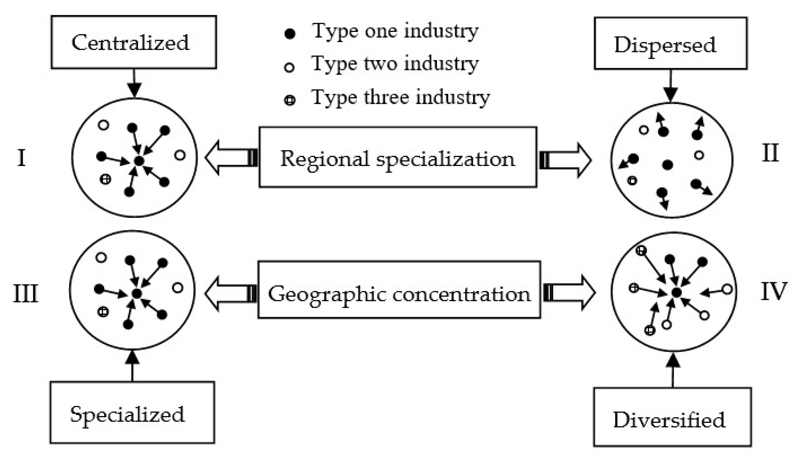
2.1. The Type of Agglomeration Externalities

The literature commonly distinguishes between regional specialization and geographic concentration with regard to agglomeration. The concept of specialization concerns the location of well-defined industries with a homogenous input structure in a region, while geographical concentration is defined as a group of business activities concentrated in a particular area [33,34]. As depicted in Figure 1, the first type of industry in a region is specialized in both Type I and Type II agglomeration, but they present different characteristics. The former is concentrated toward a particular point or around an area, whereas the latter is spatially dispersed. There are also two types of geographic concentration, i.e., specialization agglomeration (Type III) and diversification agglomeration (Type IV). Type III agglomeration is the same as Type I, as some industries in a region are both specialized and spatially concentrated. Type IV agglomeration means that many related or unrelated, and local advantaged or disadvantaged industries are clustered in an area. It is suggested that the greater specialization in a region of some advantaged industries does not necessarily result in a higher degree of geographical concentration [33]. In fact, an increase in specialization of type II (see Figure 1) results in a reduction in the spatial concentration level. For example, many members of the European Union, such as Belgium, Denmark, Greece, Austria, and Portugal, experienced an increase in specialization but decrease of concentration in the 1990s [35].
In our framework, the model of regional specialization development probably has an overlapping effect with geographic concentration, such as type I and type III agglomeration (see Figure 1). In this sense, the concepts of specialization and concentration can be used to explain the way agglomeration externalities occur [34,36,37]. However, the most pronounced difference is that specialization agglomeration pays more attention to how to develop a comparative advantage sub-industry in a region using the convergence strategy or decentralized strategy, while spatial concentration focuses on how to use spatial or geographical proximity to boost regional economic development using the specialized agglomeration or diversified agglomeration strategy. In short, the specialization mechanism is based on local comparative industry, while the concentration mechanism is based on geographical advantage. Therefore, the meaning of specialization and concentration should not be simply treated as being different sides of the same coin [33].
Despite the differences in opinion on the agglomeration mechanism, there is a general consensus in the literature that an industrial agglomeration zone or park is an important factor in explaining why local environment quality is different across regions [22,26,30]. In our study, the type of agglomeration mechanism is expected to have a nonlinear relationship with local haze pollution over time.

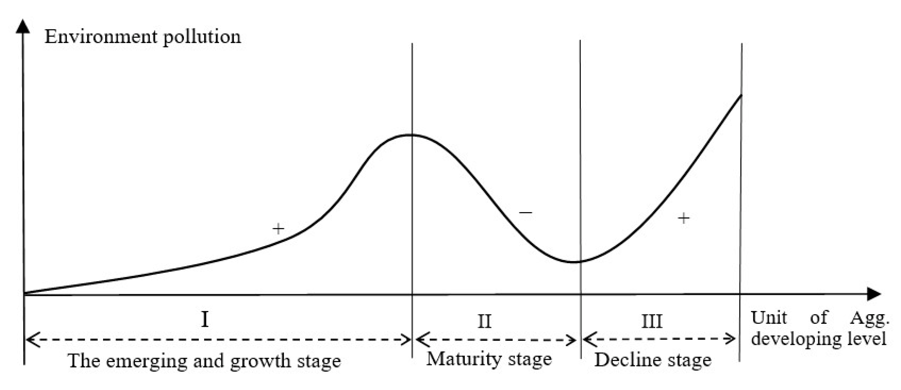
2.2. The Life Cycle of Agglomeration

The theory of the industry life cycle suggests that industries evolve according to the trajectory of birth, growth, maturity and decline. Many scholars use the theory of the industry life cycle to explain how the industrial clusters, cities, as well as regions evolve over time. For example, Martin and Sunley (2011) draw on the ‘adaptive cycle’ model to explore cluster evolution [38]. They suggest that cluster evolution is considered as an adaptive process of micro-behaviours, the agency and individuals, and firms and experiences in five stages, i.e., emergence, growth, maturation, decline, and eventual replacement by new cluster. Moreover, agglomeration is classified into three phases by Hayter and Edenh offer (2016), i.e., firms concentrated in the core, dispersal to the periphery and closure [39]. Similarly, Kim and Park (2015) suggest that industrial agglomeration mainly experiences three stages, i.e., birth, growth and maturity [40]. The classifications listed above are all generally in line with the evolutionary agglomeration theory. Based on the framework of Evolutionary Economic Geography and Potter and Watts’s research [41], we suggest that agglomeration experiences three basic stages of development, i.e., the birth and growth stage, mature stage, and decline stage.

2.3. Theoretical Hypothesis

It is suggested that agglomeration in different stages of development presents different spatial spillover effects in terms of resource allocation efficiency, R&D efficiency, competition and cooperation efficiency, and public facilities construction [41,42] In this paper, the type of agglomeration externalities is assumed to have a nonlinearly N-shaped impact on air pollution based on the theory of the life cycle. We draw a picture to further discuss the periodic change of agglomeration externalities impacting on environmental pollution (see Figure 2).
During the birth and growth stage, the effect imparted by centralization outweighs the decentralization effect, and the pattern of agglomeration is similar to type I agglomeration (see Figure 1). Enterprises can obtain increasing returns of agglomeration economies in this stage due to supply chain relevance or geographical proximity, such as decreased costs, tacit knowledge transferring, network connectivity, and so on. However, in the emerging and growth stage, local infrastructure and the environmental regulation mechanism are highly underdeveloped, leading to local resource allocation and utilization efficiency that are far from the optimal state. At the same time, firms clustering in an area result in high energy consumption, and an increase in carbon emissions, hence, worsening the urban environment [43,44]. Consequently, agglomeration in the early stage is expected to have a positive effect on environment pollution.
During the mature period, a number of mechanism changes occur. On the one hand, the knowledge among cluster’s firms becomes codified, standardized, and transferable across regions with low transaction costs [45]. Enterprises in the agglomeration zone can maintain knowledge and technology spillovers from local leading firms. By having a large number of skilled workers and innovative firms in the mature stage of agglomeration, the surrounding cluster area benefits from a significant increase of technology innovation and productivity. The increase in labour productivity is helpful for industrial energy efficiency improvement and further reduces carbon emission [46]. On the other hand, during the mature stage of agglomeration, regional infrastructure and the environmental protection mechanism are both improved, and more and more cleaner production technological innovation emerges, which is spread across regions. As a result, both the efficiency of resource allocation and the scale of agglomeration generally achieve the optimal state. As Cai et al. suggest [47], an initial cluster area dominated by capital-intensive and heavy industry is more likely to develop green technology due to an increasingly mature environmental protection mechanism in China. In this case, the agglomeration externalities evolving into the mature stage are expected to play a beneficial role in pollution reduction.
When agglomeration enters into the stage of decline, the congestion effect outweighs the agglomeration effect and causes a number of negative externalities, such as greater land rents, higher energy consumption and carbon emission. During this stage, firms within the agglomeration zone experience decreasing returns of agglomeration economies on the one hand but continue experiencing increasing returns from dispersion economies on the other [41]. In this sense, agglomeration is similar to the form of type II specialization, as depicted in Figure 2, or the form of decentralization with a variety industries. The excessive concentration of firms or people in a region can produce a crowding effect, leading to transaction cost raising, a decrease in energy efficiency, and intensive competition [48]. Particularly, excessive competition can result in a situation in which the local market becomes monopolized by a few large and leading firms, which is proven to be unfavorable for new business formation and for survival in or near the cluster [41]. In addition, in the decline stage of agglomeration, regional technology innovation incorporating green and recycling technology can become locked in the un-development level and the efficiency of resource relocation likely returns to the initial stage. As a consequence, the agglomeration in the decline stage dominated by the congestion effect is expected to generate a deteriorating effect on the environment.
In general, the idea of whether agglomeration externalities are considered to lead to the “pollution heaven” or to pollution reduction depends on the life cycle of agglomeration development. In this paper, we use haze pollution as the pollutant indicator to capture the environmental externalities that are probably caused by agglomeration economies. The development of agglomeration, whether of regional specialization or concentration, is expected to have a N-shaped effect on regional haze pollution over time.

3. Methodology

3.1. Empirical Model

Based on the STIRPAT model (Stochastic Impacts by Regression on Population, Affluence, and Technology) created by Dietz and Rosa [49], we developed a more general model to capture the effect of agglomeration externalities on haze pollution. The benchmark model is defined as:
H a z e i t = α × A g g i t δ × P i t θ × A i t τ × T i t ϕ × υ i t
where i and t denote the index of city and year, respectively. Hazeit, the dependent variable, denotes haze pollution; Aggit, the independent variable, represents agglomeration externalities which is distinguished between regional specialization and geographic concentration in the estimation; Pit, Ait, and Tit represents the number of population, the degree of affluence and technology innovation, respectively in city i and period t. α is the constant term, while εit is the stochastic error term. When Equation (1) is transformed into linear logarithmic form, the model can be derived as:
L n   H a z e i t = α 1 + δ   L n A g g i t + β L n X i t + μ i + η t + ε i t
where α1 is the constant term, μi is the city-specific fixed effect, ηt is the time-specific fixed effect. In order to investigate spatial spillover effects, we mainly use the spatial Durbin Model (SDM) to estimate the environmental externalities of agglomeration because haze pollution in a region may have spatial correlation with other regions. Moreover, in order to capture the dynamics of agglomeration, the items of Agg2 and Agg3 are added into Equation (2). Therefore, the final econometric model can be expressed as:
L n   H a z e i t = α 1 + 1 L n   H a z e i , t 1 + ρ 1 j = 1 n W i j   L n H a z e j t + δ 1 L n   A g g i t + ρ 2 j = 1 n W i j L n   A g g j t                                               + δ 2 L n ( A g g i t ) 2 + δ 3 L n ( A g g i t ) 3 + β L n X i t + μ i + η t + ε i t
where Wij represents a spatial weight matrix. Following traditional procedure in the literature (Fan and Xu., 2020; Fang et al., 2020; Li et al., 2021), we mainly use the standard binary geographical neighboring weight to conduct regressions. If two places are adjacent, the value of Wij is equal to 1, otherwise it is equal to 0. Furthermore, WijLnHazejt denotes the spatial correlation among the dependent variables (i.e., haze pollution) of each region. WijLnAggjt represents the spatial correlation among the independent variables (i.e., agglomeration externalities) of each region. Additionally, ρ1 represents the coefficient of spatial spillover effect of haze pollution, when ρ1 ≥ 0, it indicates that there is a positive spatial correlation. Similarly, ρ2 denotes the spatial correlation coefficient of industrial agglomeration. δ1 represents the coefficient of industrial agglomeration on haze pollution. If δ1 ≥ 0, δ2 ≤ 0, δ3 ≥ 0, there exists an N-shaped relationship between agglomeration economies and haze pollution. If δ1 ≤ 0, δ2 ≥ 0, δ3 ≤ 0, there is an inverted N-shaped relationship between agglomeration economies and haze pollution. If δ1 = 0, δ2 ≤ 0, δ3 ≥ 0, the relationship presents an inverted U-shaped characteristic. If δ1 = 0, δ2 = 0, δ3 ≠ 0, industrial agglomeration is positively or negatively correlated with haze pollution. X denotes a series of controlling factors, including the degree of affluence, industrial structure, urban green infrastructure, foreign direct investment, technology innovation, and fiscal decentralization. Lastly, β denotes the coefficients of the controls impacting on haze pollution.

3.2. Variables

3.2.1. Dependent Variable

The dependent variable, i.e., haze pollution, is measured using the value of PM2.5 concentration in the air. At present, scholars most often use carbon dioxide (CO2), sulfur dioxide, or API (air pollution index) as air pollutant indicators. The reason as to why we selected the index of PM2.5 concentration to measure the degree of local air pollution is that PM2.5 is more harmful for people’s health. Moreover, more than half of cities in China have a PM2.5 concentration level that does not satisfy the recommended standard of the World Health Organization. In order to obtain a more consistent result, the CO2 emission degree of both per square kilometer and per capita are also used as the substitute variables of the index of PM2.5 concentration.

3.2.2. Independent Variables

Drawing on the discussion above, we use regional specialization and geographic concentration as two independent variables in the paper. Following the previous studies [50,51], we use the location quotient (LQ) index to measure the specialization agglomeration. Regional specialization agglomeration in the context of manufacturing is defined as:
R e g i o n a l   s p e c i a l i z a t i o n = M a n u f a c t u r i n g   o u t p u t i / M a n u f a c t u r i n g   o u t p u t C i t y   o u t p u t i / C i t y   o u t p u t C h i n a
where i represents city; Manufacturing outputi is the output of manufacturing in city i; Manufacturing output represents national manufacturing output; City outputi denotes the GDP level in city i; City outputChina denotes the total GDP in China. The LQ indicator outlined in Equation (4) can represent the specialization agglomeration. We also use the local specialization level in the secondary industry to represent specialized agglomeration for robust tests.
We use labour density as a measurement of geographical concentration, which is common in the literature [32,52]. The geographical concentration of manufacturing is defined as:
G e o g r a p h i c   c o n c e n t r a t i o n = M a n u f a c t u r i n g   e m p l o y m e n t i C i t y   a r e a i
where manufacturing employmenti denotes employment in manufacturing at the city level; city area i denotes the land area in city i. This indicator is depicted in Equation (5), and can be used to calculate the level of manufacturing employment per unit land area, denoting the degree of spatial concentration of manufacturing. In the process of our robust analysis, we also applied the population density as another measure of geographic concentration externalities.

3.2.3. Control Variables

In accordance with previous studies [9,53,54,55], we controlled several potential factors as shown in Equation (3), i.e., the degree of affluence (GDP), industrial structure (Indus), urban green infrastructure (Green), foreign direct investment (FDI), technology innovation (Tec), and fiscal decentralization (Dec).
Following the EKC hypothesis, the degree of local affluence and industrial structure are considered to be two important factors impacting on environment pollution. We used GDP per capita to measure the degree of affluence, while the control of industrial structure was measured by the ratio of output value of tertiary industry to secondary industry. Moreover, the PHH theory postulates that regional foreign investment is expected to be an important mechanism to explain local environment pollution. In the paper, the control of FDI is measured by foreign investment per capita in the current year. According to the STIRPAT model, it is not appropriate to systematically detect the impact of agglomeration economies on pollution without considering the effect caused by technology innovation. In this case, we use R&D expenditure per capita to measure the control variable of technology innovation. Urban green infrastructure, in general, and urban forests and trees in particular, are widely expected to improve air quality by removing gaseous air pollutants and particulate matter [56]. In the regression, we use the urban green coverage rate of the built-up area to measure the degree of urban green infrastructure. Lastly, we control fiscal decentralization in the regression model. Fiscal decentralization is expected to act as a proxy measurement to represent local governments’ competition, including taxation competition and investment competition. We applied the share of local government fiscal revenue in total revenue to measure the level of fiscal decentralization.

3.3. Data

The raster data of PM2.5 was obtained from the Social Economic Data and Application Center (SEDAC) of Columbia University. Furthermore, we used the Arc GIS software to parse the raster data into the specific annual average PM2.5 concentration of 289 cities at the prefecture level in China. The unit used for the PM2.5 concentration index is μg/m3. The CO2 emission, population, manufacturing output and employment, secondary industry output, administrative land area, green coverage rate, foreign investment, R&D expenditure, the output value of both tertiary and secondary industry, as well as government fiscal revenue at the city level were all obtained from the China City Statistical Yearbook (1999–2020). The sample includes Chinese urban panel data for 289 cities during the period from 1998 to 2019. The reason that we selected 1998 as the starting year is that the data of PM2.5 before 1998 at the city level in China are quite difficult to obtain. Notably, the missing data in our sample were converted by moving average method. Table 1 shows descriptive statistics for all variables applied in our empirical research.

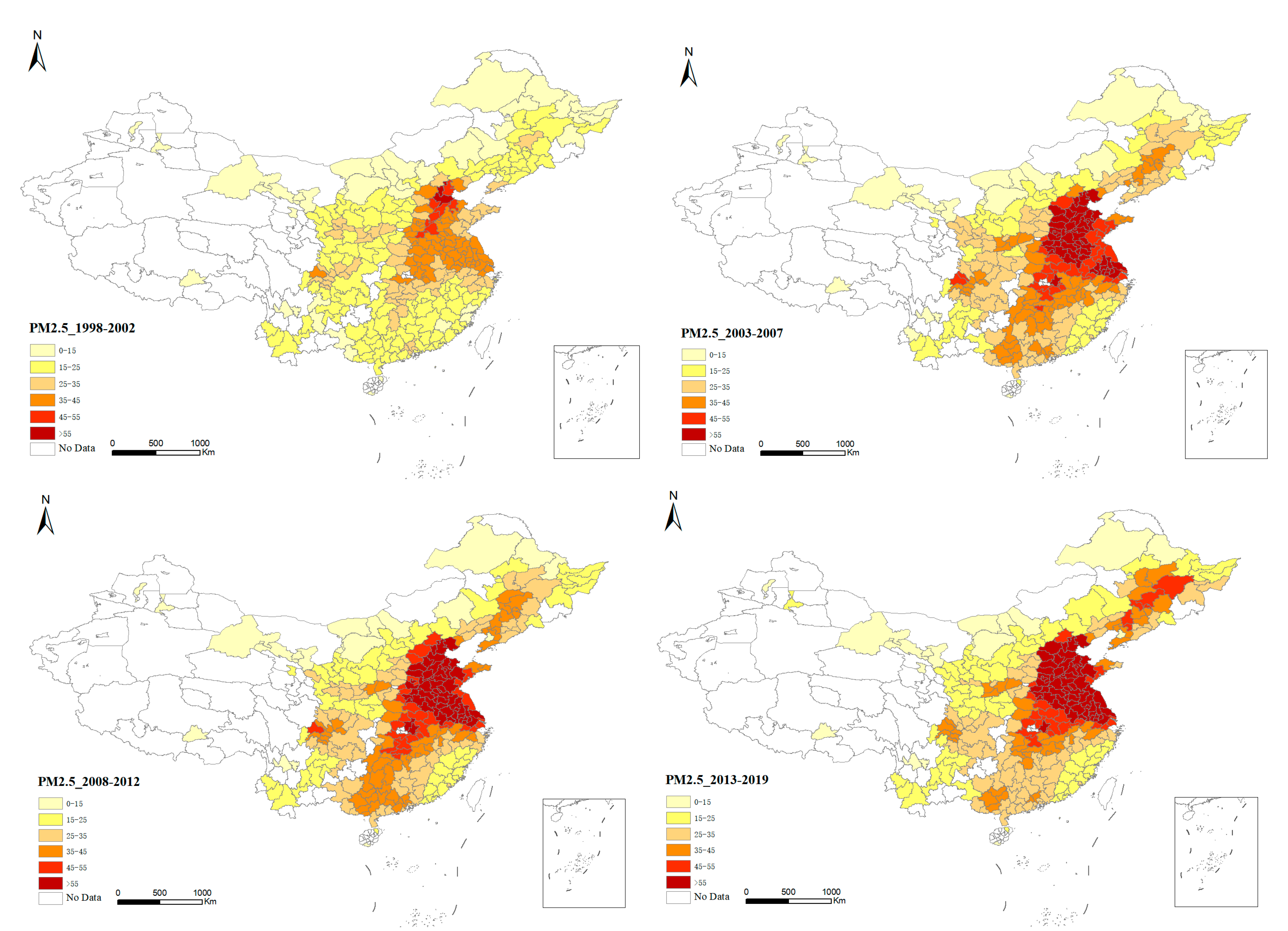
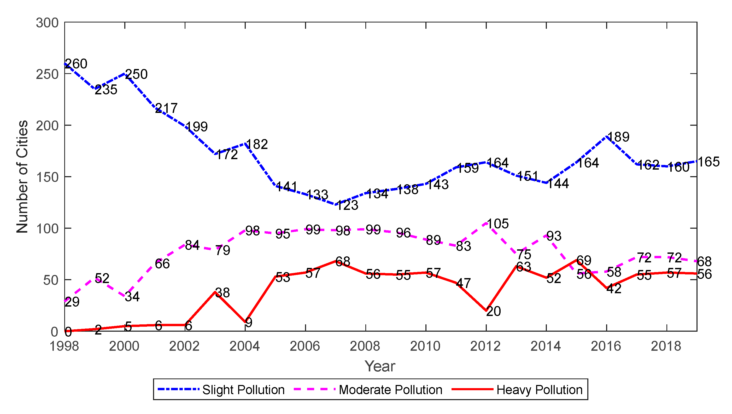
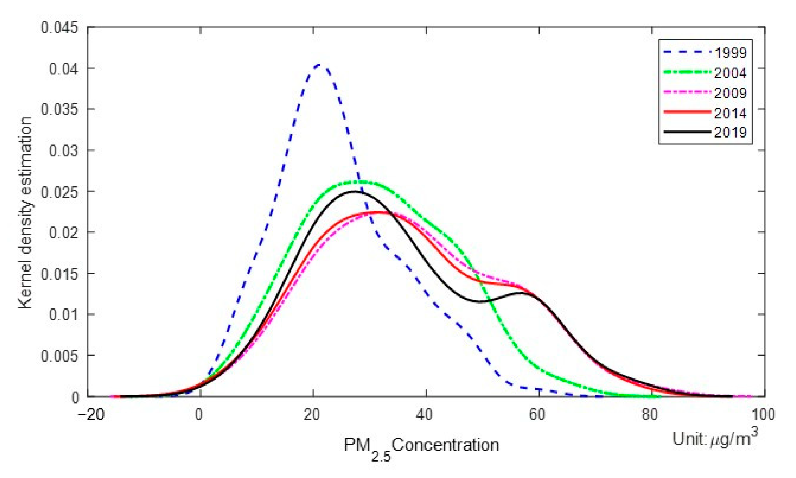
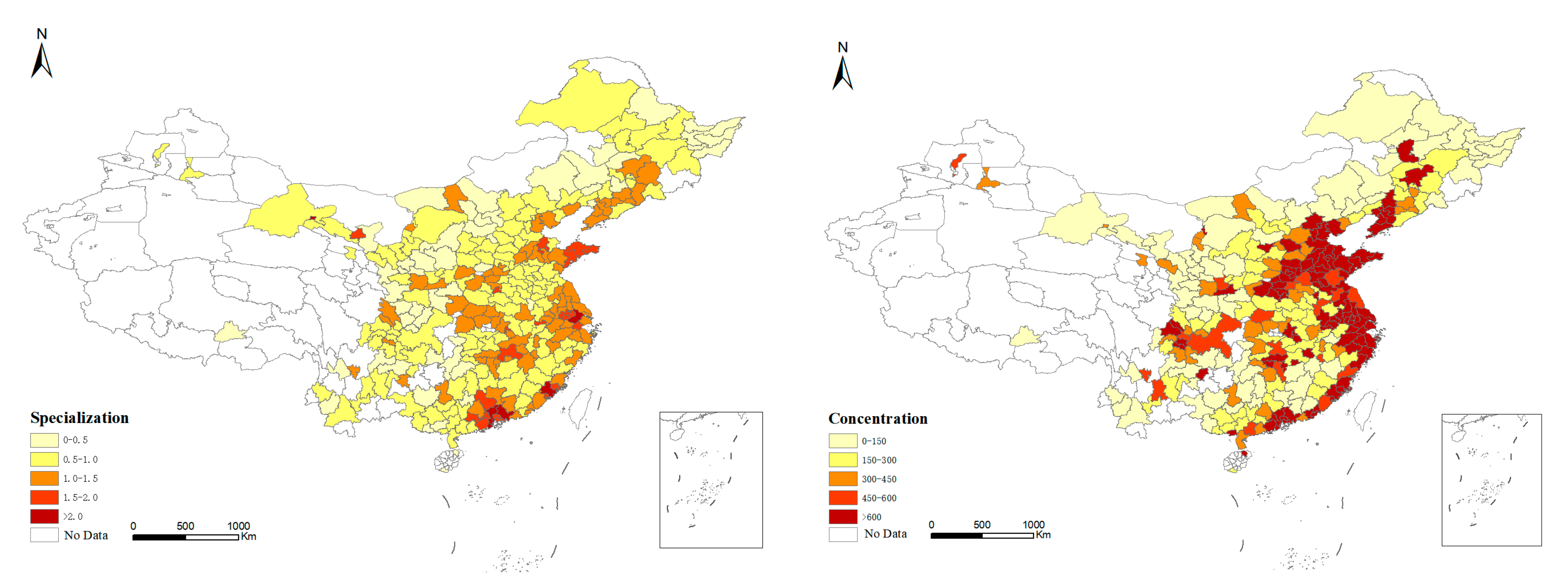
3.4. Spatial Difference of Haze Pollution and Industrial Agglomeration

We selected the years of 1998, 2003, 2008, 2013, and 2019 as the time points to depict the spatial distribution and the evolution of haze pollution at the city level. Figure 3 presents the dynamic and spatial distribution of haze pollution from 1998 to 2019 across China. As shown in Figure 3, the cities with the highest PM2.5 concentration in China, whether during the year of 1998–2002, 2003–2007, 2008–2012, or 2013–2019 are mainly located in the region of Beijing-Tianjin-Hebei, the Yangtze River Delta, and other provinces such as Shandong and Henan, while the lowest levels of PM2.5 concentration are found in Tibet, Heilongjiang, Inner Mongolia, Qinghai, Xingjiang, Gansu and other southwest provinces, such as Yunnan and Guizhou. Most cities in Fujian and the Guangdong province were also found to have a relatively low PM2.5 concentration. The spatial analysis indicates that haze pollution is distributed spatially unevenly across China. Considering the dynamic perspective, the results show that the number of the most polluted cities in China fluctuates during the period of 1998–2019. The area of the worst air pollution trends to decrease from 1998 to 2007, while, during the period of 2008–2019, it increases once again.
In addition, the most polluted areas seem to have been more and more spatially concentrated during the period of 1998–2019. Figure 3 also shows that the PM2.5 concentration in most cities of Sichuan, Hunan and Guangxi has dropped into the range of an acceptable standard, whereas the cities in or near the regions of Beijing-Tianjin-Hebei and the Yangtze River Delta still maintained a relatively higher level of PM2.5 concentration throughout the past two decades. The spatial analysis implies that current policies on haze pollution governance in a region are necessary to encourage cooperating with adjacent regions.
Additionally, we classify the samples of 289 cities as three groups in terms of the PM2.5 concentration index. If a city has a PM2.5 concentration of less than 35 μg/m3, it is defined as having slight haze pollution. Moderate pollution is classified as a PM2.5 concentration ranging from 35–55 μg/m3, while a city is classified as having heavy pollution if its PM2.5 concentration is more than 55 μg/m3. We calculated the number of cities in the three groups of haze pollution during the period of 1998 to 2019 (see Figure 4). It shows that the number of slight pollution cities has a decreasing trend, whereas the number of moderate and heavy pollution cities has increased significantly in the past decades. In addition, it reveals that there is a trade-off between the sight pollution and heavy pollution cites from 1998 to 2006, as well as during the period from 2015 to 2019, indicating that the years of 2006 and 2015 may be the turning point of haze pollution in urban China. To be specific, air quality in most cities presents a declining tendency over the period of 1998–2006, while the scope of moderate and heavy pollution seems to decrease significantly in the period from 2006 to 2016, indicating that urban haze pollution has been controlled and improved effectively in these years. However, after the year of 2016, the scope of moderate and heavy pollution cities seems to have expanded step by step, meaning that the air quality deteriorated again since then.
In order to further analyze the evolution of haze pollution across China, we estimated the kernel density distribution of haze pollution to explore the dynamic change of haze pollution (see Figure 5). In doing so, we found that the kernel density curve becomes steeper over time, indicating that haze pollution decreases as a whole and becomes concentrated in some areas. Such a concentration is shown to be reinforced gradually over time. Notably, the peak of distribution experiences decrease during the period of 2000–2012 and increased since 2012. In general, the kernel density distribution implies that China’s urban haze pollution is characterized by a strongly dynamic change.
Figure 6 presents the average value of regional specialization and geographical concentration across prefecture cities in China during the period of 1998–2018. It shows that industrial agglomeration, whether specialization or concentration, is distributed unevenly across China. At least a third of the sample cities in China have specialized manufacturing. In addition, the map on the left shows that the cities that specialize in manufacturing are not necessarily located in the coastal regions of China but are instead distributed in regional key cities and other resource-driven cities. In terms of geographical concentration, the map on the right shows that the distribution of manufacturing concentration basically follows the state of “low in the west and high in the east”. The concentration agglomeration measured by the employment manufacturing density in the coastal city is generally higher than that in the inner cities. However, some of regional key cities still account for a relatively high level of manufacturing concentration. For example, Chengdu, Chongqing, and Taiyuan, which are all located in inner region and regional key cities, possess a high level of manufacturing concentration. As a whole, the distribution of specialization and concentration agglomerations is roughly coherent with the spatial distribution of PM2.5 concentration across China.
In general, despite a slight increase in air quality over the past two decades, the most polluted cities display clustering in some areas such as the provinces of Hebei and Henan, as well as the Yangtze River Delta. By coincidence, the economic activities are quite active in such areas and agglomeration economics presents a stronger comparative advantage than other regions. Certainly, the industry structure in those polluted regions is mainly driven by heavy industry, as well as resource and energy industries, such as coal mines, the petrochemical industry, metallurgy and so on. Intuitionally, it can be observed that urban haze pollution in China changes dynamically over time and is strongly associated with specialization and concentration agglomeration.

4. Empirical Results

4.1. Spatial Correlation Analysis

The global Moran’s index generated by Moran (1950) is widely used to test the existence of the spatial correlation effect [57]. It can be defined as:
M o r a n s   I = i = 1 n j i n w i j ( x i x ¯ ) ( x j x ¯ ) s 2 i = 1 n j i n w i j
where xi denotes the variable in city i, x represents the mean value of xi, wij represents the spatial weight matrix, and n refers to the amount of cities. If the Moran’s index of haze pollution is more than 0, it means that the spatial correlation of haze pollution is positive, otherwise, the diffusion effect is supported. If the Moran’s index is equal to 0, it can be concluded that the spatial correlation effect does not exist.
Table 2 reports the results of Moran’s index of haze pollution during the period of 1998–2018. It shows that all of Moran’s indexes over time are positive and significant at the 1 percent level, suggesting that haze pollution in a city is spatially correlated with its adjacent cities. Moreover, the value of Moran’s index was found to have increased steadily during the past two decades. It implies that the spatial correlation of haze pollution among different cities is strengthened over time.

4.2. Baseline Estimation Results

Table 3 reports the empirical results of industrial agglomeration’s impact on haze pollution. The dynamic spatial Dubin Model estimates show that the coefficients of Agg and Agg3 are both positive and statically significant, while the coefficient of Agg2 is negative and significant at the 1% level (see column (3) and (6) in Table 3). In other words, the coefficients of δ1 and δ3 are more than 0, while the coefficient of δ2 is less than 0 as discussed in Section 2.1, indicating that the agglomeration externalities, when differentiating between regional specialization and geographical concentrations, has a significant N-shaped relationship with haze pollution.
In order to conduct a consistency test, on the one hand, we report the results by using Space Panel Lag model (see column (2) and (5)) and non-spatial model in Table 3 (see column (1) and (4)). It shows that the coefficients of Agg, Agg2 and Agg3 turn out to be quite consistent with the results conducted by SDM, indicating that the relationship between industrial agglomeration and haze pollution is indeed N-shaped. According to the fixed effect model, the values of geographical concentration with respect to the first and the second turning points is 1.2 and 10.47, respectively, while the values of regional specialization in terms of the first and the second turning points is 1.03 and 1.65, respectively. On the other hand, we retest the existence of the dynamic of agglomeration externalities and their impact on air pollution using 60 years’ time series data from 1960 to 2019. During the past 60 years, industry clusters or parks in most provinces in China experienced a development process from birth, growth to maturity and decline. Table 4 reports the empirical results of agglomeration externalities on air pollution over the past 60 years. In the regression model, concentration agglomeration is measured by the labor density of manufacturing. The measurement of specialization agglomeration seems to be somewhat complex. As a proxy measure, we used the efficiency of manufacturing to represent specialization agglomeration because the LQ index is usually used to calculate the degree of specialization in a particular area instead of specialization as a whole. In addition, the dependent variable of air pollution was measured by national carbon dioxide per capita as well as per unit area in the regression models. The results show that the coefficients of Agg and Agg3 are both positive and significant, while the coefficient of Agg2 turns out to be significantly negative, reconfirming that this type of industrial agglomerations has a N-curve relationship with air pollution over time.
The coefficients of neighboring haze pollution at the city level are all positive and significant at the 1% level in columns (2)–(3) and (5)–(6) in Table 3, indicating that haze pollution is indeed spatially correlated by the channel of imitation and learning effect among neighboring regions. The result is consistent with our analysis on the spatiotemporal evolution of haze pollution (see Figure 3). Some scholars also report a similar result. For example, Chen (2020) empirically suggests that air polluting industries prefer to cluster together in China, resulting in haze pollution that exhibits an obvious characteristics of clustering [58]. Interestingly, the spatial coefficient of geographical concentration turns out to be significantly positive in column (4), while the coefficient of the spatial weight matrix of regional specialization turns out to be negative and significant in column (6). Why is it that two types of agglomeration economies present an opposite effect on haze pollution of neighboring region? To respond to this question, it is necessary to consider the reality of the development of industrial agglomeration in China.
Each region in China tends to support and develop local comparative industries due to local resource availability as well as central-government coordination. In this context, industrial distribution between adjacent regions in China seems to be indented and complementary. Therefore, a region with a higher level of specialization has more of a spillover effect on its neighboring regions, in aspects such as technological progress, increases efficiency and environmental improvement. However, the industrial concentration generated by geographical proximity always presents a strong spatial competitiveness with neighboring regions [55]. There are two basic measures to develop geographical concentration applied by local governments in China. The first is to attract foreign direct investment clustering in local areas. The second is to expand or rebuild local industrial parks. In this case, the increase of industrial concentration in an area likely results in the decrease in industrial concentration in other adjacent regions. He et al. (2010) believe that the development of an industrial cluster led by local governments is likely to fall into the vicious circle of fierce as well as low-level competition among regions, resulting in hastening the construction of local industry and worsening the local environment [59]. Therefore, it makes sense that the development of geographical concentration in a region seems to generate negative externalities on neighboring air environments.

4.3. Heterogeneity Test of Different Groups of Cities

The general estimation results support the existence of the type of agglomeration externalities’ effect on haze pollution. However, for different group of cities, the effect of agglomeration economies on haze pollution cannot be similarly generalized. Table 5 reports the heterogeneity test results of three groups of cities based on the fixed effects model. According to the difference of urban population, we divided the sample of China’s 289 cities into three groups, i.e., mega-city, large city, as well as small and medium city. Generally, a mega-city has more than 100 million permanent residents, while a city with 1 to 100 million permanent residents is classified as a large city, and the rest of the cities in the sample are defined as small or medium cities. The mega-city in this paper is identical to the first-tier cities ranking in the China City Business Charm Ranking List, while the group of large cities are mostly the sum of the second-tier, third-tier and fourth-tier cities and other cities are classified as the small and medium city. The result shows that the coefficients of regional specialization and concentration are both positive and statistically significant in column (1) and (4) in Table 5, indicating that industrial agglomeration as a whole in a mega city has a positive effect on local haze pollution. This is probably due to the fact that current manufacturing agglomeration in most mega cities in China has entered into the decline stage dominated by the congestion effect, when agglomeration economies present a deteriorating effect on local air environment. This empirical result can explain the phenomenon of mega cities in China attempting to relocate the administrative center into an urban fringe area, such as Xiongan New Area in Beijing, Pudong New Area in Shanghai. The relocation of the administrative center in mega cities can encourage people and firms to move out of urban central areas, which is beneficial for decreasing urban congestion and improving urban air environment.
The result in large city group shows that the coefficients of Agg and Agg2 are significantly positive and negative, respectively in column (2), while, by contrast, the same coefficients in column (4) turn out to be reversed (see Table 5). It implies that the linkage between specialization and haze pollution seems to be nonlinearly U-shaped, while the geographical concentration presents an invested U-shaped effect on local haze pollution. An alternative explanation is that industrial concentration in most large cities of China has reached fast developing stages, while the specialization agglomeration in these cities has entered into the mature or decline stage. Following the curve of dynamic change of agglomeration externalities summarized in Figure 2, the development of concentration agglomeration during the first and second stages, as a whole, seems to present an invested U-shaped effect on haze pollution, whereas specialization agglomeration during the second and third stages shows a U-shaped relationship with haze pollution.
In terms of small and medium cities, the results show that the coefficient of concentration agglomeration is positive and significant in column (3), while the coefficient of specialization agglomeration is significantly negative in column (6) in Table 5. This indicates that the haze pollution in small and medium cities can be effectively reduced using a specialization strategy, but tends to deteriorate when subject to the concentration strategy. Currently, most small and medium cities in China are characterized as having a low population density and a low density of firms, and the development of their concentration agglomeration is generally at the early or decline stage (see Figure 2), which leads to a deteriorating effect on local haze pollution. However, the degree of regional specialization in small and medium cities is not necessarily lower than large cities. Approximately, the data show that more than a half of the small and medium cities in our sample have a manufacturing specialization index of more than 1, suggesting the specialization agglomeration in small and medium cities has crossed the early stage. In this case, the development of specialization in small and medium cities presents positive externalities in increasing air quality. The findings of the heterogeneous analysis seem to be mixed, but still generally confirm the existence of the life cycle of industrial agglomeration impacting on haze pollution in different type of cities.

4.4. Robustness Test

To improve the robustness of the results, we used several regression methods. First, we selected the GDP distance rather than the geographic distance as the weight matrix to re-estimate. The results are reported in Table 6. We found that the results are highly consistent with those presented in Table 3. To be specific, the coefficients of Agg and Agg3 for both specialization or concentration are all positive and significant, while the coefficient of Agg2 is significantly negative when controlling for other potential factors. The results conducted by the GDP distance weight matrix further underpin the abovementioned conclusions. Second, we applied the system generalized moment method (GMM) to estimate the pollution effect caused by agglomeration economies. The system GMM estimators with instrumental variables of lagged regional specialization and lagged geographic concentration are presented in column (1) and (4), respectively in Table 7. The results are consistent with the results conducted by spatial panel estimations, reconfirming that the development of agglomeration has a N-typed instead of simply positive or negative effect on haze pollution over time. Third, the replacing regression method was used for a further robustness test. On the one hand, we applied the population density to substitute for manufacturing employment density and used the LQ index of the secondary industry to substitute for manufacturing specialization in the lagged spatial and SDM models [see column (2) to (3) and (5) to (6) in Table 7]. On the other hand, we also reported the replacing regression results of SLM and SDM using the GDP distance matrix (see column (3) to (4) and (7) to (8) in Table 6). The results are proven to be quite robust and consistent, re-supporting the dynamic change of agglomeration externalities.
Moreover, we apply the system GMM to retest the heterogeneity analysis of different groups of cities, where the lagged independent variable is used as instrument variable (see Table 8). The GMM results is also consistent with the heterogeneity test in different groups of cities. To be specific, the concentration agglomeration in both mage and small city indeed presents a positive and significant effect on haze pollution, while such effect turns out to be inversely U-shaped in large city. Unlikely, the specialization agglomeration in mage city presents a positive and significant effect on haze pollution, whereas it shows a significantly negative effect in small and medium city as well as a U-shaped effect in large city.

5. Discussion

The agglomeration mechanism is believed to be different in terms of the difference between specialization externalities and concentration externalities. In this paper, we classified agglomeration through two types, i.e., regional specialization and geographical concentration. The specialization strategy focuses on the question of how to develop comparative advantage industries in a region, while the concentration strategy pays attention to the issue of how to simulate agglomeration economies by optimizing industrial distribution in space. Our empirical results suggest that the agglomeration strategies—whether by industry specialization or spatial concentration—both present an N-shaped effect on haze pollution over time. Specifically, the development of both regional specialization and geographical concentration shows negative externalities on air environment in its early and decline stages, while the positive externalities only occur in the mature stage. As a matter of fact, there are lots of studies focusing on the environmental externalities generated by industrial agglomeration, but the results are quite inconsistent in the existing research. For example, Liu et al. (2018) confirm that the impact of industrial agglomeration on pollution and ecological efficiency follows the inverted U-shaped relationship [23], while Hu et al. (2019) empirically point out that the increase of diversification is conducive to the decrease of sulfur-dioxide-emission intensity and the development of specialization produces industrial pollution emission [60]. The reason as to why the agglomeration externalities on the environment seem to be distinctive is probably due to the fact that previous studies ignored the important role played by periodic change of agglomeration externalities.
As our theoretical hypothesis depicts (see Figure 2), the reason why industrial agglomeration has a nonlinearly N-shaped rather than a positive or negative effect on haze pollution can be mainly attributed to the dynamics of agglomeration externalities over time. During the birth and growth stage, agglomeration attracts a number of firms that cluster in its area by providing increasing returns of agglomeration economies but local environmental regulation is highly under-developed and the efficiency of resource and energy consumption is still at the low level, resulting in a positive effect on haze pollution. When the agglomeration exceeds a certain degree and evolves into the mature stage, haze pollution can be reduced by agglomeration externalities such as with technology innovation effect and productivity growth effect [45,47]. However, during the petrify stage, the development of agglomeration once again deteriorates the local air environment due to its congestion effect, such as excessive competition and over-exploitation [48]. In this case, it is necessary to identify the particular developing stage of agglomeration externalities before aiming to decrease haze pollution using the channel of agglomeration strategies.
Unlike the general estimation test, the heterogeneity test revealed that two types of agglomeration externalities have a distinctive effect on haze pollution. It seems to be a paradox, but it still makes sense when considering both the type of cities and their developing stages. In terms of different urban systems, concentration agglomeration in most small and medium cities is in the early stage and its industry density is relatively low, but mega cities seem to be overcrowded in this regard. Most small and medium cities possess a mature manufacturing system of specialization, while in most mega cities the specialized agglomeration of manufacturing fluctuates and turns to decline. Accordingly, the development of concentration agglomeration in the group of small and medium cities present a negative effect on haze pollution, while the specialization agglomeration in these groups shows a positive externalities. It implies that the development of low density as well as sprawled urbanization has a deterioration effect on the air environment on the one hand, while, on the other hand, urbanization by developing regional comparative advantage industries—whether by centralization or dispersion—is beneficial for improving local air environment. This conclusion also can be supported by other research. For example, Zhao et al. (2019) empirically suggest that the larger the city size (e.g., a high-density but single-center city) the easier it is to reduce haze using the mechanisms of optimizing local industrial structure, improving traffic accessibility and stimulating green technology innovation of enterprises [61]. Due to the congestion effect, the type of industrial agglomeration in the group of mega cities is proven to have a negative effect on haze pollution. This means decreasing industry density or increasing industry diversity properly are useful methods by which mega cities can improve their air quality. Lastly, the relationship between industrial agglomeration and haze pollution is proven to be nonlinear in the group of large cites, meaning that large cities should recognize the difference of development stages of industrial agglomeration and stimulate its positive effect on air environment.
The robustness test shows that the result concerning the effect of the dynamics of agglomeration on haze pollution is robust and consistent by different estimations. The heterogeneity test shows that the relationship between the type of agglomeration and haze pollution seems to be uncertain in different groups of cities, but is generally consistent with the hypothesis of dynamic change of agglomeration externalities.

6. Conclusions

There are a number of studies discussing the relationship between industrial agglomeration and environmental pollution, but the impact of the life cycle of agglomeration externalities on air pollution is still under explored in the literature. Our study examined the temporal and spatial boundaries of agglomeration externalities that explain why the agglomeration at different life stages presents a distinctive effect on air pollution. We divided agglomeration into regional specialization and geographical concentration and separately examined the dynamic effect of the type of agglomeration on haze pollution based on China’s 289 prefecture-level cities during the period of 1998–2018. The result suggests that the agglomeration externalities—whether of specialization or concentration—have a, N-shaped and significant effect on haze pollution. More specifically, the development of agglomeration whether at its beginning or decline stages presents a positive and significant effect on haze pollution, while local haze pollution can be significantly reduced by driving agglomeration into the mature stage. The result of heterogeneity test seems to be vary in different groups of cities, but it is basically consistent with the hypothesis concerning the life cycle of agglomeration externalities impacting on the environment. The robustness test shows that the results are quite robust and consistent. This paper provides answers to the question of how to trade off the relationship between the development of agglomeration and environment pollution over time.
Our findings have important policy implications. First, a city aiming to curb its haze pollution should cooperate with its neighbors because haze pollution is proved to be spatially correlated. Second, it is necessary to identify the particular developing stage of agglomeration because the result supports that the air pollution-reducing effect only occurs when the agglomeration develops into the mature stage instead of the beginning stage or diseconomies stage. Third, the industrial policies of agglomeration in an area should consider the local carrying capacity of the environment and resources, and, at the same time, the difference of agglomeration strategies. We conclude that specialization agglomeration and concentration agglomeration have a distinctive effect on haze pollution in terms of different groups of cities. For example, the development of low density and sprawled urbanization have been proven to negatively affect air quality, whereas urbanization, together with regional comparative advantage industries, are beneficial for improving air quality. The agglomeration policies in different groups of cities should stimulate its positive externalities on air quality, thereby avoiding the negative effects.

Author Contributions

X.T.: Conceptualization, Investigation, Visualization, Formal analysis and Writing—original draft. W.Y.: Methodology, Writing—review and editing, Funding acquisition, Project administration, Supervision and Validation. S.W.: Resources, Data curation and Software. All authors have read and agreed to the published version of the manuscript.

Funding

This article was sponsored by the Special Project of Fujian Provincial Finance Department (Grant No. 2021848), the Social Science Planning Project of Fujian Province (Grant No. FJ2020B118) and Natural Science Foundation of Fujian Province in China (Grant No. 2020J01459).

Institutional Review Board Statement

Not applicable.

Informed Consent Statement

Not applicable.

Data Availability Statement

In this study, the data were mainly obtained from China City Statistical Yearbook and the Social Economic Data and Application Center (SEDAC) of Columbia University.

Acknowledgments

The authors would like to thank the editor and the anonymous referees for their comments and suggestions which were most useful in revising the paper. The authors also would like to acknowledge Yayun Wang and Guoyang Zhang for their kind help for the paper.

Conflicts of Interest

The authors declare that they have no know competing financial interests or personal relationships that could have appeared to influence the work reported in this paper.

References

  1. Fan, C.C.; Scott, A.J. Industrial Agglomeration and Development: A Survey of Spatial Economic Issues in East Asia and a Statistical Analysis of Chinese Regions. Econ. Geogr. 2003, 79, 295–319. [Google Scholar] [CrossRef]
  2. Ying, G. Globalization and Industry Agglomeration in China. World Dev. 2009, 37, 550–559. [Google Scholar]
  3. Hu, C.; Xu, Z.; Yashiro, N. Agglomeration and productivity in China: Firm level evidence. China Econ. Rev. 2015, 33, 50–66. [Google Scholar] [CrossRef]
  4. Tang, K.; Gong, C.; Wang, D. Reduction potential, shadow prices, and pollution costs of agricultural pollutants in China. Sci. Total Environ. 2016, 541, 42–50. [Google Scholar] [CrossRef]
  5. Wolde-Rufael, Y.; Idowu, S. Income distribution and CO2 emission: A comparative analysis for china and india. Renew. Sustain. Energy Rev. 2017, 74, 1336–1345. [Google Scholar] [CrossRef]
  6. Ministry of Ecology and Environment (MEE). Bulletin on China’s Ecological Environment. 2020. Available online: http://www.mee.gov.cn/xxgk2018/xxgk/xxgk15/202005/t20200507_777895.html (accessed on 31 July 2021). (In Chinese)
  7. Greenstone, M.; Hanna, R. Environmental regulations, air and water pollution, and infant mortality in India. Am. Econ. Rev. 2014, 104, 3038–3072. [Google Scholar] [CrossRef] [Green Version]
  8. Ebenstein, A.; Fan, M.; Greenstone, M.; He, G.; Zhou, M. New evidence on the impact of sustained exposure to air pollution on life expectancy from China’s Huai River policy. Proc. Natl. Acad. Sci. USA 2017, 114, 10384–10389. [Google Scholar] [CrossRef] [Green Version]
  9. Fan, M.; He, G.; Zhou, M. The winter choke: Coal-fired heating, air pollution, and mortality in china. J. Health Econ. 2020, 71, 102316. [Google Scholar] [CrossRef] [Green Version]
  10. Islam, M.S.; Larpruenrudee, P.; Saha, S.C.; Pourmehran, O.; Paul, A.R.; Gemci, T.; Collins, R.; Paul, G.; Gu, Y. How severe acute respiratory syndrome coronavirus-2 aerosol propagates through the age-specific upper airways. Phys. Fluids 2021, 33, 081911. [Google Scholar] [CrossRef]
  11. Grossman, G.M.; Krueger, A.B. Environmental impacts of a north American free trade agreement. CEPR Discuss. Pap. 1992, 8, 223–250. [Google Scholar]
  12. Chichilnisky, G. North-south trade and the global environment. Am. Econ. Rev. 1994, 84, 851–874. [Google Scholar]
  13. Copeland, B.R.; Taylor, M.S. North-South trade and the environment. Q. J. Econ. 1994, 109, 755–787. [Google Scholar] [CrossRef]
  14. Cole, M.A.; Elliott, R.J.; Okubo, T. Trade, environmental regulations and industrial mobility: An industry-level study of Japan. Ecol. Econ. 2010, 69, 1995–2002. [Google Scholar] [CrossRef] [Green Version]
  15. Sung, B.; Song, W.-Y.; Park, S.-D. How foreign direct investment affects CO2 emission levels in the Chinese manufacturing industry: Evidence from panel data. Econ. Syst. 2018, 42, 320–331. [Google Scholar] [CrossRef]
  16. Chen, B. Industrial agglomeration and the pollution haven hypothesis: Evidence from Chinese prefectures. J. Asia Pac. Econ. 2021. [Google Scholar] [CrossRef]
  17. Han, F.; Xie, R.; Lu, Y.; Fang, J.Y.; Liu, Y. The Effects of Urban Agglomeration Economies on Carbon Emissions: Evidence from Chinese Cities. J. Clean. Prod. 2018, 172, 1096–1110. [Google Scholar] [CrossRef]
  18. Kang, Y.-Q.; Zhao, T.; Yang, Y.-Y. Environmental Kuznets curve for CO2 emissions in China: A spatial panel data approach. Ecol. Indic. 2016, 63, 231–239. [Google Scholar] [CrossRef]
  19. Lin, F. Trade openness and air pollution: City-level empirical evidence from China. China Econ. Rev. 2017, 45, 78–88. [Google Scholar] [CrossRef]
  20. Dou, J.; Han, X. How does the industry mobility affect pollution industry transfer in China: Empirical test on Pollution Haven Hypothesis and Porter Hypothesis. J. Clean. Prod. 2019, 217, 105–115. [Google Scholar] [CrossRef]
  21. Zeng, D.-Z.; Zhao, L. Pollution havens and industrial agglomeration. J. Environ. Econ. Manag. 2009, 58, 141–153. [Google Scholar] [CrossRef] [Green Version]
  22. Virkanen, J. Effect of urbanization on metal deposition in the bay of Töölönlahti, Southern Finland. Mar. Pollut. Bull. 1998, 36, 729–738. [Google Scholar] [CrossRef]
  23. Liu, J.; Zhao, Y.; Cheng, Z.; Zhang, H. The Effect of Manufacturing Agglomeration on Haze Pollution in China. Int. J. Environ. Res. Public Health 2018, 15, 2490. [Google Scholar] [CrossRef] [Green Version]
  24. Chen, D.; Chen, S.; Jin, H. Industrial agglomeration and CO2 emissions: Evidence from 187 Chinese prefecture-level cities over 2005–2013. J. Clean. Prod. 2018, 172, 993–1003. [Google Scholar] [CrossRef]
  25. Dai, P.; Lin, Y. Should There Be Industrial Agglomeration in Sustainable Cities? A Perspective Based on Haze Pollution. Sustainability 2021, 13, 6609. [Google Scholar] [CrossRef]
  26. Fang, J.; Tang, X.; Xie, R.; Han, F. The effect of manufacturing agglomerations on smog pollution. Struct. Chang. Econ. Dyn. 2020, 54, 92–101. [Google Scholar] [CrossRef]
  27. Zhu, Y.; Xia, Y. Industrial agglomeration and environmental pollution: Evidence from China under New Urbanization. Energy Environ. 2018, 30, 1010–1026. [Google Scholar] [CrossRef]
  28. Gao, L.; Li, F.; Zhang, J.; Wang, X.; Hao, Y.; Li, C.; Tian, Y.; Yang, C.; Song, W.; Wang, T. Study on the Impact of Industrial Agglomeration on Ecological Sustainable Development in Southwest China. Sustainability 2021, 13, 1301. [Google Scholar] [CrossRef]
  29. Glaeser, E.L.; Kahn, M.E. The greenness of cities: Carbon dioxide emissions and urban development. J. Urban Econ. 2011, 67, 404–418. [Google Scholar] [CrossRef] [Green Version]
  30. Clark, L.P.; Millet, D.B.; Marshall, J.D. Air Quality and Urban Form in U.S. Urban Areas: Evidence from Regulatory Monitors. Environ. Sci. Technol. 2011, 45, 7028–7035. [Google Scholar] [CrossRef] [PubMed]
  31. Pei, Y.; Zhu, Y.; Liu, S.; Xie, M. Industrial agglomeration and environmental pollution: Based on the specialized and diversified agglomeration in the Yangtze River Delta. Environ. Dev. Sustain. 2021, 23, 4061–4085. [Google Scholar] [CrossRef]
  32. Ciccone, A. Agglomeration effects in Europe. Eur. Econ. Rev. 2002, 46, 213–227. [Google Scholar] [CrossRef] [Green Version]
  33. Aiginger, K.; Davies, S.W. Industrial Specialisation and Geographic Concentration: Two Sides of the Same Coin? Not for the European Union. J. Appl. Econ. 2004, 7, 231–248. [Google Scholar] [CrossRef] [Green Version]
  34. Ceapraz, I.L. The Concepts of Specialisation and Spatial Concentration and the Process of Economic Integration: Theoretical Relevance and Statistical Measures. The Case of Romania’s Regions. Rom. J. Reg. Sci. 2008, 2, 68–93. [Google Scholar]
  35. Rossi-Hansberg, E.A. Spatial Theory of Trade. Am. Econ. Rev. 2005, 95, 1464–1491. [Google Scholar] [CrossRef] [Green Version]
  36. Zheng, D.; Kuroda, T. The impact of economic policy on industrial specialization and regional concentration of China’s high-tech industries. Ann. Reg. Sci. 2013, 50, 771–790. [Google Scholar] [CrossRef]
  37. Yu, W. Creative industries agglomeration and entrepreneurship in China: Necessity or opportunity? Ind. Innov. 2020, 27, 420–443. [Google Scholar] [CrossRef]
  38. Martin, R.; Sunley, P. Conceptualizing Cluster Evolution: Beyond the Life Cycle Model? Reg. Stud. 2011, 45, 1299–1318. [Google Scholar] [CrossRef]
  39. Hayter, R.; Edenhoffer, K. Evolutionary geography of a mature resource sector: Shakeouts and shakeins in British Columbia’s forest industries 1980 to 2008. Growth Chang. 2016, 47, 497–519. [Google Scholar] [CrossRef]
  40. Kim, G.H.; Park, I.K. Agglomeration economies in knowledge production over the industry life cycle: Evidence from the ICT industry in the Seoul Capital Area, South Korea. Int. J. Urban Sci. 2015, 19, 400–417. [Google Scholar] [CrossRef]
  41. Potter, A.; Watts, H.D. Evolutionary agglomeration theory: Increasing returns, diminishing returns, and the industry life cycle. J. Econ. Geogr. 2011, 11, 417–455. [Google Scholar] [CrossRef] [Green Version]
  42. Neffke, F.; Henning, M.; Boschma, R.; Lundquist, K.J.; Olander, L.O. The dynamics of agglomeration externalities along the life cycle of industries. Reg. Stud. 2011, 45, 49–65. [Google Scholar] [CrossRef] [Green Version]
  43. Parikh, J.; Shukla, V. Urbanization, energy use and greenhouse effects in economic development: Results from a cross-national study of developing countries. Glob. Environ. Chang. 1995, 5, 87–103. [Google Scholar] [CrossRef]
  44. Verhoef, E.T.; Nijkamp, P. Externalities in urban sustainability: Environmental versus localization-type agglomeration externalities in a general spatial equilibrium model of a single-sector monocentric industrial city. Ecol. Econ. 2002, 40, 157–179. [Google Scholar] [CrossRef] [Green Version]
  45. Bathelt, H.; Malmberg, A.; Maskell, P. Clusters and knowledge: Local buzz, global pipelines and the process of knowledge creation. Prog. Hum. Geogr. 2004, 28, 31–56. [Google Scholar] [CrossRef]
  46. Fan, X.; Xu, Y. Convergence on the haze pollution: City-level evidence from China. Atmos. Pollut. Res. 2020, 11, 141–152. [Google Scholar] [CrossRef]
  47. Cai, X.; Zhu, B.; Zhang, H.; Li, L.; Xie, M. Can direct environmental regulation promote green technology innovation in heavily polluting industries? Evidence from Chinese listed companies. Sci. Total Environ. 2020, 746, 140810. [Google Scholar] [CrossRef] [PubMed]
  48. Combes, P.P.; Gilles, D.; Gobillon, L.; Puga, D.; Roux, S. The productivity advantages of large cities: Distinguishing agglomeration from firm selection. Econometrica 2012, 80, 2543–2594. [Google Scholar] [CrossRef]
  49. Dietz, T.; Rosa, E.A. Rethinking the Environmental Impacts of Population, Affluence and Technology. Hum. Ecol. Rev. 1994, 1, 277–300. [Google Scholar]
  50. Markusen, A. Urban Development and the Politics of a Creative Class: Evidence from a Study of Artists. Environ. Plan. A Econ. Space 2006, 38, 1921–1940. [Google Scholar] [CrossRef] [Green Version]
  51. Delgado, M.; Porter, M.E.; Stern, S. Clusters and entrepreneurship. J. Econ. Geogr. 2010, 10, 495–518. [Google Scholar] [CrossRef]
  52. Andersson, R.; Quigley, J.M.; Wilhelmsson, M. Agglomeration and the spatial distribution of creativity. Pap. Reg. Sci. 2005, 84, 445–464. [Google Scholar] [CrossRef] [Green Version]
  53. Bai, Y.; Deng, X.; Gibson, J.; Zhao, Z.; Xu, H. How does urbanization affect residential CO2 emissions? An analysis on urban agglomerations of China. J. Clean. Prod. 2019, 209, 876–885. [Google Scholar] [CrossRef]
  54. Lu, W.; Tam, V.W.; Du, L.; Chen, H. Impact of industrial agglomeration on haze pollution: New evidence from Bohai Sea Economic Region in China. J. Clean. Prod. 2021, 280, 124414. [Google Scholar] [CrossRef]
  55. Hong, Y.; Lyu, X.; Chen, Y.; Li, W. Industrial agglomeration externalities, local governments’ competition and environmental pollution: Evidence from Chinese prefecture–level cities. J. Clean. Prod. 2020, 277, 123455. [Google Scholar] [CrossRef]
  56. Weber, C. Ecosystem services provided by urban vegetation: A literature review. In Urban Environment; Rauch, S., Morrison, G., Norra, S., Schleicher, N., Eds.; Springer: Dordrecht, The Netherlands, 2013; pp. 119–131. [Google Scholar]
  57. Moran, P.A.P. Notes on continuous stochastic phenomena. Biometrika 1950, 37, 17–23. [Google Scholar] [CrossRef]
  58. Chen, C.; Sun, Y.; Lan, Q.; Jiang, F. Impacts of industrial agglomeration on pollution and ecological efficiency-A spatial econometric analysis based on a big panel dataset of China’s 259 cities. J. Clean. Prod. 2020, 258, 120721. [Google Scholar] [CrossRef]
  59. He, C.; Zhu, Y.; Zhu, S. Industrial Attributes, Provincial Characteristics and Industrial Agglomeration in China. Acta Geograph. Sin. 2010, 65, 1218–1228. [Google Scholar] [CrossRef]
  60. Hu, Z.Q.; Miao, C.H.; Yuan, F. Impact of industrial spatial and organizational agglomeration patterns on industrial So2 emissions of prefecture-level cities in china. Acta Geogr. Sin. 2019, 74, 2045–2061. [Google Scholar]
  61. Zhao, X.; Shang, Y.; Song, M. What kind of cities are more conducive to haze reduction: Agglomeration or expansion? Habitat Int. 2019, 91, 102027. [Google Scholar] [CrossRef]
Figure 1. Different types of industrial agglomeration.
Sustainability 14 00580 g001
Figure 2. The N-shaped relationship between agglomeration and environment pollution.
Sustainability 14 00580 g002
Figure 3. Spatiotemporal evolution of PM2.5 concentration at the city level in China (μg/m3). Data source: The raster data of PM2.5 were obtained from the Social Economic Data and Application Center (SEDAC) of Columbia University.
Sustainability 14 00580 g003
Figure 4. The number of cites by three groups of haze pollution in China.
Sustainability 14 00580 g004
Figure 5. Estimated kernel density distribution of PM2.5 concentration in China.
Sustainability 14 00580 g005
Figure 6. Spatial distribution of specialization and concentration from 1998 to 2018.
Sustainability 14 00580 g006
Table 1. Descriptive analysis of the variables (1998–2019).
VariablesDefinitionMeanMaxMinStd. Dev.Obs.
HazePM2.5 concentration (μg/m3)33.2690.862.0215.776358
Agg1Manufacturing employment density
(People per square kilometer)
1622.40134,715.901.764956.376358
Agg2Population density (People per square kilometer)415.032310.564.70310.856358
Agg3LQ indicator of manufacturing0.9914.410.040.576358
Agg4LQ indicator of secondary industry0.9218.810.010.816358
GDPGDP per capita (Yuan per capita)32,978.90329,095.90965.8637,478.716358
IndusThe ratio of tertiary industry output to secondary industry (%)0.929.480.090.496358
GreenUrban greening rate (%)34.9796.150.1210.186358
FDIForeign investment per capita (Yuan per capita)842.0319,868.530.091720.576358
TecR&D expenditure level (Yuan per capita)101.8012,471.500.00382.836358
DecThe share local government fiscal revenue (%)33.0197.530.6520.006358
Notes: The variables of Agg1 and Agg2 are together used to denote geographic agglomeration, while the variables of Agg3 and Agg4 are together applied to denote specialization agglomeration.
Table 2. Moran’s I index of haze pollution during the period of 1998–2019.
YearHaze PollutionZ-ValueYearHaze PollutionZ-Value
19980.484 ***37.51920090.592 ***45.759
19990.484 ***37.50120100.662 ***51.162
20000.577 ***44.72220110.641 ***49.565
20010.589 ***45.63020120.611 ***47.225
20020.596 ***46.06520130.681 ***52.654
20030.692 ***53.52920140.630 ***48.716
20040.557 ***43.09320150.669 ***51.677
20050.600 ***46.4120160.704 ***54.469
20060.606 ***46.90920170.545 ***42.241
20070.706 ***54.53720180.582 ***45.375
20080.615 ***47.52520190.743 ***57.400
Notes: *** denotes statistical significance at the 1% level.
Table 3. Baseline estimation results.
VariablesGeographical ConcentrationRegional Specialization
FESLMSDMFESLMSDM
(1)(2)(3)(4)(5)(6)
Agg30.04 ***
(2.57)
2.00 **
(1.91)
0.14 *
(1.45)
0.03 ***
(6.80)
0.35 **
(1.98)
0.07 **
(2.33)
Agg2−0.46 *
(−1.81)
−38.44 ***
(−2.46)
−2.56 *
(−1.72)
−0.36 ***
(−7.15)
−5.13 **
(−2.03)
−0.98 **
(−2.35)
Agg2.88 **
(2.61)
183.27 ***
(5.27)
26.74 ***
(7.69)
1.60 ***
(7.03)
23.02 **
(1.94)
5.28 ***
(2.70)
Constant26.03 ***
(48.66)
−239.97 ***
(−22.39)
−318.17 ***
(−22.49)
1.66 ***
(4.86)
−15.00 **
(−2.01)
22.78 **
(1.97)
ControlsYesYesYesYesYesYes
W×Haze0.24 ***
(1.3 × 10⁵)
0.27 ***
(8.9 × 10⁴)
0.24 ***
(1.0 × 10⁵)
0.27 ***
(7.9 × 10⁴)
W×Agg3.27 ***
(5.04)
−0.21 ***
(−89.73)
R2/sigma2_e0.13−2.71 ***
(−103.37)
−2.67 ***
(−102.75)
0.211.91 ***
(21.31)
3.19 ***
(19.32)
Obs.635863586358635863586358
Notes: (a) FE, fixed effect; SLM, space panel lag model; SDM, spatial Durbin model; (b) The geographic distance matrix is selected as the weight matrix; (c) Control variables include the level of economic development, industrial structure, urban green infrastructure, foreign direct investment, technology innovation and fiscal decentralization; (d) *, ** and *** represent statistical significance at the 10%, 5%, and 1% levels, respectively, and z-statistics are shown in the parenthesis.
Table 4. The results of the impact of industrial agglomeration on air pollution (1960–2019).
VariablesGeographical ConcentrationRegional Specialization
(1)(2)(3)(4)
Agg36.41 ** (2.34)6.41 ** (2.34)0.02 *** (3.98)0.03 *** (5.00)
Agg2−84.79 ** (−2.23)−84.79 ** (−2.23)−0.27 *** (−3.93)−0.36 *** (−5.37)
Agg374.12 ** (2.12)376.12 ** (2.13)1.48 *** (5.62)2.08 *** (8.10)
Constant−555.45 ** (−2.04)−5555.45 ** (−2.04)−2.25 *** (−7.27)1.26 *** (4.19)
ControlsYesYesYesYes
R20.9500.9690.9750.985
Obs.60606060
Notes: Geographical concentration is measured by national level of labor density of manufacturing in column (1) and (2), while regional specialization is measured by the share of manufacturing output in its employment in column (3) and (4). The dependent variable is measured, respectively by CO2 emission per capita in column (1) and (3) as well as by CO2 emission density in column (2) and (4). All data is logarithmic. Other notes is the same as shown in Table 3.
Table 5. The results of heterogeneity test in three groups of cities.
VariablesGeography ConcentrationRegional Specialization
Mega CityLarge CitySmall m CityMega CityLarge CitySmall m City
Agg2−0.02 ***
(−8.12)
0.18 ***
(10.74)
Agg0.08 **
(2.27)
0.40 ***
(32.59)
0.37 ***
(44.48)
0.05
(0.98)
−1.80 ***
(−11.49)
−0.13 ***
(4.53)
Constant4.19 ***
(11.80)
4.46 ***
(45.90)
3.44 ***
(31.91)
4.45 ***
(9.05)
3.02
(0.77)
3.68 ***
(16.06)
ControlsYesYesYesYesYesYes
R20.090.410.590.090.190.14
Obs.19 × 22191 × 2279 × 2219 × 22191 × 2279 × 22
RelationshipPositiveInvested-UPositivePositiveU shapedNegative
Notes: The estimations are all based on the fixed effects model. Small m city, small and medium city. Other notes is the same as shown in Table 3.
Table 6. Robustness test results by GDP distance weight matrix.
VariablesGeographical ConcentrationRegional Specialization
SLMSDMSLMSDMSLMSDMSLMSDM
(1)(2)(3)(4)(5)(6)(7)(8)
Agg32.00 **
(1.91)
0.14 *
(1.45)
0.21 ***
(3.72)
0.02 *
(1.69)
0.35 **
(1.98)
0.07 **
(2.33)
0.10 ***
(2.75)
0.08 **
(1.88)
Agg2−38.44 ***
(−2.46)
−2.56 *
(−1.72)
−0.56 ***
(−3.21)
−0.03 *
(−1.84)
−5.13 **
(−2.03)
−0.98 **
(−2.35)
−1.38 ***
(−3.30)
−0.52 *
(−1.95)
Agg183.27 ***
(5.27)
26.74 ***
(7.69)
2.05 ***
(3.61)
5.53 **
(52.49)
23.02 **
(1.94)
5.28 ***
(2.70)
5.28 ***
(3.22)
2.07 **
(1.82)
Constant−239.97 ***
(−22.39)
−318.17 ***
(−22.49)
−55.71 ***
(−44.23)
0.36
(0.29)
−15.00 **
(−2.01)
22.78 **
(1.97)
−70.06 ***
(−23.58)
−151.15 ***
(−53.42)
ControlsYesYesYesYesYesYesYesYes
W×Haze0.24 ***
(1.3 × 10⁵)
0.27 ***
(8.9 × 10⁴)
0.27 ***
(2.2 × 10⁵)
0.27 ***
(1.4 × 10⁵)
0.24 ***
(1.0 × 10⁵)
0.27 ***
(7.9 × 10⁴)
0.27 ***
(2.3 × 10⁵)
0.27 ***
(1.9 × 10⁵)
W×Agg2.98 ***
(13.40)
0.89 ***
(117.74)
−0.21 ***
(−89.73)
−0.24 ***
(−62.82)
sigma2_e−2.71 ***
(−103.37)
−2.67 ***
(−102.75)
10.27 ***
(48.96)
6.93 ***
(54.40)
−3.63 ***
(−137.12)
−1.32 ***
(−16.21)
6.95 ***
(50.74)
5.10 ***
(65.49)
Obs.63586358635863586358635863586358
Notes: Geographical concentration is measured by the employment density of manufacturing in column (1) and (2), while it is measured by regional population density in column (3) and (4). Regional specialization is measured by the LQ index of manufacturing output in column (5) and (6), while it is measured by the LQ index of the secondary industry output in column (7) and (8). The GDP distance matrix is selected as the weight matrix, and other notes is the same as shown in Table 3.
Table 7. Robustness test results of general estimation.
VariablesGeography ConcentrationRegional Specialization
Sys-GMM
(1)
SLM
(2)
SDM
(3)
Sys-GMM
(4)
SLM
(5)
SDM
(6)
Haze(t−1)0.64 ***
(1157.31)
0.55 ***
(231.41)
Agg30.001 ***
(4.15)
0.18 ***
(3.26)
0.13 ***
(4.04)
0.002 ***
(2.78)
0.09 *
(1.38)
0.03 ***
(3.26)
Agg2−0.02 ***
(−25.54)
−0.51 ***
(−3.22)
−0.52 ***
(−4.96)
−0.03 ***
(−3.03)
−1.33 *
(−1.80)
−0.29 **
(−1.92)
Agg0.07 ***
(31.85)
5.32 ***
(12.57)
1.42 ***
(4.52)
0.12 ***
(2.91)
5.69 **
(2.05)
0.88 ***
(3.14)
Constant1.28 ***
(622.57)
0.18 ***
(3.26)
0.13 ***
(4.04)
2.44 ***
(40.53)
−27.22 ***
(−28.18)
−45.24 ***
(−15.21)
ControlsYesYesYesYesYesYes
W×Haze/AR(1)0.0010.24 ***
(1.1 × 10⁵)
0.24 ***
(1.2 × 10⁵)
0.0050.24 ***
(9.9 × 10⁴)
0.24 ***
(1.0×10⁵)
W×Agg/AR(2)0.210.12 ***
(11.39)
0.19−0.44 ***
(−52.93)
Sargan/sigma2_e1.002.42 ***
(19.60)
1.81 ***
(22.64)
1.002.00 ***
(21.31)
1.74 ***
(26.18)
Obs.606963586358606963586358
Notes: Sys-GMM, system generalized moment method; AR(1) and AR(2) denote Arellano-Bond autocorrelation tests of orders 1 and 2, respectively; Sargan is a test of the over-identifying restrictions for the GMM estimators; ‘t−1’ denotes that the variable in the estimations has been lagged by a year. Other notes is the same as shown in Table 3.
Table 8. Robustness test results by three groups of cities.
VariablesGeography ConcentrationRegional Specialization
Mega CityLarge CitySmall m CityMega CityLarge CitySmall m City
Haze(t−1)0.72 ***
(31.55)
0.67 ***
(823.96)
0.51 ***
(80.81)
0.78 ***
(68.19)
0.67 ***
(2136.08)
0.58 ***
(170.30)
Agg2 −0.004 ***
(−5.72)
0.01 ***
(6.75)
Agg0.03 *
(1.33)
0.06 ***
(11.13)
0.03 ***
(2.73)
0.03 *
(1.76)
−0.07 ***
(−4.15)
−0.02 **
(−2.47)
Constant0.84 **
(7.81)
1.42 ***
(108.62)
2.39 ***
(43.73)
0.72 ***
(10.88)
1.15 ***
(27.36)
1.16 ***
(29.49)
ControlsYesYesYesYesYesYes
AR(1)0.00100000
AR(2)0.060.210.260.040.080.03
Sargan1.000.961.001.000.961.00
Obs.19 × 21191 × 2179 × 2119 × 21191 × 2179 × 21
RelationshipPositiveInverted-UPositivePositiveU shapedNegative
Notes: The estimations are all based on the system generalized moment method. Small m city, small and medium city. Other notes is the same as shown in Table 3.
Publisher’s Note: MDPI stays neutral with regard to jurisdictional claims in published maps and institutional affiliations.

