Article

A Study on Near Real-Time Carbon Emission of Roads in Urban Agglomeration of China to Improve Sustainable Development under the Impact of COVID-19 Pandemic

1
State Key Joint Laboratory of Environment Simulation and Pollution Control, School of Environment, Beijing Normal University, Beijing 100875, China
2
Beijing Engineering Research Center for Watershed Environmental Restoration & Integrated Ecological Regulation, Beijing 100875, China
3
School of Environmental Science and Engineering, Shanghai Jiao Tong University, Shanghai 200240, China
4
Beijing Climate Change Management Centre, Beijing Municipal Environmental Protection Bureau, Beijing 100086, China
5
Department of Economics and Management, University of Florence, Via delle Pandette 9, 50127 Firenze, Italy
*
Author to whom correspondence should be addressed.
Sustainability 2022, 14(1), 385; https://doi.org/10.3390/su14010385
Submission received: 6 December 2021 / Revised: 24 December 2021 / Accepted: 28 December 2021 / Published: 30 December 2021
(This article belongs to the Special Issue Cleaner Production Practices and Sustainable Development)

Abstract

:
In order to achieve the goal of carbon neutrality and explore the impact of COVID-19 on urban road carbon emission, this study applied and improved a near real-time road carbon emission estimation method for typical Chinese urban agglomeration to improve the rapid evaluation of sustainable development. As a result, we recorded the daily road carbon emission for 12 cities in the Beijing–Tianjin–Hebei (JJJ) region under the impact of the epidemic, exploring the road carbon reduction effect caused by COVID-19. Singular value decomposition method was used to analyze the temporal and spatial characteristics of road carbon emission changes among cities and to explore the urban resilience oriented to public events. The results show: (1) In the JJJ region, the carbon reduction effect caused by COVID-19 is significant, but it lasted for a short time. In the three periods—before the epidemic, strict lockdown period, and post-lockdown period for prevention and control—the total daily road carbon emissions in the 12 cities were 170,000–190,000 tons, 90,000–110,000 tons, and 160,000–180,000 tons, respectively. (2) Cities in the JJJ region showed different road carbon reduction potential under short-term administrative control. During the “strict lockdown period” (23 January–25 February 2020), the average change rate of road carbon emissions in Beijing was −78.72%, which had great potential for reduction. However, the average change rates of Xingtai and Zhangjiakou were only −7.53% and −8.66%, respectively. (3) There are spatiotemporal differences in carbon emissions of urban roads in the JJJ region under the impact of the epidemic. During the gradual reduction of COVID-19 restrictions, great differences between cities on weekends and holidays arise, showing the road carbon emissions in Beijing on weekends and holidays are far lower than that in other cities. (4) In the face of public emergencies, the larger the city is and the more complex the function of the city is, the more difficult for the city is to maintain a steady state. This study not only provides an idea for the dynamic monitoring of urban carbon emissions to improve the rapid evaluation of urban sustainable development in post- and pre-lockdown but also fills the gap in the research on the differences in the response of cities to sudden security incidents from the perspective of road carbon emissions.

1. Introduction

The transportation sector is commonly recognized as a significant contributor to global carbon emissions. On a global scale, the transportation industry’s carbon emissions account for approximately 25% of the total [1]. In recent decades, China’s transportation industry has experienced tremendous growth. As a result, the industry is now the main driver of the country’s carbon emissions growth and is second only to the secondary sector as a source [2,3,4]. According to the World Bank database, the carbon emissions from China’s transportation industry in 2005 and 2014 were 26 million and 89 million tons, respectively, with an average annual growth rate of 14.46%, which is higher than the average annual growth rate of carbon emissions related to fossil fuel consumption (6.53%) during the same period [5]. In 2018, the carbon emissions from China’s transportation industry amounted to 925.0 Mt, accounting for 9.7% of the country’s total carbon emission, of which the road transport sector contributed 756.4 Mt [6]. Thus, it is clear that resolving the potential conflict between the rapid growth of the transportation industry and the urgent need to mitigate climate change and sustainable development is becoming a challenge [7,8].
In 2020, the significant decline in carbon emissions due to the coronavirus (COVID-19) pandemic was a boon to carbon neutrality. The pandemic has had a substantial impact on the global economy. Economies worldwide have plunged into recessions, global supply chains have been disrupted, international trade has declined, and the aviation and tourism industries have been hit hard [9] by the pandemic. The International Energy Agency (IEA) [10] believes that the COVID-19 pandemic and the resulting economic crisis affected nearly every aspect of energy production, supply, and consumption globally and led to a decline in energy consumption and CO2 emissions in 2020. Statistics from the IEA [10] show that in 2020, the primary energy demand fell by nearly 4% globally, while energy-related CO2 emissions fell by nearly 2 billion tons (5.8%). Forster et al. [11] estimated that CO2 emissions would fall by 13% in 2020. Meanwhile, there are also some discussions of post- and pre-lockdown traffic mobility, CO2 emissions and air quality [12] and noises [13]. On the whole, the reduction in CO2 emissions caused by the COVID-19 pandemic was unprecedented.
The transportation sector is the most susceptible to disruption and the most elastic to change among all the urban sectors. Rain, snow, other types of inclement weather, important holidays, and large sporting events can all cause significant changes in the traffic flow of road networks. Urban road traffic is intensely affected especially when emergencies related to major public health and safety issues occur. For example, after the 2011 Tōhoku earthquake and tsunami (https://www.britannica.com/event/Japan-earthquake-and-tsunami-of-2011 accessed on 15 January 2021), there was a short-term massive reduction in travel, and road traffic was mainly limited to the deployment of relief supplies. Some other examples are the cancellation or postponement of large-scale public events, restrictions on gatherings, the suspension or retention of limited public transportation operations, the closed management of communities, and other traffic control policies implemented by cities during the COVID-19 pandemic. These factors led to changes in residents’ travel patterns [14], resulting in significant changes in urban road traffic. In early March 2020, the Institute for Transportation and Development Policy released the results of an online survey that showed that urban travel structures changed drastically due to the COVID-19 pandemic, offering a unique opportunity to explore the impact of changes in traffic compositions on CO2 emission and allowing researchers to separate the single transportation mode effects from the whole traffic flow. In fact, the impact of the pandemic on individual travel modes was differentiated; the share of trips taken using subways shrank to 13.5% from 29.2%; the share for buses showed a similar reduction. The share of car trips rose to 40.1% from 36.8%, while the share of trips completed through walking or cycling also increased.
Under ordinary conditions, the spatiotemporal heterogeneity of the city’s traffic characteristics is also of great interest. For example, the characteristics of private travel on weekdays and holidays are often different [15]. According to Baidu Map’s 2019 China Spring Festival Travel Report, during the 2019 Spring Festival, cities with large migrant populations, such as Shenzhen, Dongguan, and Beijing, were empty, while edge cities, such as Chaozhou, Leshan, Hengyang, and Yangquan, were among the top ten cities in terms of number of traffic jams. Accordingly, carbon emissions from the urban road transport sector are more susceptible to fluctuations due to external disturbances than those from other sectors. There is also heterogeneity in the amount of carbon emissions produced by various urban road traffic sectors.
In this study, accounting for the changes in CO2 emissions of various sectors at various scales; identifying the decrease in carbon emissions caused by changes in economic and social activities; and tracking trends in CO2 emissions before, during, and after the pandemic are crucial for understanding the key factors involved in the CO2 regional emission differences. Moreover, this approach provides a better knowledge both of the impact of the COVID-19 pandemic on climate change and of the different key factors responsible for differences in the cities’ emissions levels, crucial for addressing actions toward carbon neutrality at this scale and in this sector. In addition, this study provides a faster method to estimate carbon emissions from the road transport sector, allowing us to monitor them in real time and to understand the characteristics of the fluctuations in carbon emissions that are possible under various road conditions in the presence of disturbances to improve the rapid evaluation of sustainable development.

2. Literature Review

2.1. Critical Review on Road Traffic-Related Carbon Emissions

The literature specifies that the carbon accounting methods widely used for assessing mobile sources of carbon emissions can be divided into top–down and bottom–up approaches that are applicable to various transport modes and research objectives. The top–down method uses the energy consumption of road traffic and the corresponding emissions conversion factors for calculations. Zhang et al. [16] constructed an energy consumption and emissions model for the entire lifecycle of public transportation using a top–down calculation method to measure and analyze public transportation’s contribution to energy consumption and emissions in Beijing. They found that, in 2010, 46.3% of passenger traffic was borne by the public transportation system. However, the energy consumed by this transportation system only accounted for 14.67% of the total energy consumed by the passenger transportation system, meaning that the public transportation system is more efficient and provides significant advantages in terms of energy conservation and emissions reduction. The bottom–up method is based on “total activity level, structure model and energy intensity” concept proposed by Schipper et al. [17], which quantified carbon emissions by the vehicle type, ownership, park, mileage, fossil fuel consumption per kilometer, and corresponding fossil fuel emissions. Puliafito et al. [18] used this method to develop a high-resolution (9 km) emissions inventory for the Argentine road transport sector and assigned information based on the grade and length of each road segment. Compared with the international database, their results had better spatial distribution but showed similar total emissions assessment. The top–down approach relies on accurate energy consumption statistics, while bottom–up requires accurate data regarding various variables, such as vehicle type and mileage. Theoretically, the latter should be more accurate than the former, but the latter requires more data, which must be acquired through field surveys. Considering the cost of conducting surveys and other obstacles, the bottom–up approach is suitable for small-scale road traffic carbon emissions studies. In contrast, the top–down approach is more suitable for regional transport carbon emissions accounting [1].
Based on the bottom–up approach, a growing strand of research on urban road transport emissions is based on traffic information, such as data on dynamic traffic flow and vehicle speed, in attempts to develop high spatial and temporal resolution. Two types of models are commonly used to assess road traffic carbon emissions with high spatial and temporal resolution. The first uses a statistical regression model based on average vehicle speed to correct baseline emissions factors. Some examples of this type of model include MOBILE [19], COPERT [20], and EMFAC [21]. The second type of model is based on motor vehicle driving characteristics and considers indicators such as vehicle-specific power (VSP). Some examples of this type of model include MOVES, IVE, and CMEM [3]. Xu et al. [3] used the IVE model to calculate the emissions factors of localized vehicles. The carbon emissions of major road traffic in Shenzhen were calculated by combining data on the traffic flow, vehicle types, and average vehicle speed of road sections obtained from road monitoring, field observations, and network data. It was found that the main roads in downtown Shenzhen were facing greater pressure to achieve carbon emissions reductions, and the biggest opportunities to reduce road traffic carbon emissions appear in the morning and evening peaks of each day of the work week. The key to conducting real-time carbon emissions accounting for road traffic is acquiring real-time traffic information. Chang et al. [22] used traffic data collected by two popular intelligent transportation technologies (floating car system and loop detectors) to estimate vehicle data (i.e., vehicle type) and driving pattern data (i.e., speed, acceleration, and road gradient). They proposed a bottom–up model for estimating real-time carbon emissions, and, by using Beijing as a case, they found that the city’s carbon emissions were spatially unbalanced.
Using methods of accounting for the carbon emissions of urban roads with high temporal and spatial resolution can provide richer, more accurate information on the key factors allowing reductions of urban road emissions. However, such accounting methods involve strict requirements for real-time traffic data. Additionally, accurate real-time traffic data, such as those obtained via GPS, loop detectors, and traffic flow video detectors, are usually not publicly available. The cost of obtaining traffic data through actual measurement is high, not including the implementation difficulties. At present, most studies and models are mainly focused on the carbon emissions of the road sector of some sections of the selected cities, which is not very practical and cannot be extended to the dynamic monitoring of most urban traffic carbon emissions.
In summary, changes affecting to various levels the influencing factors can lead to changes in the volume of urban road traffic carbon emissions, and the effects and duration of such changes often vary. Major public health and safety events, such as the COVID-19 pandemic, mainly affect urban road traffic carbon emissions at the demand level; the intensity and duration of alterations to emissions caused by such changes should be further studied in conjunction with efforts to obtain actual data.

2.2. Critical Review on Rapid Carbon Emissions Estimation

Due to the COVID-19 pandemic, many scientists have felt compelled to seek methods that allow rapid estimation of carbon emissions. Zheng et al. [23] innovatively implemented a CO2 emissions inversion technique with high spatial and temporal resolution, which was integrated by nearly real-time nitrogen oxide satellite remote-sensing observations, atmospheric chemistry–transmission modeling, and by bottom–up emissions source information. In 2020, they made preliminary bottom–up estimations of NOx and CO2 emissions by sector, based on China’s 2019 multi-resolution emissions inventory and near real-time statistical and institutional data from 2020. They then used data on the observed level of NO2 in the troposphere and sectoral emissions information to correct their estimates of CO2 emissions. From these, they derived the ten-day moving average CO2 emissions for specific sectors, thereby quantifying the dynamics of CO2 emissions by province and sector in China on a daily scale during the COVID-19 pandemic.
Wang et al. [24] used two sets of data from China’s National Bureau of Statistics providing the energy consumption levels of 16 provincial-scale sectors from 2016–2020 and remote sensing observations of the NO2 concentrations of key atmospheric components from the United States’ Aura satellite. The study eliminated the influence of meteorological factors on the atmospheric NO2 concentration of key atmospheric components, integrated inter-annual trends and seasonal fluctuations, and combined the revised daily NO2 concentration changes and bottom–up CO2 emissions in several provinces and directly administered municipalities to estimate their daily CO2 emissions from January to May for the considered period (2016–2020). As a result, they obtained the percentage by which the 2020 daily CO2 emissions decreased in relation to 2016–2019 emission levels.
The rapid calculation methods developed by the two research teams combine satellite observations and bottom–up accounting methods for each sector, allowing correction of the bottom–up estimated CO2 for each sector by satellite observations data. However, the application of these methods depends both on the operability of satellite observation technology and on the availability of statistical data for different sectors from provincial authorities. In other words, it is challenging to apply these methods to the rapid estimation of carbon emissions by sectors in cities given the presence of technology and data constraints.
Han et al. [25] estimated regional CO2 emissions using the national and provincial GDP (gross domestic product) and traffic data. They argued that carbon emissions per capita were positively and linearly correlated with the per capita GDP. The study assumed that, if there would be no significant changes in the population in the short period, the emissions factors of the three major industries would remain the same as in 2019 and that CO2 emission and GDP growth were not decoupled. Based on the above assumptions, they combined the carbon emissions inventory from CEADs (carbon emission accounts and data sets) [26,27] and estimated the CO2 emissions in 2019 based on the GDP and emissions factors of various industries as the baseline. They then estimated the changes in CO2 emissions using changes in the GDP during the pandemic. Han et al. [25] further divided tertiary industries into “transportation” and “non-transportation” sectors. The change in CO2 emissions in the transportation sector was calculated using the rate of change in transportation distances covered during the pandemic and the sector’s baseline CO2 emissions. Their study showed that significant provincial and regional differences in the reduction of CO2 emissions arose due to the COVID-19 pandemic. Although the level of accuracy of this method is low and only changes in the carbon emissions of primary, secondary, and tertiary industries can be obtained, this method allows for rapid estimation of the monthly carbon emissions of each province with the latest available statistics. Moreover, it allows users to study differences in the monthly CO2 emissions of each province under the impact of the COVID-19 pandemic. However, at the same time, this method relies on monthly statistics at province level. Due to the lack of corresponding urban statistical data, this method is unsuitable for rapidly estimating of CO2 emissions at city scale.
Le Quéré et al. [28] tracked daily carbon emissions in the power, industrial, ground transportation, public and private building, residential, and aviation sectors during the COVID-19 pandemic. Their study estimated country-level emissions using a limiting factor based on the daily activity data of six economic sectors to assess the impact of various policies on emissions. Their method involves calculating the limiting factor by collecting sector data (such as the amount of power generated by the power generation sector) and then measuring each sector’s activity level. The result is then combined with the data of total daily average of CO2 emissions in recent years (2017–2019), obtained from several statistics (the Global Carbon Project, the United States’ Energy Information Administration (EIA), and Chinese provinces’ statistical data), as well as with each sector contribution to the total CO2 emissions to calculate the daily CO2 by sector in each country.
Liu et al. [29] primarily used emissions factors for their calculations. They combined multiple data sources, including 29 national electricity production databases; daily traffic congestion data from 416 cities around the world from the TomTom database; the monthly production data for energy-intensive products (cement and steel), and daily maritime and aviation data. All the data were applied to construct the new “Carbon Monitor” model; create a near real-time CO2 emissions inventory; and estimate the daily CO2 emissions from the residential consumption, aviation, industrial, international shipping, ground transportation, and power sectors in major countries around the world, thereby enabling near real-time CO2 monitoring on a global scale within a timeframe of days. This approach led to a significant reduction in the response time for emissions reduction-related policy adjustments.
A common idea of both the above methods relies on the necessity of selecting activity level indicators and then calculating the changes of CO2 emissions. Therefore, based on this idea, it is possible to achieve rapid estimation and dynamic monitoring of city-level carbon emissions by obtaining the corresponding sectoral activity level indicators at the city level.

3. Methods

3.1. Rapid Estimation Method of Urban-Scale Road Carbon Emissions

Changes in urban road carbon emissions during the new crown pneumonia epidemic and the resumption of work and production after the epidemic were mainly caused by changes in the level of human traffic activity and offer a prominent source of information of factors affecting road carbon emission under different possible scenarios. Therefore, this study selects the city’s traffic congestion index as the activity level indicator and estimates the traffic flow through the activity level indicator. The change level then estimates the daily road carbon emissions on the overall scale of the city.

3.1.1. Estimating Traffic Flow Based on the Traffic Congestion Index

The first step in estimating carbon emissions from urban roads is to evaluate the level of urban traffic flow applying the activity level indicators. Normally, the daily congestion index of a single city is an intuitive reflection of the level of traffic flow in that city on that day. In the Carbon Monitor technology developed by Liu et al. [29] to track global daily carbon emissions, the daily average TomTom congestion index of each city is selected as the activity level indicator for estimating carbon emissions in the road sector. Liu et al. [29] believe that when the TomTom congestion index is equal to 0, it does not mean that there are no vehicles on the road, that is, it does not mean that there is no carbon emission. Therefore, the original congestion index cannot be directly used to express the level of traffic flow, and it needs to be determined when the congestion index is 0. In order to solve this problem, Liu et al. [29] established a sigmoid function model to reflect the relationship between the city’s daily average road traffic (Q) and the daily average TomTom congestion index (X) as follows:
Q = a + b · ( 100 X ) c d c + ( 100 X ) c
Liu et al. [29] determined the empirical values of regression coefficients a, b, c, and d using the daily traffic flow data of 60 Paris roads (Q) and the Paris daily average TomTom congestion index, which are 100.87, 671.06, 1.98, and 6.49, respectively. They assume that the traffic flows of all the cities included in the TomTom data set follow a similar relationship with the TomTom congestion index, and this relationship can be used to estimate the relative size of the daily traffic flow of other cities using the TomTom congestion index.
Due to the lack of traffic flow data in many cities, this study uses traffic activity level indicators to estimate the relative level of urban traffic flow, applying the above Q(X) relationship and follow the assumptions of Liu et al. (2020) to determine the minimum threshold of carbon emissions from urban roads.

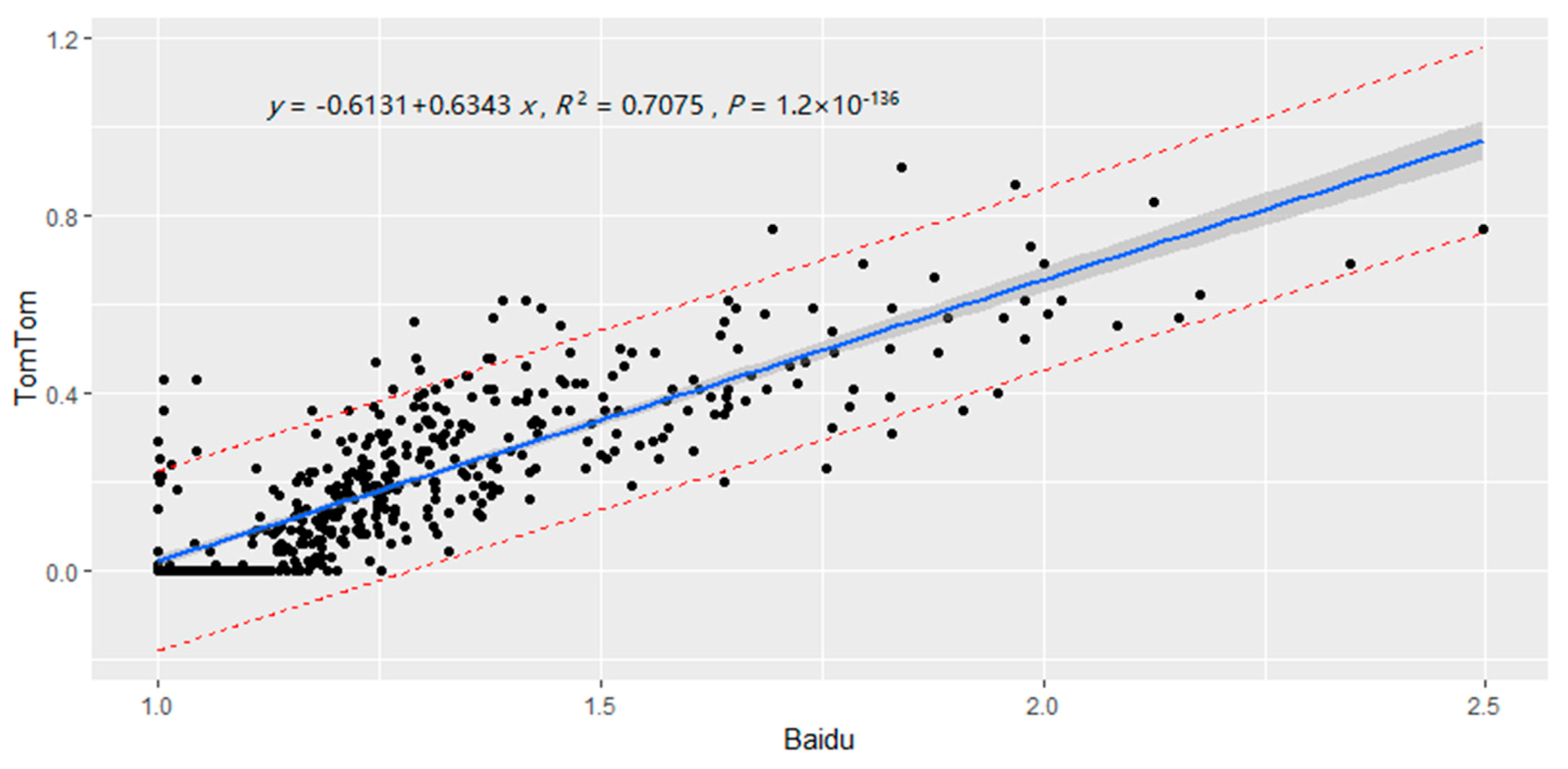
3.1.2. Conversion of Two Traffic Activity Level Indicators

Since the TomTom data set only contains 22 cities in mainland China, in order to apply the research to other Chinese cities, this study converts the two traffic activity level indicators, Baidu Congestion Index (B) and TomTom Congestion Index (X), assuming that The TomTom Congestion Index, predicted by the Baidu Congestion Index, also conforms to the Q(X) relationship to determine the lowest threshold of traffic flow in Chinese cities under free flow (that is, the traffic density is small, and vehicle driving is not affected by other vehicles). Both the TomTom Congestion Index and the Baidu Congestion Index are calculated based on the comparison of actual travel time and free-flow travel time. Therefore, this study assumes that these two indices can be converted.
This study crawled through the TomTom congestion index for the 22 cities in mainland China included in the TomTom congestion index data set with a time granularity of 1 h and the corresponding city’s Baidu congestion index (the original data granularity is 5 min, and the average data granularity is converted to 1 h). A total of 506 observation points are formed to perform simple linear fitting under R 3.4.3 environment (https://cran.r-project.org/bin/windows/base/old/3.4.3/ accessed on 15 January 2021), and the fitting result is shown in Figure 1. Among them, the blue solid line indicates the regression line of the simple linear model. The dark gray area is the 95% confidence interval, which means that the average value of the TomTom congestion index predicted by our linear model specific Baidu congestion index has a 95% probability of being within this area. The area within the red dashed line is the 95% prediction interval, which means that the TomTom congestion index predicted by the Baidu congestion index according to the established linear model has a 95% probability of being within this area at a time, indicating a single predicted value uncertainty.
The fitted two traffic activity level indicators have the following X(B) relationship, where the empirical value of parameter a is 0.6343, and the empirical value of parameter b is −0.6131 (R2 > 0.7, p-value < 0.05).
X = a B + b

3.1.3. Estimation of Road Carbon Emissions Based on Changes in Urban Traffic Levels

This research assumes that the urban vehicle structure and urban road structure will not change significantly within the time frame studied, and the relative change of urban daily road carbon emissions (denoted as E) is proportional to the relative change of Q(X). That is, it is proportional to the relative change in traffic volume. In this way, the establishment of a benchmark for urban road carbon emission levels will enable rapid estimation of China’s urban road carbon emissions and daily monitoring of China’s urban road carbon emissions.
Since this study focuses on the daily fluctuations of carbon emissions on urban roads under the impact of the epidemic, the traffic situation in 2019 is set as the baseline. The study assumes the level of traffic flow during the week from December 16 to December 22, 2019, as the level of traffic flow under normal operating conditions in the city, which is regarded as a benchmark to obtain the relationship between the following day urban road carbon emissions (E) and the relative traffic volume (Q) of the city on a given day, where n is a specific city, and t is a specific date:
E 2020 , n , t = Q 2020 , n , t 7 365 E 2019 , n t = 1 7 Q 2019 ,   n , t
The annual road carbon emissions of each study city are extracted from the high-resolution carbon emissions data of the road transportation department in EDGARv6.0 in 2018. It is assumed that the spatial distribution of urban road carbon emissions has not changed significantly from 2018 to 2019.

3.1.4. Evaluation Method of Road Carbon Emission Control Effect

Use the following formula to evaluate the short-term control effect of the new crown pneumonia epidemic on road carbon emissions:
Δ E p n , t = O b s E n , t S t a E n S t a E n × 100 %
where StaEn is the average daily road carbon emission of each city before the city epidemic; ObsEn,t represents the actual road carbon emission estimated by city n on date t; ∆Epn,t represents the change rate of road carbon emissions of city n on date t, which is used to measure the degree of fluctuation of urban road carbon emissions under the impact of the epidemic.

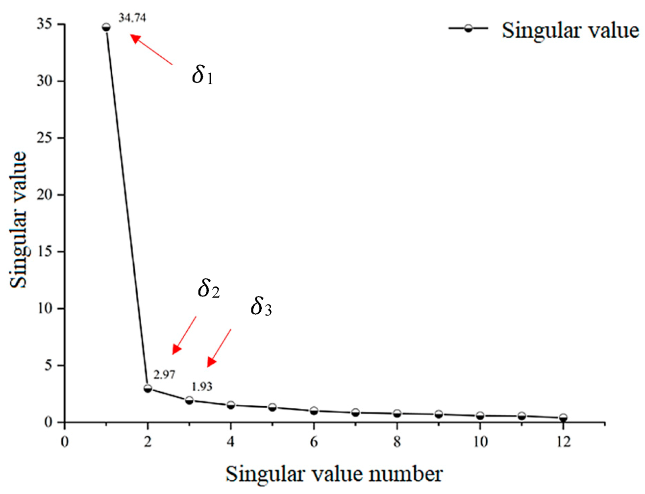
3.2. Spatiotemporal Difference Analysis Method of Road Carbon Emission Changes between Cities Based on Singular Value Decomposition

Under the impact of the epidemic, the changes in road carbon emissions in different cities are unalike and fluctuate over time. In order to more intuitively explain the complex temporal and spatial patterns of urban road carbon emissions under the impact of the epidemic, exploring the similarities and differences in road carbon emissions fluctuations between cities during the considered period, it is necessary to disassemble the original complex model into several simpler spatiotemporal models for characteristic analysis. Singular value decomposition (SVD) is an orthogonal matrix decomposition method that can decompose a matrix into multiple linearly unrelated parts so that researchers can extract the original matrix from multiple simpler matrices. The different characteristics are some of the most basic and important tools of modern numerical analysis. Singular value often corresponds to the important information implicit in the matrix through the rotation, scaling, and projection of the original matrix, and the magnitude of the singular value is positively correlated with the importance of the information. At present, singular value decomposition has been successfully applied in many fields of research dealing with Chinese typefaces [30], resources, and environmental issues [31].
Due to the large differences in the scale of road carbon emissions among cities, the original estimation results of road carbon emissions need to be normalized before performing singular value decomposition. The method is as follows:
E t = E t min ( E t ) max ( E t ) min ( E t )
where Et represents the road carbon emissions of a single city on day t.
Using the normalized raw data, we constructed a spatiotemporal matrix containing the fluctuation characteristics of carbon emissions from the urban road sector from 1 January 2020, to 30 June 2020. There is n (n = 12 in this study) in the date t. The normalized value of urban daily road carbon emissions forms a 1 × n row vector. The normalized value of m-day road carbon emissions can be expressed as a matrix M reflecting the spatiotemporal changes in urban road carbon emissions m × n, namely:
M = ( E 1 , 1 E 1 , n E m , 1 E m , n )
Through singular value decomposition, the normalized space–time matrix of urban road carbon emissions can be expressed as the product of three matrices, which is:
M = U S V T
where M is an m × n matrix, and its rank is r; the left singular matrix U is an m × m matrix, which reflects the time distribution of changes in road carbon emissions; S is a diagonal matrix, and the elements on the diagonal are singular value; the right singular matrix V is an n × n matrix, which reflects the spatial distribution of changes in road carbon emissions. UT and VT are the transposed matrices of U and V, respectively, satisfying UTU = E and VTV = E, and E is the identity matrix. The decomposition is further divided into r matrices with rank 1, namely:
M = U S V T = h = 1 r δ k u k v k T
where uk is the k-th column of U; vk is the k-th column of V; δk is the k-th element singular value of the diagonal matrix S, which is the root of the k-th largest eigenvalue λk of the matrix MTM, in the arrangement δ1 following the maximum value decrease sequentially, and the singular value represents the weight of the decomposed matrix ukvkT in M.
The actual meaning of decomposing the normalized urban road carbon emission spatiotemporal matrix is as follows: M represents the collection of r types of urban road carbon emission change types, uk represents the time distribution of the k-th urban road carbon emission change types, and vkT represents the h-th type. The spatial distribution of urban road carbon emission change types; δk represents the weight of the k-th urban road carbon emission change type. According to the numerical value of the singular value, the most important temporal and spatial characteristics of urban road carbon emissions can be extracted from the complex temporal and spatial changes, and the differences in the fluctuation of carbon emissions from urban roads under the impact of the epidemic can be understood. We input the normalized urban road carbon emission spatiotemporal matrix constructed under the python®3.8.5 environment and perform the singular value decomposition solution and output the result.

3.3. Research Area and Data Sources
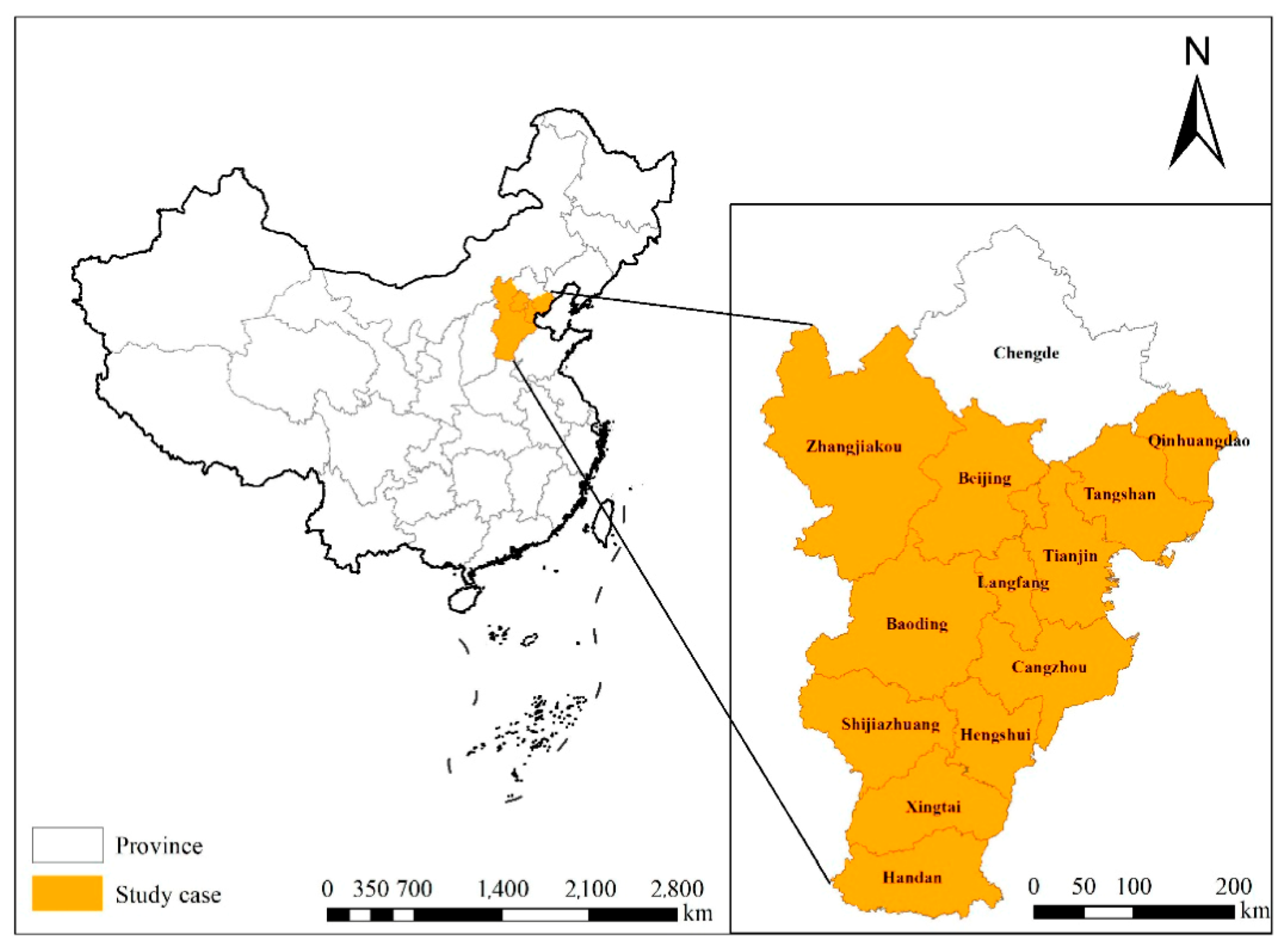
3.3.1. Study Area

The Beijing–Tianjin–Hebei urban agglomeration (JJJ region) is a core area of the North China economy. There are 13 cities in total. As shown in Figure 2, this study is carried out in 12 cities including Beijing, Tianjin, Zhangjiakou, Baoding, Shijiazhuang, Xingtai, Handan, Hengshui, Cangzhou, Langfang, Tangshan, and Qinhuangdao (Chengde not included due to lack of data). From the perspective of the administrative hierarchy of each city, Beijing is the capital, hosting the national political center, cultural center, and international exchange center; Tianjin is a municipality directly under the Central Government, characterized by the northern international shipping core area and by the pioneering area of reform and opening up; Shijiazhuang is the provincial capital; other cities are prefecture-level cities.
The official methods for preventing and controlling of the COVID-19 pandemic in the JJJ region are as follows: The region implemented a Grade I response for major public health emergencies (Public health emergencies response is based on WHO’s Emergency Response Framework, including Resolution EBSS3.R1 on Ebola (2015) and the expansion response to the outbreak of coronavirus disease (COVID-19). According to the impact range and harm degree, public health emergencies response can be divided into four grades: I, II, III, and IV. Grade I is the highest level.) on 24 January 2020, and established a joint prevention and control mechanism in mid-February. The region established close communication and contact in terms of disease prevention in transportation corridors and encouraged the resumption of work and production. After the Spring Festival (1 February), Beijing adopted measures for enterprises to arrange a flexible return to work. The enterprises involved in important national economic activities and necessary for people’s livelihoods, such as those related to epidemic prevention and control, urban operations, and key construction projects, were expected to arrange for employees to return to work normally. In contrast to Beijing’s flexible arrangements, Hebei resumed work and production on 10 February, and Tianjin did the same in mid-February, albeit in batches. Due to the administrative status of Beijing, the coordinated control, and prevention work in the JJJ region, the pandemic become normal (post-lockdown period). Beijing, Tianjin, and Hebei have not adjusted their emergency response levels. At midnight on 30 April, the advisory level for public health emergencies in Beijing, Tianjin, and Hebei was downgraded to Grade II.

3.3.2. Data Sources

The real-time traffic information data used for traffic index conversion were obtained through public platforms. The hourly TomTom traffic congestion index for 22 cities in mainland China was collected from the TomTom official website (https://www.tomtom.com/en_gb/traffic-index/ accessed on 15 January 2021). The real-time Baidu congestion index of the corresponding city was collected from the open platform of Baidu Maps (https://jiaotong.baidu.com/trafficindex/city/curve?cityCode=131&type=minute accessed on 15 January 2021). The annual carbon emissions data of China’s urban road sector were extracted from the road sector carbon emissions (1A3b) in the EDGAR emission database (version v6.0) (https://edgar.jrc.ec.europa.eu/dataset_ghg60 accessed on 15 January 2021). The traffic information of the selected cities from 16 December 2019, to 22 December 2019, and from 1 January 2020, to 30 June 2020, with a time granularity of 1 h, was provided by Baidu Maps Smart Transportation Cooperation. The data on newly added confirmed cases of new coronary pneumonia and Baidu migration data in the research cities were obtained from Harvard Dataverse COVID-19 (https://dataverse.harvard.edu/dataverse/2019ncov accessed on 15 January 2021).

4. Results

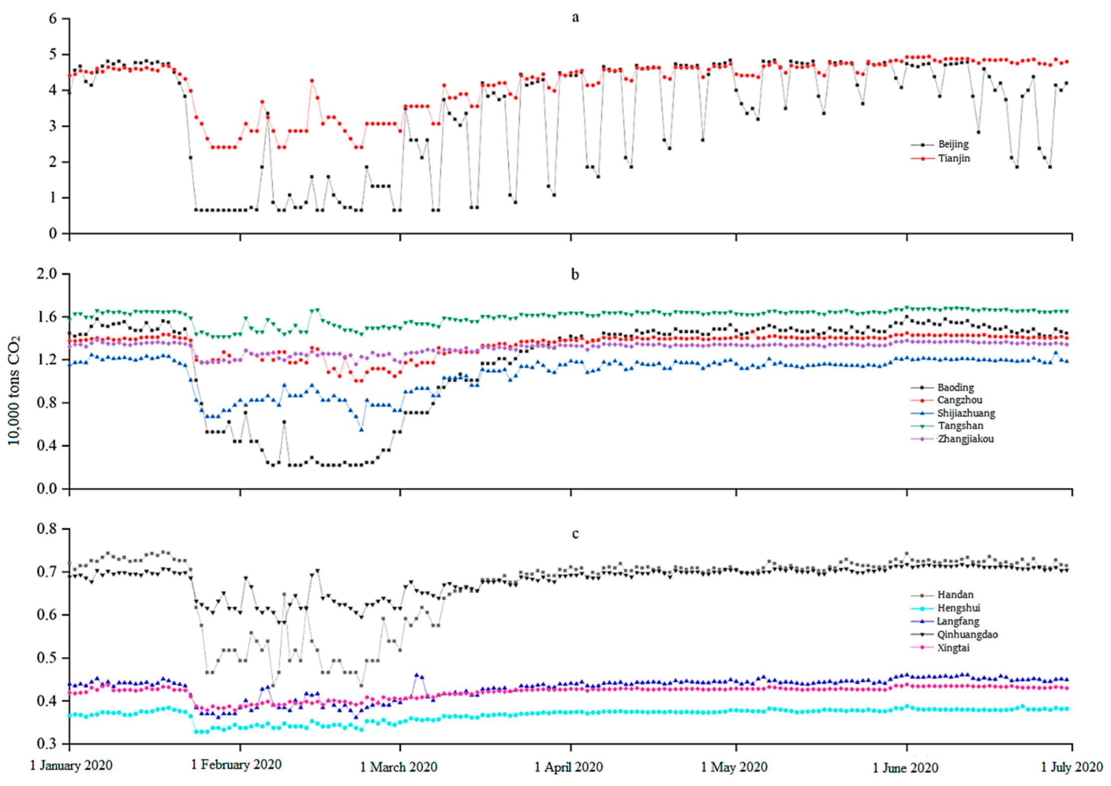
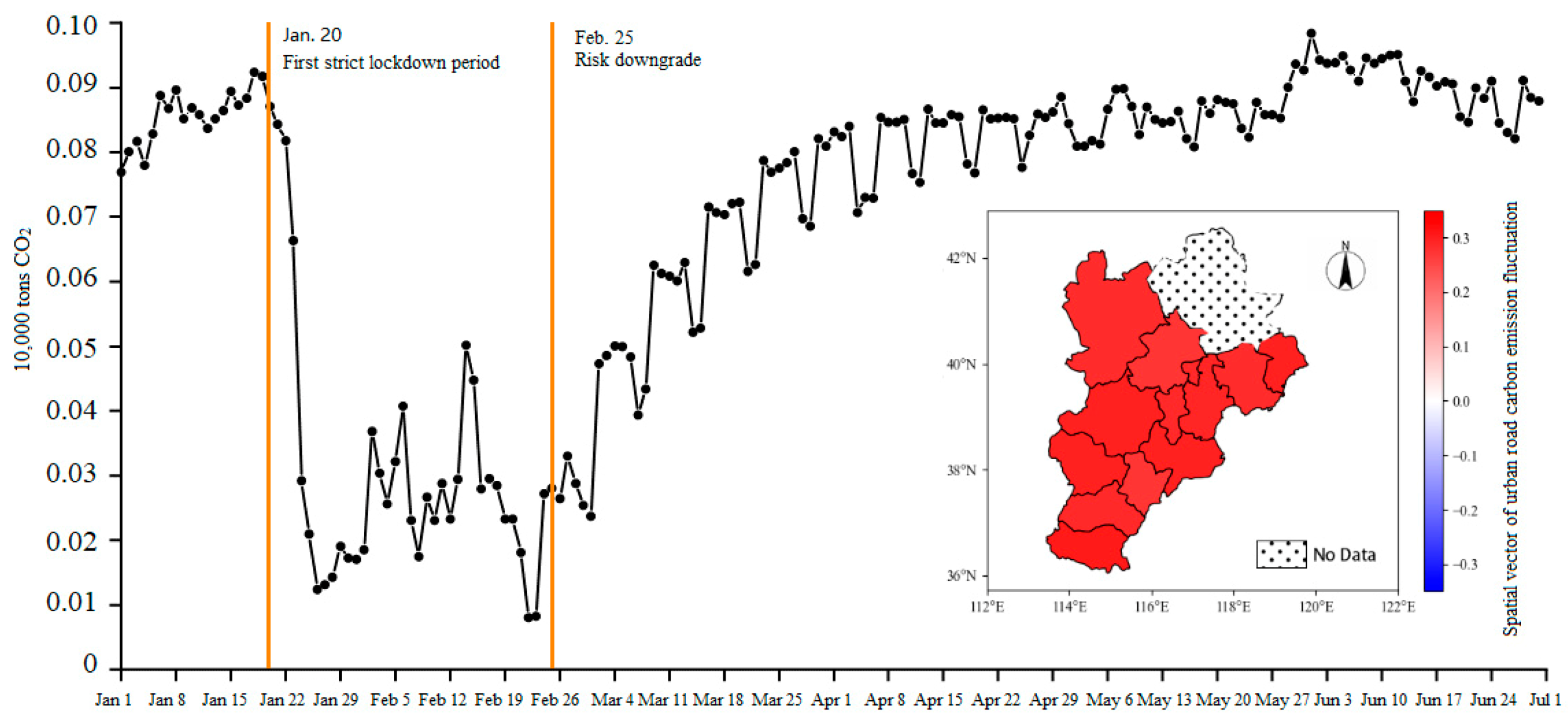
4.1. Estimation of Daily Carbon Emissions from Road Traffic

Comprehensive Equations (1)–(3) estimate the daily road carbon emissions of 12 cities in the JJJ region from 1 January 2020, to 30 June 2020. The results are shown in Figure 3 (see data in Appendix A, Table A1).
Beijing and Tianjin are two of the largest cities in the JJJ region. The average daily road traffic carbon emissions from these cities were similar before the COVID-19 pandemic, amounting to about 45,000 tons, representing the greatest amount among all the cities in the region. Among the considered cities in the region, Beijing’s impact on the pandemic restriction was to respond the earliest and the strongest. On 20 January 2020, Beijing’s daily road traffic carbon emissions began a precipitous decline, dropping to 6500 tons on 24 January, with emission reduction of 86% in just four days. From 24 January to 2 February, Beijing’s road traffic carbon emissions plateaued, after which it remained at a minimum. Beijing’s road traffic carbon emissions remained low throughout February, but there was a significant rebound on 5 and 6 February, with emissions levels of 18,500 and 33,500 tons, respectively. After March, Beijing’s road traffic carbon emissions began to recover and show weekly fluctuations following the resumption of work and production. In the first week of March, the average daily road traffic carbon emissions in Beijing on weekdays was 26,000 tons; in the second week, it rose up to 33,000 tons; in the third week, it rose up to 38,000 tons; in the fourth week, the city’s emissions were close to pre-pandemic levels at 44,000 tons. Carbon emissions on weekdays grew by 16% in March. Following the resumption of work and production in Beijing in March, road traffic carbon emissions rebounded on both weekdays and weekends, with weekday emissions returning to pre-pandemic levels, while weekend emissions remained lower. In April and May, Beijing’s weekday road traffic carbon emissions were relatively stable, at 43,000 to 47,000 tons, while weekend and holiday road traffic carbon emissions remained low but gradually increased. At the end of May, weekend road traffic carbon emissions had recovered to a daily average of 38,500 tons. However, after 11 June, Beijing’s pandemic prevention and control level was, once again, raised due to an outbreak in a Xinfadi farm produce market. In response, the weekdays road traffic carbon emissions dropped slightly from 43,700 to 37,300 tons, and weekend road traffic carbon emissions dropped more significantly from 21,100 to 18,500 tons.
Tianjin is the second largest city in the JJJ region, and its response to the epidemic and the reduction in road carbon emissions was slightly lower than that of Beijing. Its road carbon emissions level was about 45,700 tons before the epidemic “strict lockdown period”. On 24 January, the road carbon emission value in Tianjin was lower than 80% of the average value of road carbon emissions before the COVID-19 emergency, and on 26 January, it was lower than 60% of the average value before the pandemic. After April and May, Tianjin entered the post-lockdown period of recovery and relaxation, and road carbon emissions basically showed a modest increase in working days and weekend fluctuations. The decline was smaller than that showed in March. Road carbon emissions reached an average of 47,500 tons on working days at the end of May, exceeding the average value of the workday before the re-restrictions, indicating that Tianjin had basically returned to recovered economic activities. In June, the emission fluctuation phenomenon had basically disappeared. The daily carbon emissions of roads for the entire month were 48,400 tons, which was higher than Beijing’s carbon emissions during the same period, indicating that Tianjin was developing and resuming work and production rapidly.
Baoding is the city in Hebei Province that responded most dramatically to the epidemic. The average road carbon emissions before the pandemic were about 15,000 tons. After 23 January, the road carbon emissions dropped sharply, and after 26 January, it dropped about the 35% of the emission level registered before the response. After less than 5 days, road carbon emissions continued to fall, reaching a trough of 2200 tons on 7 February, and a decrease of 85%. In February, there was a 24-day low-value period with less than 4000 tons of road carbon emissions, and the daily average of low-value platform areas was about 2600 tons. There was a slight rebound on 9 February, with a value of approximately 6200 tons. After entering March, Baoding’s road carbon emissions entered a stepped upward trend and remained stable. In April and May, the increase was relatively flat. The average daily value of the two months was 14,600 tons. In the first 15 days of June, the average carbon emission increased and exceeded the level before the response, reaching an average of 15,500 tons per day. Perhaps due to the impact of the new outbreak in Beijing, it dropped slightly to 14,600 tons per day after 15 June.
The road carbon emission value of Tangshan City is the highest in Hebei Province, with an average of 16,400 tons per day before the response. In the strict lockdown period, Tangshan City’s response to the epidemic, compared with the road carbon emissions of other cities of the same level in Hebei Province, was not particularly severe, and the lowest level was 87% of that before the response, which was comparable to the response level of Zhangjiakou City. On 27 January, the road carbon emission value of Tangshan City dropped to the lowest value, about 14,200 tons. Throughout February, there were four peaks in road carbon emissions, reaching 15,900 tons, 15,800 tons, 15,200 tons, and 16,700 tons on 2, 6, 11, and 15 February, respectively. After 15 February, road carbon emissions continued to drop to 14,400 tons, about 89% of the level before the response. After entering March, the emission curve slowly declined, but the carbon emission curve suddenly rose during the weekend, with an average growth rate of about 3%. After entering April and May, the daily average level of carbon emissions reached 16,400 tons, returning to the normal level before the epidemic response. Since June, economic development has been progressing, and the daily carbon emission level has reached an average of 16,700 tons, exceeding the level before the response, indicating that after the outbreak of the epidemic, Tangshan City has steadily promoted its economic productivity.

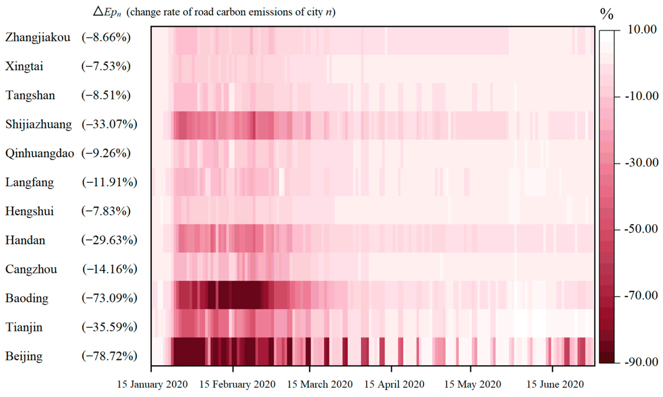
4.2. Policy Effect Analysis for CO2 Reducing Using Short-Term Administrative Controls

From 23 January 2020, to 25 February 2020, the country was subject to a Grade I response for public health emergencies. During this time, the COVID-19 pandemic significantly affected Chinese society in terms of both scale and intensity. Coupled with the massive shutdown of work, production, and schools during the Chinese New Year, there was a significant nationwide decrease in human activity. Since the JJJ region adopted a joint prevention and control mechanism, we believe that the traffic control efforts throughout the 12 cities were similar. In this study, we refer to this period as the “strict lockdown period” and argue that it represents an unprecedented baseline scenario demonstrating the maximum effect for short-term control of road traffic carbon emissions. Moreover, this scenario analysis provides insight of the potential effects of short-term administrative measures addressing the reduction of carbon emissions of the urban road transport sector without changing the existing transportation mix, energy mix, or rates of motor vehicle ownership. It can be seen in Figure 4 that the 12 cities studied showed differences in reduction potentialities and in patterns of fluctuation of the road traffic carbon emissions ( Δ E p n in Equation (4)) during the “strict lockdown period”.
The average rate of change of road traffic carbon emissions in Beijing during the “first strict lockdown period” was −78.72%, which shows that, under short-term administrative control, it has great potential for reducing road traffic carbon emissions. Regarding the speed of the response to the pandemic, Beijing was the most responsive among the 12 cities, with a −53.61% change in road traffic carbon emissions by 23 January. At the same time, due to the special administrative status of Beijing and the severity of the COVID-19 pandemic prevention and control measures, Beijing recovered rapidly in terms of road traffic carbon emissions on weekdays. However, it maintained low emissions levels on the weekends. In June, Beijing’s road traffic carbon emissions once again significantly declined after the outbreak in the Xinfadi farm produce market on 11 June. During this period, the average change rate in road traffic carbon emissions in Beijing was −21.11%, with emissions levels higher than those showed during the “second strict lockdown period”. Meanwhile, road traffic carbon emissions in the nearby 11 cities during the same period were not affected or only slightly affected. This indicates that, during the second strict lockdown period, pandemic prevention and control measures were specifically localized, and the spread of the virus was no longer prevented in the form of undifferentiated, strict prevention and control measures like those employed at the beginning of the pandemic. This shows the impact of China’s cumulative experiences with coronavirus prevention and control and improvements in the scientific nature of prevention and control trough tailored measures.
Road traffic carbon emissions in Baoding also showed great reduction during the “first strict lockdown period”, with an average change rate of −73.09%. In terms of the city’s response to the pandemic, the drop of emissions in Baoding trailed those of Beijing and other cities, which themselves lagged by one to three days. Starting on 23 January, which marked the beginning of the “strict lockdown period”, Baoding’s carbon emissions began by falling −10.48% and continued to drop, reaching −83.83% by 6 February. As the risk posed by the pandemic decreased over time, Baoding’s road traffic carbon emissions showed a gradual increase beginning on 25 February, with the rate of change showing continuous positive values up to 29 May. Given Baoding’s smooth decline in road traffic carbon emissions and gradual recovery following the shock from the pandemic, we speculate that Baoding’s traffic is not sensitive to sudden public events or responses to a policy’s implementation. We also find that response time should be considered when seeking to control road traffic carbon emissions in Baoding through short-term administrative measures such as traffic restrictions and the imposition of tolls.
Handan and Shijiazhuang showed average change rates of −29.63% and −33.07%, respectively, during the “first strict lockdown period”. Before the cities implemented the Grade I responses for public health emergencies, their changes in road traffic carbon emissions ranged from 0–3% compared to their baselines. After June, the rate of change in road traffic carbon emissions remained between −3% and 0%, although main daily activities had largely resumed. This shows that the impact of the COVID-19 pandemic on travel demand in these two cities may be long-lasting and that this slight decline may persist after the pandemic ends.
Cangzhou, Hengshui, Langfang, Qinhuangdao, Tangshan, Xingtai, and Zhangjiakou showed less reduction potential during the “strict lockdown period”, with average change rates of −14.16%, −7.83%, −11.91%, −9.26%, −8.51%, −7.53%, and −8.66%, respectively. This may mean that, in these cities, maintaining basic urban operations accounts for a relatively large volume of road traffic carbon emissions and that further efforts to develop policies to reduce road traffic carbon emissions by regulating travel demand may be ineffective.
The reduction potential for road traffic carbon emissions in Tianjin based on emissions during the “strict lockdown period” was −35.59%. Unlike the other 11 cities, road traffic carbon emissions in Tianjin recovered and increased after the situation stabilized. In June, the rate of change of Tianjin’s road traffic carbon emissions ranged from 3% to 8%, which is a significant increase compared to the pre-pandemic level. This may be due to the need for post-pandemic economic recovery and the increase in logistics demand in Tianjin, given that it is an important port and land transportation hub.

4.3. Analysis of Spatial and Temporal Differences between Cities in Terms of Road Traffic Carbon Emissions

To comprehensively understand the similarities and the differences in road traffic carbon emissions modification between the 12 cities during the COVID-19 pandemic, we use singular value decomposition. This application allows us to decompose and to reduce the spatiotemporal matrix, reflecting the characteristics of road traffic carbon emissions fluctuations from 1 January 2020, to 30 June 2020, identifying the determinants of changes in urban road traffic carbon emissions during the pandemic.
The weights of the normalized urban road traffic carbon emissions matrices obtained using various models are measured by the singular value δ. The larger the singular value, the more original information the pattern contains. Figure 5 is a scree plot of the distribution of singular values from which we can see that the maximum singular value is much larger than the other ones. At the same time, the singular value decreases rapidly, and the change in the fourth and subsequent singular values is extremely small. Therefore, the largest among the first three singular values can be selected, and the corresponding matrices contain 83.68% of the information in the original matrix. The three most important spatial and temporal variation characteristics of urban road traffic carbon emissions can then be extracted.
In this study, three typical spatial and temporal variation characteristics of the road transport sector’s carbon emissions in the cities in the JJJ region during the pandemic were identified based on several singular values and their derived values. In terms of temporal variations under various conditions, the positive and negative temporal unit vectors indicate the fluctuation direction of carbon emissions in the urban road transport sector in the temporal dimension. The absolute value indicates the degree of fluctuation of urban road traffic carbon emissions in the corresponding direction. In terms of spatial variations, the positive and negative values of spatial unit vectors (in which the visualization of spatial variation patterns is divided into warm and cold tones, with warm colors (red) representing positive fluctuations and cold colors (blue) representing negative ones) indicate the fluctuation direction of carbon emissions in the urban road transport sector in the spatial dimension. The absolute value of the spatial unit vectors (shown as the shade of color in the visualization of spatial variation patterns) indicates the degree of fluctuation of urban road traffic carbon emissions in the corresponding direction. Observations of fluctuations in carbon emissions in each type of urban road transport sector can be made by combining the analyses of temporal and spatial vectors. If the temporal unit vector fluctuates significantly in one direction during a specific period and the spatial vector of carbon emissions in an urban road transport sector fluctuates in the same direction significantly, then the carbon emissions of this type of urban road transport sector can be considered to have significantly increased in the corresponding time and space. On the contrary, if the temporal and spatial unit vectors fluctuate in opposite directions, then the carbon emissions of this type of urban road transport sector can be considered to have significantly reduced in the corresponding time and space.

4.3.1. Variation Characteristic I: Overall Trends in the Road Traffic Carbon Emissions

The data of variation characteristic I (singular value: 34.74) in relation to urban road traffic carbon emissions during the pandemic are shown in Figure 6. This model represents the most stable aspect of the spatial and temporal variations in urban road traffic carbon emissions. Compared with other characteristics, this variation characteristic in urban road traffic carbon emissions shows little difference in terms of temporal and spatial distribution. It represents the overall variation characteristic of urban road traffic carbon emissions in the JJJ region during the pandemic. As can be seen from the variation curve for the temporal unit vector while taking 20 January 2020, as the boundary, the temporal flow volatility was relatively stable during the first stage, from 1 January to 20 January. This suggests that urban road traffic carbon emissions levels are relatively stable under normal circumstances in the JJJ region. In the next stage, the temporal unit vector value fell from 0.087 to 0.012, given the impact of the Spring Festival holiday and traffic control measures adopted by various localities in response to the COVID-19 pandemic. This drop of 86.21% indicates that the road traffic carbon emissions in these 12 cities declined significantly during this short period. Secondly, taking 25 February 2020, as the boundary, the temporal unit vector of the overall urban road traffic carbon emissions was lower than usual from 20 January to 25 February, indicating that urban road traffic carbon emissions were lower overall than the pre-pandemic level during this period. After 25 February, the temporal unit vector gradually rebounded and showed an upward fluctuation with a weekly (seven-day) cycle, indicating that the road traffic carbon emission levels in each city gradually recovered as work and production resumed. From May to June, the temporal unit vector was like it was before the pandemic and essentially stable, indicating that the area had entered the normalization phase of the pandemic. In terms of spatial distribution, all cities’ corresponding spatial unit vectors were positive, indicating that the road traffic carbon emissions of all cities in the JJJ region declined rapidly after 20 January and gradually recovered after 25 February, with the overall volatility stabilizing in May and June.

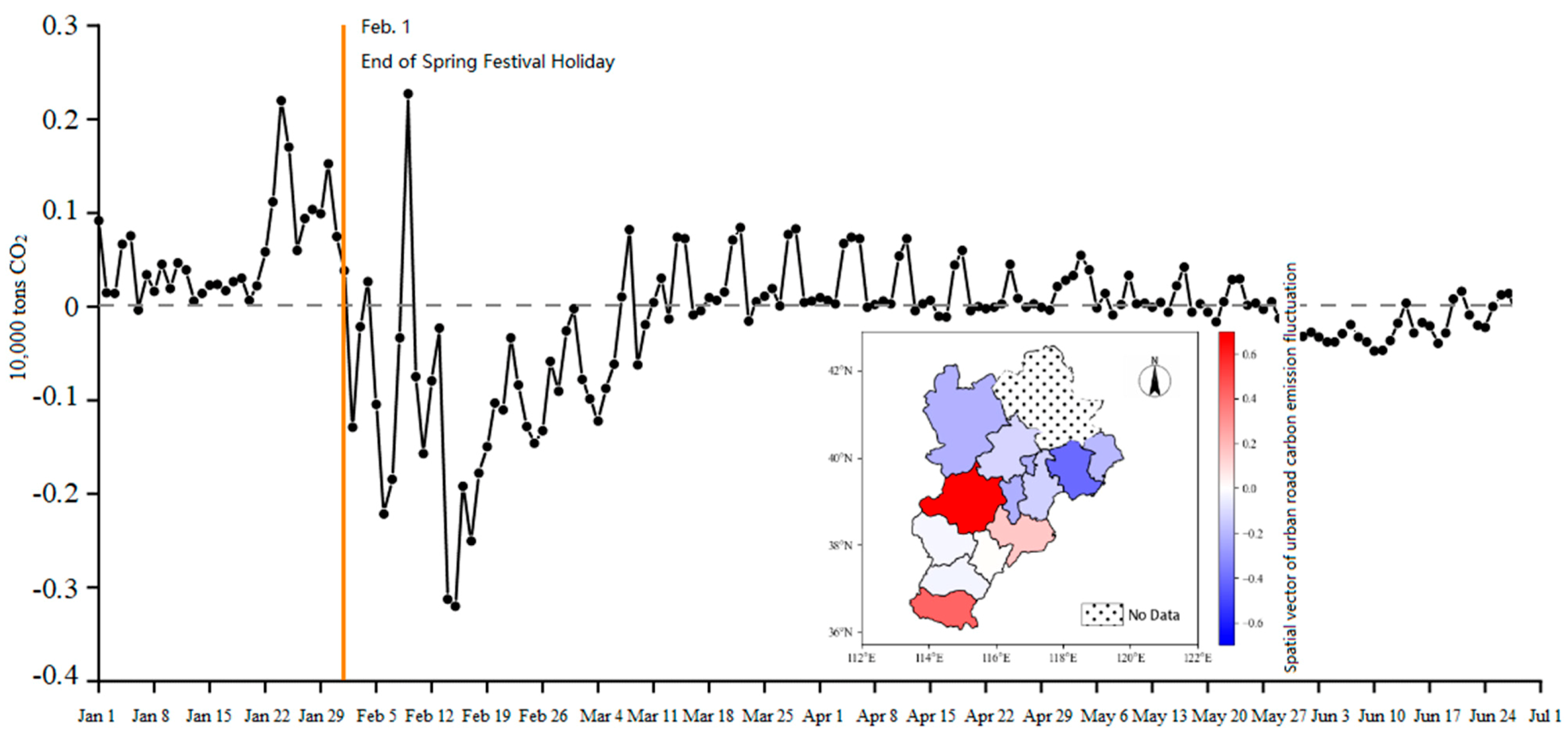
4.3.2. Variation Characteristic II: Differences in Changes of Road Traffic Carbon Emissions in the Cyclical (Weekend and Holiday)

Variation characteristic II (singular value: 2.97) of urban road traffic carbon emissions during the pandemic is shown in Figure 7. The cities that were more strongly affected by prevention and control measures implemented in response to the pandemic can be identified using this characteristic, especially when examining the differences in carbon emissions variations between cities due to differences in the recovery of flexible travel demand, which refers to travel for the purposes of leisure, entertainment, and culture, after the resumption of work and production. In the temporal vector distribution for variation characteristic II of urban road traffic carbon emissions during the pandemic, the focus is placed on the negative fluctuations of weekends and holidays relative to weekdays after 25 February. These negative fluctuations represent the size of the weekend carbon emissions gap relative to weekdays. This characteristic showed evident negative fluctuations with decreasing volatility over five weekends and the Qingming holiday after 25 February. This indicates that there was still a large gap in urban road traffic carbon emissions during this period compared with weekdays. The temporal vector during the Labor Day holiday and the four weekends after 29 April has smaller negative fluctuations, indicating that the urban road traffic carbon emissions gap during this period gradually narrowed compared with weekdays. After the outbreak in the Xinfadi farm produce market in Beijing on 11 June, there were significant negative fluctuations in the temporal flow during weekends and the Dragon Boat Festival, indicating that the outbreak once again led to a significant decrease in urban road traffic carbon emissions compared to the pre-pandemic period. In the spatial vector distribution for variation characteristic II of urban road traffic carbon emissions during the pandemic, the spatial unit vector for Beijing is 0.91, a value much higher than those of other cities, indicating that this characteristic mainly stems from the difference between the fluctuation characteristics of road traffic carbon emissions of Beijing and those of other cities in the JJJ region that arises from differences in the recovery of elastic demand for travel related to leisure, entertainment, and culture represented by weekends and holidays after the resumption of work and production. Beijing had the most severe pandemic prevention and control regime and the strictest control measures of all the cities in the JJJ region. Accordingly, its road traffic carbon emissions characteristics have been significantly different from those of the other cities since the resumption of work and production. This characteristic indicates that the road traffic carbon emissions in Beijing over five weekends and the Qingming holiday after 25 February remained low compared to weekday levels. This low level of emissions gradually recovered after the risk level in the JJJ region declined. Nevertheless, after the outbreak in the Xinfadi market, carbon emissions on weekends and holidays began to decrease significantly. Meanwhile, the spatial unit vectors of Baoding and Tianjin were 0.09 and 0.1, respectively, also showing a subtle expression of this characteristic. As shown in Figure 5, the road traffic carbon emissions of Baoding showed a clear step-wise increase on a weekly basis following the resumption of work and production. The road traffic carbon emissions in Tianjin show a weekly increase, and the emissions levels on weekends are significantly lower than on weekdays. However, the spatial unit vectors of the other cities in the JJJ region are negative, indicating that the flexible travel restrictions on the weekends in these cities have been relaxed to a greater extent than in Beijing and the road traffic carbon emissions gap between weekends and weekdays has narrowed faster.

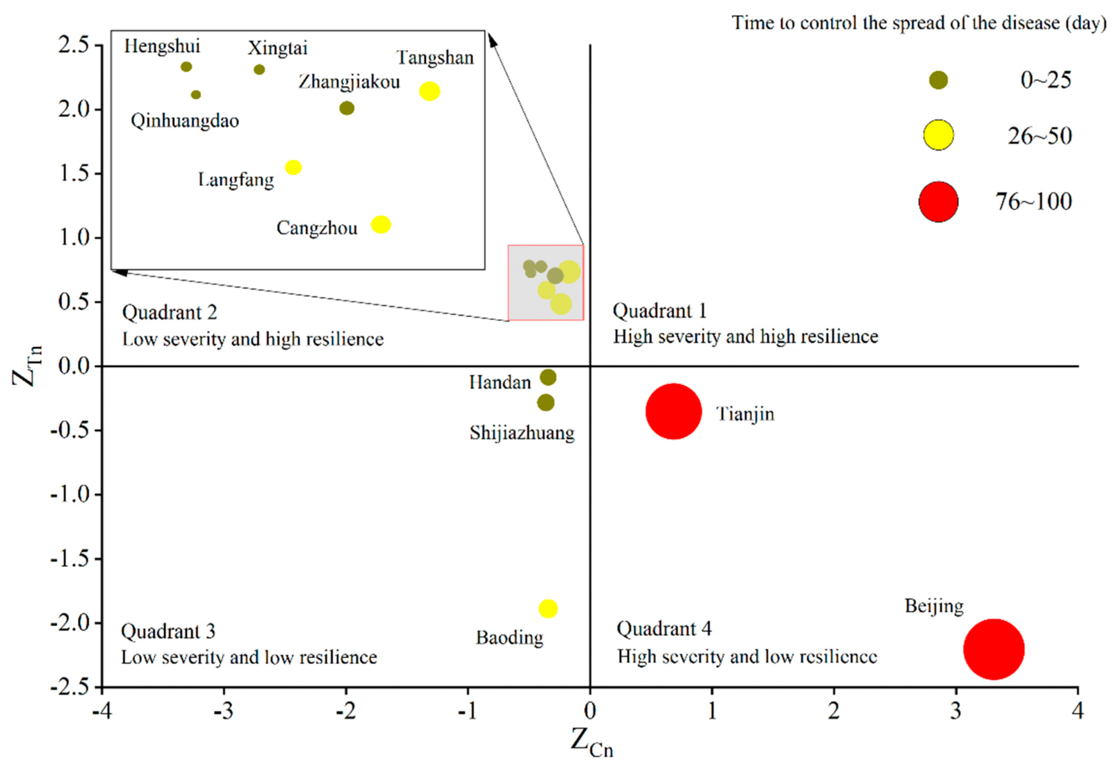
4.3.3. Variation Characteristic III: Differences in Terms of Fluctuations in Road Traffic Carbon Emissions during Major Events Due to the Pandemic

Variation characteristic III (singular value: 1.93) in urban road traffic carbon emissions during the pandemic is shown in Figure 8. In this characteristic, we identified the fluctuations in carbon emissions in various cities before and after the Spring Festival and found that the cities had different responses to the effects of the holiday. When analyzing the temporal vector variation in urban road traffic carbon emissions characteristic III during the pandemic, it can be seen that urban road traffic carbon emissions fluctuated during two periods, 23 January to 1 February and 1 February to 1 March, with 1 February 2020, as the boundary. 1 February 2020, was the last day of the public holiday period of the Spring Festival, so the negative fluctuation in the temporal flow from 1 February to 1 March is interpreted here as the existence of a decreasing trend in road traffic carbon emissions after the Spring Festival relative to the Spring Festival period. There are three types of road traffic carbon emission variations in each city before and after the Spring Festival in terms of spatial distribution. The cities with positive spatial vectors include Baoding and Cangzhou, indicating a trend of a further reduction in road traffic carbon emissions after the Spring Festival in these cities compared to the Spring Festival period. Among them, the absolute value of the spatial unit vector in Baoding was largest, at 0.68, indicating that road traffic carbon emissions in Baoding after the Spring Festival showed a significant downward trend compared to the Spring Festival period. The reason for this variation may be the increase in private car travel in these cities to meet the demand for Spring Festival visits and interactions in the context of the COVID-19 pandemic. The cities with spatial unit vectors close to 0 were Hengshui and Xingtai, indicating that the Spring Festival had little effect on activities in these cities. After removing the effect of the Spring Festival, there was no significant change in the fluctuations in road traffic carbon emissions in these two cities. The cities with negative spatial unit vectors include Beijing, Tianjin, and Tangshan. These cities all showed a more obvious irregular rebound in road traffic carbon emissions after the Spring Festival, indicating that they may have experienced a preliminary resumption of activities after it.
At the same time, it should be noted that the spatiotemporal matrices are extremely complex due to significant differences in the fluctuations in road traffic carbon emissions in the sample cities and a lack of inter-connection between them, which would inevitably lead to a bias when using singular value decomposition for characteristic identification. By comparing the daily road traffic carbon emissions fluctuation curve of each city, we found that deviations in terms of urban road traffic carbon emissions characteristic III during the pandemic were present in the data from Shijiazhuang and Handan. The deviation in Shijiazhuang may have been related to the increase in road traffic carbon emissions in early February and the significant decrease later in the month, while the deviation in Handan may have originated from several significant decreases in road traffic carbon emissions in the city from 1 February to 1 March and the appearance of the lowest values in the time series.

5. Discussion

This study shows that the road traffic carbon emissions of 12 cities in the JJJ region performed distinct fluctuation characteristics and recovery patterns during the pandemic. We believe that this phenomenon reflects, to some extent, these cities’ differing degrees of resilience to the impact of the COVID-19 pandemic in the transportation dimension. The word “resilience” is derived from the Latin word “resilio”, which means “to return to the original state” [27]. The ecologist C.S. Holling first introduced the concept of “ecological resilience” by applying the concept of resilience to systems ecology. Currently, the academic community has essentially reached a consensus on the common characteristics of resilient cities. On the one hand, resilient cities emphasize their ability to buffer themselves from, and adapt to, external shocks and to rebound from adverse, changing influences. On the other hand, they emphasize preventing, preparing for, responding to, and recovering quickly from difficult situations [32]. Most of the thinking and discussions on responding to emergencies and building resilient cities have focused on climate change, environmental disasters, and economic crises, and little focus has been placed on large-scale outbreaks of infectious diseases [33,34,35]. However, the pandemic has posed a significant challenge to cities. In the future, inter-city exchanges will become more prominent, and the activities of people will intersect more frequently as economic development and urbanization advance. Should a major public health emergency such as the COVID-19 pandemic happen again, the chain of responses and amplification effects of urban disasters will inevitably intensify. Therefore, improving cities’ response, adaptability, and recovery capabilities in the face of public health emergencies and other uncertain risks is a real problem that must be addressed when striving to achieve a new type of urbanization.
In this study, since the short-term impact of, and period of recovery from, COVID-19 is closely related to the severity of the pandemic and resilience in each city, we used each city’s cumulative number of confirmed cases (zC, standardized variance) and resilience evaluation index based on road traffic carbon emissions (zT, standardized variance) to divide the cities into four categories: high severity and high resilience, low severity and high resilience, high severity and low resilience, and low severity and low resilience (for detailed calculation methods, see Appendix B).
The first quadrant in Figure 9 represents the cities with high severity and high resilience. The analysis shows that no cities were assigned to the first quadrant, indicating that none of the 12 cities studied could be classified as “high severity and high resilience”. In other words, no city in the JJJ region showed a relatively high level of urban resilience. The second quadrant includes Cangzhou, Hengshui, Langfang, Qinhuangdao, Tangshan, Xingtai, and Zhangjiakou, which showed a low level of exposure risk and relatively quick transmission control. They were thus less affected by the pandemic, with a relatively quick recovery. In addition, we found that this type of city had the smallest economy and population size in the JJJ region and, correspondingly, had a status quo characterized by lower level of population mobility and social aggregation. Therefore, these cities were less affected by the COVID-19 pandemic and showed relatively high levels of urban resilience. The third quadrant includes the cities of Handan, Shijiazhuang, and Baoding, indicating that these cities exhibited relatively weak resilience during the COVID-19 pandemic compared to others in the JJJ region. In terms of risk of exposure, the three cities are linked relatively closely to Wuhan, which may have led to the implementation of relatively strict control measures. In terms of city type, the three cities have populations that are larger than those of the cities in the second quadrant but are lower than those of Beijing and Tianjin, suggesting that cities with larger populations may have weaker resistance and recovery capabilities when attempting to maintain a state of equilibrium in the presence of shocks. At the same time, Shijiazhuang, the provincial capital of Hebei, has a higher level of population inflow, economic development, and population activity than other prefecture-level cities; thus, its control measures have been stricter. As the largest city (by population) bordering Beijing, Baoding was greatly affected by Beijing’s prevention and control measures; correspondingly, its control measures were stricter. Thus, the city has shown weaker resistance and recovery capabilities during the COVID-19 pandemic. Quantitatively speaking, the absolute values of the relative indices of resistance and resilience of Handan and Shijiazhuang are relatively low, indicating that the level of resilience of these two cities is higher than that of Baoding. Beijing and Tianjin, the two mega-cities located in the fourth quadrant (see Figure 9), were the most severely affected by the COVID-19 pandemic. On the one hand, both cities are centrally located and are transportation hubs in the JJJ region, so they have a high level of population inflow, population mobility, and inflow of at-risk populations. Thus, they have a correspondingly higher risk of coronavirus exposure. On the other hand, the two cities have larger populations and higher levels of population density than the others, so the risk of coronavirus transmission has been higher than in some other cities. In terms of their efficiency in controlling the spread of the virus, these two cities took a long time to control its spread, and there were two outbreaks. Given the effect of prevention and control measures, these two cities showed low levels of resistance to and recovery from the pandemic, so they were categorized as cities with “high severity and low resilience”. In addition, when comparing the slope of the line connecting the corresponding points of these two cities to the origin of the virus, we also found that the urban resilience level of Tianjin was slightly higher than that of Beijing. This may be because Beijing, as the center for national administration, had more complex functions and thus less control during the pandemic, making it more difficult for the city to maintain a state of equilibrium.
In summary, the higher a city’s level of urban development and the greater the mobility of a city’s population are, the higher the risk of exposure to major public health emergencies and the more severe their impact will be. At the same time, the larger a city is and the more complex its functions are, the weaker its ability to maintain a state of equilibrium in the face of public emergencies will be. Therefore, large cities should be the focus of such discussions, and it is important to address challenges in preventing and controlling infectious diseases and improve urban resilience.

6. Conclusions and Policy Implication

In order to achieve the goal of carbon neutrality and explore the impact of COVID-19 on urban road carbon emission, we applied a near real-time road carbon emission estimation method for typical Chinese cities in the JJJ region to improve the rapid evaluation of sustainable development. We improved a near real-time road carbon emission estimation method and used singular value decomposition method to this study. As a result, we gathered the daily road carbon emission of 12 cities in the JJJ region under the impact of the epidemic, explored the road carbon reduction effect caused by COVID-19, analyzed the temporal and spatial characteristics of road carbon emission changes among cities, and explored the urban resilience oriented to public events. The results are as follows: (1) In the JJJ region, the carbon reduction effect caused by COVID-19 was significant, but it lasted for a short time. In the three periods—before the epidemic, strict epidemic lockdown and post-lockdown period for prevention and control—the total daily road carbon emissions in the 12 cities were 170,000–190,000 tons, 90,000–110,000 tons, and 160,000–180,000 tons, respectively. (2) Cities in the JJJ region showed different road carbon reduction potential under short-term administrative control. During the “strict lockdown period” (23 January 2020–25 February 2020), the average change rate of road carbon emissions in Beijing was −78.72%, which has great potential for reduction. However, the average change rates of Xingtai and Zhangjiakou were only −7.53% and −8.66 %, respectively. (3) There were spatiotemporal differences in carbon emissions of urban roads in the JJJ region under the impact of the epidemic. With the gradual promotion of re-production, there are great differences between cities on weekends and holidays, and the recovery of road carbon emissions in Beijing on weekends and holidays was far lower than that in other cities. (4) In the face of public emergencies, the larger the city is and the more complex the function of the city is, the more difficult it is for the city to maintain steady state. The resilience indexes of Beijing and Tianjin, which belong to the cities with high severity and low resilience, were −2.2 and −0.35. The resilience indexes of Hengshui, Langfang, and Xingtai, which belong to the cities with low severity and high resilience, were 0.78, 0.59, and 0.78.
Unlike earthquakes, floods, and other disasters that destroy physical spaces, the COVID-19 pandemic destroyed relationships between people. The need to contain the spread of the virus has cut off human contact and connections, a symptom of which is reduced road traffic, which affects the operations of entire cities. Based on this public health emergency, we provide the following considerations and suggestions for building resilient cities:
(1) Strengthen urban safety risk assessments. This study revealed that urban resilience in the context of the COVID-19 pandemic might have been related to factors such as the risk of exposure, severity of the pandemic, and city-level characteristics (i.e., population density, scale of economic activities), which is generally consistent with the results of the existing studies [36,37,38,39,40,41]. Building a resilient city requires further analysis of the basic elements of each city and the current state of public safety measures. This analysis should thus be used as the basis for identifying the various emergencies and risks that each city may need to deal with in the future to formulate appropriate responses.
(2) Encourage the construction of a resilient urban transportation system. Reducing population mobility has been an effective measure for curbing the spread of the coronavirus, but the transportation system is a necessary piece of infrastructure for urban operations. Blocking urban transportation may result in more severe secondary disasters, thereby further impacting social and economic recovery and development. Such an event would also negatively affect the lives of cities’ residents. Therefore, beginning with the temporal dimension, it will be necessary to scientifically research the various stages of a pandemic’s development and develop a model that could, accordingly, be used to protect the transportation system. For example, in the early stage of a pandemic, strict traffic restrictions could be implemented based on spatial isolation needs. When the pandemic is sufficiently contained, the focus could be shifted to balancing disease control with travel recovery. In the middle and late stages of the pandemic, it would be necessary to fully support the recovery of urban mobility. Secondly, beginning with the spatial dimension, the idea of zone-based isolation should be established, with areas divided into severe pandemic areas, key protection areas, and general protection areas based on the density and frequency of confirmed cases. Internal mobility and the operation of public transportation would, likewise, be managed according to zoning classifications.
(3) Strengthen the establishment of information platforms and emergency response systems. With the development of big data, the accessibility of all kinds of basic data on cities, such as information about road congestion, crowd distribution hotspot data, and data on card swiping on public transportation, is increasing. With the support of multiple types of basic data, a professional, real-time emergency response system could be built for tasks such as deploying resources to infected patients and implementing zone-based isolation. Such a system could also allow for rapid decision making and real-time collaboration, which could help prevent incidents that would increase the spread of diseases.

Author Contributions

Conceptualization, G.L.; methodology, G.L. and Z.H.; software, G.L. and Z.H.; validation, G.L. and Z.H.; formal analysis, G.L. and Z.H.; investigation, Y.G., M.W., C.L. and C.C.; resources, G.L. and C.C.; data curation, G.L. and Z.H.; writing—original draft preparation, G.L. and Z.H.; writing—review and editing, G.L., Z.H. and G.V.L.; supervision, G.L.; project administration, G.L.; funding acquisition, G.L. All authors have read and agreed to the published version of the manuscript.

Funding

This work is funded by the National Natural Science Foundation of China (No. 52070021) and the 111 Project (No. B17005).

Institutional Review Board Statement

Not applicable.

Informed Consent Statement

Not applicable.

Data Availability Statement

Not applicable.

Acknowledgments

The comments of reviewers are acknowledged.

Conflicts of Interest

The authors declare no conflict of interest.

Appendix A. Urban Daily Road Carbon Emissions Data

Table A1. Urban daily road carbon emissions data (unit: 10,000 tons) in 2020.
DataBaodingBeijingCangzhouHandanHengshuiLangfangTagnshanTianjinXingtaiZhangjiakouQinhuangdaoShijiazhuang
1 Jan 20201.453.921.380.720.370.441.584.410.421.320.691.15
2 Jan 20201.424.551.380.710.370.431.634.450.421.340.691.17
3 Jan 20201.434.671.380.710.370.441.634.550.421.340.691.18
4 Jan 20201.434.241.390.710.360.431.604.520.421.320.691.17
5 Jan 20201.514.131.400.730.370.441.604.490.431.360.681.24
6 Jan 20201.584.501.400.720.370.451.664.610.431.380.701.22
7 Jan 20201.524.671.390.730.370.441.644.520.431.360.691.20
8 Jan 20201.514.801.400.740.370.441.654.650.441.350.701.22
9 Jan 20201.534.731.390.730.370.431.644.610.421.350.701.21
10 Jan 20201.544.801.390.730.370.441.654.580.421.360.701.21
11 Jan 20201.554.691.400.730.370.441.634.630.431.340.701.22
12 Jan 20201.494.571.390.720.370.441.634.550.431.340.701.21
13 Jan 20201.474.771.390.730.370.441.654.610.421.350.701.20
14 Jan 20201.474.761.410.730.380.441.654.580.431.350.691.21
15 Jan 20201.544.811.410.740.370.441.654.630.431.360.701.23
16 Jan 20201.474.751.410.740.380.441.654.580.431.360.701.21
17 Jan 20201.484.781.410.740.380.441.654.550.431.370.701.22
18 Jan 20201.564.721.440.750.380.451.654.690.431.360.711.24
19 Jan 20201.554.741.430.740.380.451.654.670.431.350.711.23
20 Jan 20201.464.501.410.730.380.441.654.580.431.360.701.19
21 Jan 20201.454.191.400.730.380.441.644.450.431.360.701.17
22 Jan 20201.483.831.400.730.370.431.634.320.421.350.701.15
23 Jan 20201.332.111.380.710.360.411.593.990.411.330.691.01
24 Jan 20201.010.651.200.620.330.381.443.250.391.230.630.82
25 Jan 20200.790.651.170.580.330.371.463.070.381.180.620.73
26 Jan 20200.530.651.170.470.330.371.442.650.381.180.620.67
27 Jan 20200.530.651.200.470.340.371.422.410.391.180.610.67
28 Jan 20200.530.651.200.490.340.361.422.410.381.180.630.67
29 Jan 20200.530.651.270.520.330.371.422.410.381.200.650.73
30 Jan 20200.620.651.240.520.340.371.422.410.391.180.620.73
31 Jan 20200.440.651.200.520.340.371.442.410.381.200.620.78
1 Feb 20200.440.651.200.490.340.381.442.650.391.200.610.82
2 Feb 20200.710.651.290.490.340.401.593.070.391.290.690.78
3 Feb 20200.440.721.260.560.340.381.492.870.391.260.670.82
4 Feb 20200.440.651.240.540.340.381.462.870.391.240.620.82
5 Feb 20200.361.851.200.520.340.431.463.680.391.260.610.82
6 Feb 20200.243.351.260.540.350.431.583.250.401.260.620.86
7 Feb 20200.220.871.200.440.340.391.542.870.391.270.610.82
8 Feb 20200.240.651.270.470.340.381.482.410.391.210.580.78
9 Feb 20200.620.651.270.650.350.381.442.410.391.200.580.96
10 Feb 20200.221.071.170.490.340.381.462.870.401.230.620.86
11 Feb 20200.220.721.170.520.340.401.522.870.391.260.650.86
12 Feb 20200.220.721.200.490.340.381.462.870.391.260.620.86
13 Feb 20200.240.871.170.620.340.421.462.870.401.240.620.90
14 Feb 20200.291.581.310.540.350.411.664.270.391.280.690.96
15 Feb 20200.240.651.300.520.350.421.673.800.401.240.700.90
16 Feb 20200.220.651.260.470.340.381.573.070.391.260.640.82
17 Feb 20200.221.581.080.470.340.401.553.250.401.260.650.82
18 Feb 20200.221.071.120.490.340.391.523.250.401.260.630.86
19 Feb 20200.220.871.050.490.340.381.513.070.401.260.620.82
20 Feb 20200.240.721.220.470.340.391.482.870.401.230.620.82
21 Feb 20200.220.721.080.470.340.381.482.650.391.240.620.73
22 Feb 20200.220.651.000.470.340.361.462.410.391.160.610.67
23 Feb 20200.220.651.000.440.330.381.442.410.391.230.600.54
24 Feb 20200.241.851.080.490.350.381.493.070.411.210.620.82
25 Feb 20200.241.311.120.490.350.391.493.070.401.270.620.78
26 Feb 20200.291.311.120.490.350.401.493.070.391.240.630.78
27 Feb 20200.361.311.120.590.360.391.513.070.411.240.640.78
28 Feb 20200.361.311.080.540.350.391.493.070.401.260.630.78
29 Feb 20200.530.651.050.540.340.401.513.070.411.200.620.73
1 Mar 20200.530.651.080.520.350.401.492.870.401.180.620.73
2 Mar 20200.713.491.170.590.350.411.553.550.411.260.670.90
3 Mar 20200.712.601.200.580.360.411.563.550.411.270.680.90
4 Mar 20200.712.601.150.590.360.461.543.550.411.270.660.93
5 Mar 20200.712.111.170.620.360.451.543.550.411.280.650.93
6 Mar 20200.712.601.170.600.360.411.543.550.411.300.650.93
7 Mar 20200.790.651.170.580.360.401.523.070.411.290.650.86
8 Mar 20200.940.651.310.580.360.411.513.070.411.270.640.86
9 Mar 20200.943.731.260.640.360.421.594.140.421.300.671.03
10 Mar 20201.013.351.270.650.360.421.583.800.421.300.671.03
11 Mar 20201.013.191.290.660.360.421.583.800.421.290.671.03
12 Mar 20201.063.011.270.660.360.421.573.900.421.290.661.03
13 Mar 20201.013.351.270.660.360.421.583.900.421.310.671.05
14 Mar 20201.010.721.270.660.360.411.563.550.421.280.660.96
15 Mar 20201.010.721.270.660.360.411.563.550.421.290.660.96
16 Mar 20201.164.191.330.680.370.431.604.140.421.320.681.11
17 Mar 20201.163.831.330.680.370.431.604.140.421.320.681.09
18 Mar 20201.163.921.330.680.370.431.594.140.421.300.681.09
19 Mar 20201.213.731.350.680.370.431.604.210.421.320.681.09
20 Mar 20201.213.831.350.690.370.431.604.210.421.310.681.11
21 Mar 20201.161.071.320.680.370.421.583.900.421.300.671.01
22 Mar 20201.210.871.340.680.370.421.593.800.431.300.671.05
23 Mar 20201.284.441.370.700.370.431.634.410.421.330.691.14
24 Mar 20201.284.131.370.690.370.431.624.320.431.320.691.14
25 Mar 20201.314.191.380.690.370.431.624.370.431.330.681.13
26 Mar 20201.334.241.360.700.370.441.624.320.431.330.681.18
27 Mar 20201.334.291.380.700.370.441.634.450.431.330.691.15
28 Mar 20201.331.311.360.690.370.431.614.070.431.320.681.09
29 Mar 20201.311.071.360.690.370.431.603.990.431.320.681.08
30 Mar 20201.404.471.380.710.370.441.634.450.431.340.691.15
31 Mar 20201.384.411.380.700.370.441.634.410.431.330.691.15
1 Apr 20201.424.411.390.710.370.441.644.490.431.330.691.19
2 Apr 20201.404.411.380.710.370.441.634.520.431.330.691.18
3 Apr 20201.424.501.400.710.370.441.644.550.431.330.701.18
4 Apr 20201.361.851.360.690.370.431.624.140.421.300.691.08
5 Apr 20201.381.851.380.700.370.431.614.140.431.330.691.09
6 Apr 20201.381.581.390.690.370.431.624.210.431.320.691.11
7 Apr 20201.454.651.410.710.380.441.644.580.431.350.701.18
8 Apr 20201.434.571.400.710.380.441.644.550.431.340.701.16
9 Apr 20201.434.521.410.710.380.441.644.550.431.340.701.19
10 Apr 20201.434.571.390.720.380.441.644.550.431.340.701.16
11 Apr 20201.422.111.390.700.370.441.634.320.431.330.691.11
12 Apr 20201.421.851.390.700.370.441.624.270.431.320.691.12
13 Apr 20201.474.681.410.710.380.441.654.630.431.350.701.18
14 Apr 20201.454.591.400.710.370.441.644.610.431.340.701.16
15 Apr 20201.464.621.400.710.370.441.644.610.431.340.701.15
16 Apr 20201.474.621.410.710.370.441.664.650.431.340.701.15
17 Apr 20201.454.621.400.710.370.441.654.630.431.350.701.17
18 Apr 20201.432.601.400.700.370.441.634.370.431.330.701.12
19 Apr 20201.432.371.400.700.380.441.634.320.431.320.691.12
20 Apr 20201.484.731.400.710.370.451.654.650.431.340.701.18
21 Apr 20201.464.681.400.710.370.441.654.630.431.330.701.17
22 Apr 20201.464.681.400.710.370.451.644.630.431.330.701.17
23 Apr 20201.464.651.400.710.370.441.644.630.431.340.701.17
24 Apr 20201.464.681.400.710.370.441.644.630.431.330.701.17
25 Apr 20201.432.601.390.700.370.441.634.370.431.330.701.12
26 Apr 20201.434.441.390.700.370.441.634.580.431.330.701.15
27 Apr 20201.484.731.400.710.370.441.644.670.431.340.701.17
28 Apr 20201.484.721.400.710.370.441.644.650.431.340.701.16
29 Apr 20201.484.761.400.710.380.441.644.670.431.340.711.19
30 Apr 20201.524.831.400.710.380.451.654.740.431.340.701.20
1 May 20201.474.001.410.710.380.441.634.450.431.340.701.16
2 May 20201.433.611.400.700.380.441.634.410.431.330.701.12
3 May 20201.453.351.400.700.380.441.624.410.431.340.701.12
4 May 20201.463.491.460.700.380.441.624.410.431.330.701.15
5 May 20201.483.191.400.700.380.451.634.370.431.330.701.13
6 May 20201.494.801.400.710.380.461.634.670.431.340.701.15
7 May 20201.524.791.420.720.380.451.654.710.431.340.701.21
8 May 20201.504.831.420.720.380.451.664.790.431.340.711.16
9 May 20201.474.621.410.710.380.441.644.650.431.340.711.17
10 May 20201.473.491.410.710.380.441.634.490.431.330.701.15
11 May 20201.494.801.410.710.380.441.654.690.431.340.711.15
12 May 20201.474.771.400.710.370.441.654.650.431.330.701.14
13 May 20201.464.751.400.710.370.441.644.650.431.340.701.13
14 May 20201.464.731.400.710.380.441.654.670.431.330.701.15
15 May 20201.474.801.410.710.380.441.654.710.431.340.701.15
16 May 20201.433.831.410.700.380.441.634.490.431.330.701.15
17 May 20201.453.351.400.700.380.441.634.410.431.320.701.16
18 May 20201.494.781.410.710.380.441.654.770.431.340.711.16
19 May 20201.474.761.400.710.380.441.644.710.431.340.701.15
20 May 20201.474.781.410.720.380.441.654.750.431.350.711.15
21 May 20201.454.751.400.730.380.451.664.770.431.340.711.15
22 May 20201.504.761.400.720.380.451.654.740.431.350.701.15
23 May 20201.464.131.400.720.380.441.634.490.431.340.701.15
24 May 20201.453.611.400.710.380.451.634.450.431.330.701.14
25 May 20201.504.751.410.710.380.451.644.800.431.340.701.15
26 May 20201.474.711.410.710.380.441.654.710.431.330.701.15
27 May 20201.464.731.400.710.380.441.644.720.431.330.711.14
28 May 20201.464.771.400.710.380.441.644.710.431.330.701.15
29 May 20201.514.801.420.720.380.451.664.820.431.350.711.17
30 May 20201.544.331.430.730.380.461.674.840.441.370.711.21
31 May 20201.544.071.430.720.380.461.674.810.431.370.711.20
1 Jun 20201.604.741.450.740.390.461.694.930.441.380.721.22
2 Jun 20201.564.681.430.730.380.461.684.920.431.370.711.20
3 Jun 20201.544.651.430.720.380.451.674.930.431.370.711.20
4 Jun 20201.544.721.430.720.380.451.674.930.431.370.721.21
5 Jun 20201.564.741.430.730.380.461.684.950.431.370.721.21
6 Jun 20201.534.371.430.720.380.451.674.840.431.370.711.21
7 Jun 20201.523.831.430.720.380.461.664.800.431.370.711.20
8 Jun 20201.584.701.430.730.380.461.684.880.431.370.711.21
9 Jun 20201.554.731.430.720.380.451.684.890.431.370.711.20
10 Jun 20201.544.741.430.720.380.461.684.870.431.370.711.20
11 Jun 20201.544.771.430.730.380.461.684.890.431.370.721.21
12 Jun 20201.564.791.430.730.380.461.684.880.441.370.711.21
13 Jun 20201.523.831.430.720.380.451.664.830.431.370.721.21
14 Jun 20201.502.821.430.720.380.451.664.770.431.360.711.20
15 Jun 20201.524.591.430.720.380.451.674.860.431.360.711.20
16 Jun 20201.504.371.420.740.380.451.674.850.441.360.711.20
17 Jun 20201.484.001.420.730.380.451.674.840.431.360.711.19
18 Jun 20201.484.191.410.720.380.461.674.860.431.360.711.20
19 Jun 20201.503.731.420.720.380.451.674.860.431.370.711.20
20 Jun 20201.462.111.420.720.380.451.664.780.431.360.711.19
21 Jun 20201.451.851.410.720.380.451.654.750.431.350.711.18
22 Jun 20201.473.831.410.730.390.451.664.830.431.360.711.19
23 Jun 20201.464.001.400.720.380.451.664.840.431.350.711.19
24 Jun 20201.484.371.410.730.380.451.664.860.431.360.711.21
25 Jun 20201.432.371.410.710.380.451.654.750.431.350.711.19
26 Jun 20201.422.111.400.710.380.441.654.740.431.350.701.17
27 Jun 20201.421.851.400.710.380.441.654.710.431.350.711.17
28 Jun 20201.484.131.410.730.380.451.654.860.431.360.711.26
29 Jun 20201.464.001.420.720.380.451.654.770.431.350.701.20
30 Jun 20201.454.191.400.710.380.451.654.800.431.340.701.18

Appendix B. UrbanR and Severity Evaluation Model

In this study, since the short-term impact of, and period of recovery from, the COVID-19 is closely related to the severity of the pandemic and resilience in each city, we used city’s cumulative number of confirmed cases (zC, standardized variance) and resilience evaluation index based on road traffic carbon emissions (zT, standardized variance) to divide the cities.
First, we use the carbon emissions of each city’s roads to construct a Relative Recovery Index (RRI) as an indicator to measure the relative recovery of the city:
R R I n , t = O b s E n , t S t a E n
where, RRIn,t is the recovery index of city n at time t; same as Equation (4), ObsEn,t is the actual value of road carbon emissions of city n at time t; StaEn is the benchmark road carbon emissions of each city before the epidemic.
In order to comprehensively evaluate the resilience of the cities in the early stage of the epidemic, we focused on analyzing the period from 20 January (JJJ emergency response level was set in Grade I) to 30 April (after that, the emergency response level was downgraded to Grade II). 8 evaluation sub-periods are selected: Phase 1 is from 20 January to 26 January; Phase 2 is from 27 January to 2 February; Phase 3 is from 10 February to 16 February; Phase 4 is from 24 February to 1 March; Phase 5 is from 9 March to 15 March; Phase 6 is from 23 March to 29 March; Phase 7 is from 6 April to 12 April; Phase 8 is from 20 April to 30 April. Taking the weekly RRIs of each sub-period as the evaluation index, Phases 1 and 2 are used to measure the resilience of cities when the epidemic suddenly breaks out; Phases 3–8 are used to measure the resilience of cities under the continuous impact of the epidemic. Information entropy is calculated to determine the index weights according to the amount of information provided by the observation value. This study introduces the information entropy method to construct an evaluation model to evaluate the resilience of each city under the impact of the epidemic. The steps are as follows:
(1)
Construct evaluation index: Xnj is the j-th index value of city n.
(2)
Calculate the proportion of the j-th index of the n-th city in the city:
P n j = X n j n = 1 y X n j
(3)
Calculate the information entropy of the j-th index:
S j = k n = 1 y P n j l n ( P n j )
where k = 1/ln(y) > 0, satisfying Sj ≥ 0.
(4)
Calculate the information utility of the j-th index:
D j = 1 S j
(5)
Calculate the weight of index:
W j = D j j = 1 m D j
(6)
Calculate the comprehensive score of each city’s resilience:
T n = j ( W j x n j )
According to Equations (A2)–(A6), we calculated the comprehensive score index T for resilience evaluation of each city. After that, we standardized index T and urban cumulative COVID-19 cases C (the count ends 30 April 2020) based on Z-score standardization, as follows:
z T n = T n T n ¯ δ T
z C n = C n C n ¯ δ C
where, zTn is the standardized variance of the comprehensive score of the RRIs in city n; zCn is the standardized variance of the cumulative number of confirmed cases in city n. Z-score standardization is based on the mean ( T n ¯ or C n ¯ ) and standard deviation ( δ T or δ C ) of the original data, and the z-score obtained conforms to the standard normal distribution. According to the n-th city’s cumulative number of confirmed cases (zCn, standardized variance) and resilience evaluation index based on road traffic carbon emissions (zTn, standardized variance), the relative positives of the cities’ severity and resilience can be obtained (see Figure 9).

References

  1. Zhang, L.L.; Long, R.Y.; Chen, H.; Geng, J.C. A review of China’s road traffic carbon emissions. J. Clean. Prod. 2019, 207, 569–581. [Google Scholar] [CrossRef]
  2. Bueno, G. Analysis of scenarios for the reduction of energy consumption and GHG emissions in transport in the Basque Country. Renew. Sustain. Energy Rev. 2012, 16, 1988–1998. [Google Scholar] [CrossRef]
  3. Xu, B.; Lin, B.Q. Investigating the differences in CO2 emissions in the transport sector across Chinese provinces: Evidence from a quantile regression model. J. Clean. Prod. 2018, 175, 109–122. [Google Scholar] [CrossRef]
  4. Cai, B.F.; Feng, X.Z.; Chen, X.M. Carbon Dioxide Emissions from Transport and Low-Carbon Development; Chemical Industry Press: Beijing, China, 2012. [Google Scholar]
  5. Li, F.; Cai, B.; Ye, Z.; Wang, Z.; Zhang, W.; Zhou, P.; Chen, J. Changing patterns and determinants of transportation carbon emissions in Chinese cities. Energy 2019, 174, 562–575. [Google Scholar] [CrossRef]
  6. IEA. CO2 Emissions from Fuel Combustion: Overview; IEA: Paris, France, 2020. [Google Scholar]
  7. de Oliveira Neto, G.C.; Correia JM, F.; Silva, P.C.; Sanches AG, O.; Lucato, W.C. Cleaner Production in the textile industry and its relationship to sustainable development goals. J. Clean. Prod. 2019, 228, 1514–1525. [Google Scholar] [CrossRef]
  8. Baltazar, J.; Reis, J.; Amorim, M. Sustainable economies: Using a macro-economic model to predict how the default rate is affected under economic stress scenarios. Sustain. Futures 2020, 2, 100011. [Google Scholar] [CrossRef]
  9. Ibn-Mohammed, T.; Mustapha, K.B.; Godsell, J.; Adamu, Z.; Babatunde, K.A.; Akintade, D.D.; Acquaye, A.; Fujii, H.; Ndiaye, M.M.; Yamoah, F.A.; et al. A critical analysis of the impacts of COVID-19 on the global economy and ecosystems and opportunities for circular economy strategies. Resour. Conserve. Recycl. 2021, 164, 105169. [Google Scholar] [CrossRef]
  10. IEA. Global Energy Review; IEA: Paris, France, 2021. [Google Scholar]
  11. Forster, P.M.; Forster, H.I.; Evans, M.J.; Gidden, M.J.; Jones, C.D.; Keller, C.A.; Lamboll, R.D.; Quéré, C.L.; Rogelj, J.; Rosen, D.; et al. Current and future global climate impacts resulting from COVID-19. Nat. Clim. Chang. 2020, 10, 913–919. [Google Scholar] [CrossRef]
  12. Alemdar, K.D.; Kaya, Ö.; Canale, A.; Çodur, M.Y.; Campisi, T. Evaluation of Air Quality Index by Spatial Analysis Depending on Vehicle Traffic during the COVID-19 Outbreak in Turkey. Energies 2021, 14, 5729. [Google Scholar] [CrossRef]
  13. Aletta, F.; Brinchi, S.; Carrese, S.; Gemma, A.; Guattari, C.; Mannini, L.; Patella, S.M. Analysing urban traffic volumes and mapping noise emissions in Rome (Italy) in the context of containment measures for the COVID-19 disease. Noise Mapp. 2020, 7, 114–122. [Google Scholar] [CrossRef]
  14. Hu, S.G.; Wang, R.H.; Wang, X.X.; Liu, Y.Y. Modeling of Travel Mode Choice Behavior of Residents in Different Stages of the COVID-19 Epidemic. J. Guangdong Univ. Technol. 2021, 38, 32–38. [Google Scholar]
  15. Wu, L.W. GPS Based Travel Characteristics of Private Passenger Cars in Beijing. Ph.D. Thesis, Tsinghua University, Beijing, China, 2013. [Google Scholar]
  16. Zhang, X.Y.; Yang, X.M.; Yan, Y. Statistical Estimation Method for Energy Consumption and Carbon Emissions by Urban Transport. China Soft Sci. 2014, 142–150. [Google Scholar]
  17. Schipper, L.; Marie-Lilliu, C.; Gorham, R. Flexing the Link between Transport and Greenhouse Gas Emissions: A Path for the World Bank; IEA: Paris, France, 2000. [Google Scholar]
  18. Puliafito, S.E.; Allende, D.; Pinto, S.; Castesana, P. High resolution inventory of GHG emissions of the road transport sector in Argentina. Atmos. Environ. 2015, 101, 303–311. [Google Scholar] [CrossRef]
  19. The United States Environmental Protection Agency (USEPA). User’s Guide to MOBILE6.1 and MOBILE6.2: Mobile Source Emission Factor Model. Office of Transportation and Air Quality; US Environmental Protection Agency: Washington, DC, USA, 2002.
  20. European Environment Agency (EEA). COPERT III Computer Programme to Calculate Emissions from Road Transport–Methodology and Emissions Factors (Version 2.1); Ntziachristos, L., Samaras, Z., Eggleston, S., Gorissen, N., Hassel, D., Hickman, A.-J., Joumard, R., Rijkeboer, R., White, L., Zierock, K.-H., Eds.; Technical Report No. 49; European Environment Agency: Copenhagen, Denmark, 2000. [Google Scholar]
  21. CARB. EMFAC2014 User’s Guide; California Air Quality Research Board CARB: Sacramento, CA, USA, 2014.
  22. Chang, X.M.; Chen, B.Y.; Li, Q.Q.; Cui, X.H.; Tang, L.I.; Liu, C. Estimating real-time traffic carbon dioxide emissions based on intelligent transportation system technologies. IEEE Trans. Intell. Transport. Syst. 2013, 14, 469–479. [Google Scholar] [CrossRef]
  23. Zheng, B.; Geng, G.; Ciais, P.; Davis, S.J.; Martin, R.V.; Meng, J.; Wu, N.; Chevallier, F.; Broquet, G.; Boersma, F.; et al. Satellite-based estimates of decline and rebound in China’s CO2 emissions during COVID-19 pandemic. Sci. Adv. 2020, 6, eabd4998. [Google Scholar] [CrossRef] [PubMed]
  24. Wang, R.; Xiong, Y.; Xing, X.; Yang, R.; Li, J.; Wang, Y.; Cao, J.; Balkanski, Y.; Penuelas, J.; Ciais, P.; et al. Daily CO2 Emission Reduction Indicates the Control of Activities to Contain COVID-19 in China. Innovation 2020, 1, 100062. [Google Scholar] [CrossRef]
  25. Han, P.; Cai, Q.; Oda, T.; Zeng, N.; Shan, Y.; Lin, X.; Liu, D. Assessing the recent impact of COVID-19 on carbon emissions from China using domestic economic data. Sci. Total Environ. 2021, 750, 141688. [Google Scholar] [CrossRef]
  26. Shan, Y.L.; Guan, D.B.; Hubacek, K.; Zheng, B.; Davis, S.J.; Jia, L.C.; Liu, J.H.; Liu, Z.; Fromer, N.; Mi, Z.F.; et al. City-level climate change mitigation in China. Sci. Adv. 2018, 4, eaaq0390. [Google Scholar] [CrossRef] [Green Version]
  27. Shao, Y.W.; Xu, J. Understanding Urban Resilience: A Conceptual Analysis Based on Integrated International Literature Review. Urban Plann. Int. 2015, 30, 48–54. [Google Scholar]
  28. Le Quéré, C.; Jackson, R.B.; Jones, M.W.; Smith, A.J.P.; Abernethy, S.; Andrew, R.M.; De-Gol, A.J.; Willis, D.R.; Shan, Y.; Canadell, J.G.; et al. Temporary reduction in daily global CO2 emissions during the COVID-19 forced confinement. Nat. Clim. Chang. 2020, 10, 647–653. [Google Scholar] [CrossRef]
  29. Liu, Z.; Ciais, P.; Deng, Z.; Lei, R.; Davis, S.J.; Feng, S.; Zheng, B.; Cui, D.; Dou, X.; Zhu, B.; et al. Near-real-time monitoring of global CO2 emissions reveals the effects of the COVID-19 pandemic. Nat. Commun. 2020, 11, 5172. [Google Scholar] [CrossRef]
  30. Zhang, Y.; Xie, Y.; Hong, C.; Qu, Y.Y.; Li, R.; Zhang, J.S.; Li, C.H. Esthetic preference mining of Chinese typefaces using multiview cluster analysis. Sci. Sin. Inform. 2021, 51, 383–398. [Google Scholar] [CrossRef]
  31. Wei, Y.N.; Li, X.G.; Li, F. Spatial distribution characteristics and influencing factors of wet and dry of runoff in upper reaches of the Yellow River. Water Resour. Prot. 2021, 37, 103–113. [Google Scholar]
  32. Bing, Q.L. Build resilient cities to cope with major public health emergencies. Urban Rural Dev. 2020, 14, 6–10. [Google Scholar]
  33. Shamsuddin, S. Resilience resistance: The challenges and implications of urban resilience implementation. Cities 2020, 103, 8. [Google Scholar] [CrossRef] [PubMed]
  34. Zou, L.; Lam, N.S.N.; Cai, H.; Qiang, Y. Mining Twitter Data for Improved Understanding of Disaster Resilience. Annals 2018, 108, 1–20. [Google Scholar] [CrossRef]
  35. Godschalk, D.R. Urban Hazard Mitigation: Creating Resilient Cities. Urban Plann. Int. 2015, 30, 22–29. [Google Scholar] [CrossRef]
  36. Chen, J.; Guo, X.; Pan, H.; Zhong, S. What determines city’s resilience against epidemic outbreak: Evidence from China’s COVID-19 experience. Sustain. Cities Soc. 2021, 70, 102892. [Google Scholar] [CrossRef] [PubMed]
  37. Connolly, C.; Keil, R.; Ali, S.H. Extended urbanisation and the spatialities of infectious disease: Demographic change, infrastructure and governance. Urban Stud. 2021, 58, 245–263. [Google Scholar] [CrossRef]
  38. Lai, K.Y.; Webster, C.; Kumari, S.; Sarkar, C. The nature of cities and the COVID-19 pandemic. Curr. Opin. Environ. Sustain. 2020, 46, 27–31. [Google Scholar] [CrossRef]
  39. Tong, J.; Ma, Y.; Liu, H.M. The short-term impact of COVID-19 epidemic on the migration of Chinese urban population and the evaluation of Chinese urban resilience. Acta Geogr. Sin. 2020, 75, 2505–2520. [Google Scholar]
  40. Dalziel, B.D.; Pourbohloul, B.; Ellner, S.P. Human mobility patterns predict divergent epidemic dynamics among cities. Proc. R. Soc. B-Biol. Sci. 2013, 280, 20130763. [Google Scholar] [CrossRef] [PubMed]
  41. Prashar, S.; Shaw, R.; Takeuchi, Y. Assessing the resilience of Delhi to climate-related disasters: A comprehensive approach. Nat. Hazards 2012, 64, 1609–1624. [Google Scholar] [CrossRef]
Figure 1. Baidu Congestion Index vs. TomTom Congestion Index. (The solid blue line is the regression line. The gray area is the confidence interval. The red dashed line is the prediction interval).
Sustainability 14 00385 g001
Figure 2. Research Area.
Sustainability 14 00385 g002
Figure 3. Daily road carbon emissions in 12 cities from 1 January to 30 June 2020 ((a). Beijing and Tianjin; (b). Baoding, Cangzhou, Shijiazhuang, Tangshan and Zhangjiakou; (c). Handan, Hengshui, Langfang, Qinhuangdao and Xingtai).
Sustainability 14 00385 g003
Figure 4. Change rate of urban road carbon emissions from 15 January to 30 June 2020.
Sustainability 14 00385 g004
Figure 5. The distribution of singular values of the spatiotemporal matrix of normalized urban road carbon emissions (δ is the singular value).
Sustainability 14 00385 g005
Figure 6. Spatiotemporal distribution of changes in urban road carbon emissions under the impact of the epidemic (variation characteristic I: singular value δ 1 = 34.74).
Sustainability 14 00385 g006
Figure 7. Spatiotemporal distribution of changes in urban road carbon emissions under the impact of the epidemic (variation characteristic II: singular value δ 2 = 2.97).
Sustainability 14 00385 g007
Figure 8. Spatiotemporal distribution of changes in urban road carbon emissions under the impact of the epidemic (variation characteristic III: singular value δ 3 = 1.93).
Sustainability 14 00385 g008
Figure 9. Bubble chart of urban resilience index and the severity of the pandemic (zCn is the standardized variance of the cumulative number of confirmed cases in city n; zTn is the standardized variance of the resilience evaluation index in city n).
Sustainability 14 00385 g009
Publisher’s Note: MDPI stays neutral with regard to jurisdictional claims in published maps and institutional affiliations.

