1. Introduction
Improving sustainability on the production and consumption sides of product life cycles has proven to be critical in reducing the carbon footprint and combating global warming [
1]. For this reason, one of the United Nations Sustainable Development Goals (i.e., Goal #12) explicitly addresses the problems associated with unsustainable production and consumption (
https://www.un.org/sustainabledevelopment/sustainable-development-goals/ (accessed on 22 December 2021). Many manufacturers shift production to low-cost and distant countries to benefit from low production costs, but the long production and shipping lead times between production and the market bases contribute to significant amounts of excess inventory [
2] that risk going to waste in retail stores without ever reaching consumers. The cost of excess inventory in the retail industry was estimated to be USD 471 billion in 2014 [
3]. In other words, the Earth’s resources to a value of USD 471 billion are wasted in producing goods that are never sold, and hence never used, by any consumer.
Let us consider the apparel industry, which is responsible for 8–10% of global carbon emissions [
4]. The industry is dominated by strong brands that outsource production to contract manufacturers in offshore countries that rely on coal-fueled power plants. These contract manufacturers sometimes even outsource production to yet other countries to further reduce production costs and increase their capacity to fulfill increasing global demand [
5]. These offshoring waves have severe effects on the environment. The industry is reported to be responsible for around 35% of oceanic microplastic pollution, 20% of industrial water pollution, and more than 8% of global carbon emissions [
4]. Despite this environmental destruction, for 30–40% of clothes produced, there is no customer demand [
6], resulting in a loss of profit for the apparel brands. Therefore, 30–40% of the environmental disaster could be eliminated by avoiding holding excess inventory, which is also appealing for retailers because it helps them increase their profits.
Operational flexibility has been proposed by scholars as an effective method for minimizing mismatches between supply and demand under demand uncertainty [
2]. If demand exceeds supply, companies incur the opportunity cost of losing the demand. If demand falls short of supply, companies end up with excess inventory and incur inventory holding costs. In addition to the negative impact on profits, excess inventory has a catastrophic impact on the environment due to the carbon emissions and pollution that arise during the production and logistics operations for goods that are not even demanded by customers. It is therefore important to conduct a comprehensive study of operational and environmental trade-offs arising from the interaction between different supply chain processes such as procurement and inventory management [
7]. In the extant literature, the merits of operational flexibility are quantified from the perspective of its impact on profits [
2,
8,
9,
10,
11]. However, its benefits for environmental sustainability have not been addressed yet. In this research, we aim to fill this gap in the literature by addressing the following two questions:
What is the environmental value of operational flexibility measured in the form of waste reduction?
What types of operational-flexibility strategies are highly effective in increasing profits while improving environmental sustainability?
We consider three different operational-flexibility strategies. The first is lead-time reduction, which can be achieved by localizing production near the market bases. Lead-time reduction allows a buyer to postpone ordering decisions until credible information from the market about the final demand has been collected. Therefore, decision makers base their decisions on accurate demand forecasts and hence are able to reduce supply–demand mismatches [
2]. Second, we analyze quantity flexibility whereby an offshore supplier offers the buyer flexibility to update the initial order quantity, within some limits, after the buyer has improved its demand forecasts [
10]. Compared with lead-time reduction, quantity flexibility does not require the localization of production near the market bases. Finally, we consider multiple sourcing, in which a buyer employs a domestic supplier and an offshore supplier to exploit the market responsiveness of the domestic supplier and the cost efficiency of the offshore supplier at the same time [
9]. Although it has been well established in the extant literature that these three strategies are highly effective in reducing supply–demand mismatches, their impact on reducing waste is not well known. We assume a profit-oriented buyer who aims to maximize profit and employs operational-flexibility strategies just to reduce mismatch costs. Based on the profit-maximizing decisions of the buyer, we quantify the secondary positive impacts of the operational-flexibility strategies on environmental sustainability.
Following [
12], we use a multiplicative demand process to model the evolutionary dynamics of demand uncertainty. Then, we quantify the impact of key modeling parameters for each operational-flexibility strategy on the waste ratio, which is measured as the ratio of excess inventory when a certain operational-flexibility strategy is employed to the amount when an offshore supplier is utilized without any operational flexibility. Suppose, for example, the expected excess inventory is 100 units if a buyer sources products from an offshore supplier. Then, the supplier offers the buyer quantity flexibility, helping the buyer reduce the expected excess inventory to 60 units. For the quantity-flexibility strategy employed, the waste ratio obtained is
. Our results show that the lead-time reduction strategy has the maximum capability to reduce waste in the sourcing process of buyers, followed by the quantity-flexibility and multiple-sourcing strategies, in order. Therefore, operational-flexibility strategies that rely on the localization of production are key to reducing waste and improving environmental sustainability at source.
We organize the remainder of the paper as follows. In
Section 2, we position our research by reviewing the extant literature on circular operations management and operational flexibility. We present the model preliminaries in
Section 3. Then, we analyze each operational strategy and present some numerical examples in
Section 4, where we also discuss the environmental implications further in
Section 5. Finally, we provide concluding remarks and envision future research directions in
Section 6.
2. Literature Review
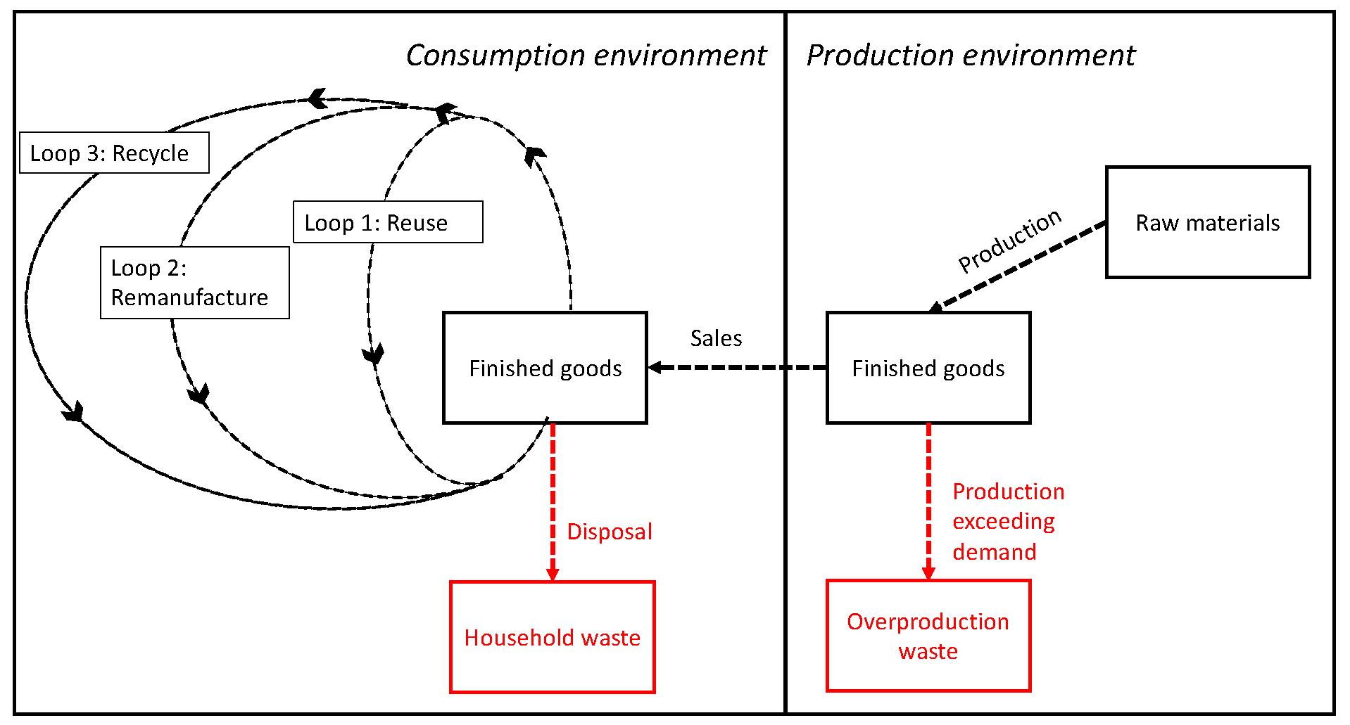
Our research is connected to two streams of the operations management literature: (1) circular operations management and (2) operational flexibility. One of the fundamental problems in the circular operations management literature is how to transform the linear “take-make-dispose” operational model to a circular structure, so that products can stay in the market after their lifetime to minimize waste on the consumption side [
13,
14]. The phenomenon of circular operations management is also known as closed-loop supply chain management (CLSC). There are three different layers of CLSC, which aim to minimize product waste on the consumption side. We depict these layers in
Figure 1.
The first layer of the CLSC is
reusing, which focuses on strategies to extend the consumption length of products [
14,
15,
16]. If a product is damaged or loses its functionality, it must be repaired to increase the length of the consumption period. When a customer loses interest in using a product, it must be sold in the secondary market or shared with other people. Therefore, the ease of repairing, resharing, and selling in secondary markets are key elements of the first layer [
14,
16]. One of the successful applications of reuse is the online marketplace of Patagonia, an outdoor apparel firm, where customers can exchange their clothes when they lose interest in them [
17]. Another example is the product ownership program of Xerox whereby the printing company retains ownership of the printers and leases them to customers [
14]. When a customer terminates its contract, Xerox leases the product to a new customer, so the company’s products are shared over their lifetime.
The second layer of the CLSC is
remanufacturing, whereby a set of refurbished and new components are used to manufacture products [
18,
19,
20]. There are two main challenges regarding the implementation of remanufacturing. The first is uncertainty about the flow of used components, which will later be refurbished for use in the manufacturing process. The second challenge is the cannibalization of the original items because introducing the remanufactured products to the market would result in lower sales of the original ones, leading to lower profits. Ref. [
19] address the first challenge by developing a queuing-theory model that dynamically estimates the flow of used products and then applying an aggregate base-stock policy to optimize the inventory policy. To address the second challenge, Ref. [
20] develop a diffusion model and categorize products depending on their market diffusion and purchase frequency. The authors outline a decision typology that shows the product categories with the maximum potential for remanufacturing.
The last layer of the CLSC is
recycling, whereby products at the end of their life go through a series of operations to manufacture new items. Well-known examples of recycling are paper and plastic recycling, which are observed in the recycling centers of municipalities of big cities. Yet, the most important challenge of recycling remains the collection of products from households. Ref. [
14] give the example of Norway, where the recycling rate for plastic bottles is impressively high—97%. Norwegians achieve this by providing government funds to support retail stores in collecting plastics via reverse vending machines (the same system can be observed in other western European countries such as the Netherlands). Another approach to increasing the recycling rate is to mandate manufacturers to develop collection and recycling mechanisms for their products, which is popularly known as extended producers responsibility (EPR) [
21]. EPR has been popularized in the electronics industry, with an example being the Minnesota Electronics Recycling Act [
22]. According to this act, the state of Minnesota imposes strict collection and recycling targets on producers as a percentage of their total sales volume [
22].
Studies in the extant literature successfully address the most important problems related to improving sustainability on the consumer side. Once a product reaches the market, keeping it in the loop of the CLSC has certain environmental benefits. However, the extant literature does not quantify the environmental impact of overproduction nor develop remedies for that problem. We contribute to the literature by filling this gap.
Our research is also related to a second stream of literature that prices the value of operational flexibility. Companies establish operational flexibility in different ways, such as lead-time reduction [
2,
8], quantity-flexibility contracts [
10], and multiple sourcing [
9,
23]. These operational-flexibility strategies make it possible for buyers to determine order quantities after the partial or full resolution of demand uncertainty, helping them to better match supply with uncertain demand. One of the challenges in the extant literature is related to demand modeling because the demand model should involve the time element in order to quantify the benefits of delaying the ordering decision. In practice, manufacturers often employ demand planning teams that collect credible information from customers and update demand forecasts over time. Thus, demand forecasts are improved over time as a result of such efforts. For this reason, the modeling approaches used in the operational-flexibility literature incorporate the evolutionary dynamics of demand forecasts in order to price the value of operational flexibility. Ref. [
8] use a multiplicative demand process to price the value of lead-time reduction. Ref. [
2] later extend the multiplicative demand model by incorporating sudden changes in the demand forecasts and show that the value of lead-time reduction increases with positive jumps in the demand forecasts. Ref. [
10] use a multiplicative demand model to price the value of quantity flexibility and show that the value is jointly affected by the order-adjustment flexibility and the time when the order adjustments are made. Ref. [
23] develop a tailored capacity model, which is analogous to the multiple-sourcing model that we consider in this research. In their model, a buyer utilizes a speculative capacity under demand uncertainty, but also reserves a reactive capacity that can be utilized once the demand is known. Ref. [
9] extends [
23] by using the extreme-value theory, so the tailored capacity model can be applied to a wider selection of product categories.
Our contribution to the operational-flexibility literature is that we quantify the environmental benefits of operational flexibility that appear in the form of reduced product waste during the sourcing process. The studies in the extant literature are based on a profit-oriented view of the firm such that a reduction in the supply–demand mismatch costs determines the value of operational flexibility. We hopefully expect that companies will be less concerned about increasing their profits in the future, focusing rather on understanding the environmental impact of their operations. Our research aims to fill this gap in the literature by showing how operational flexibility can help minimize product waste during the sourcing process.
3. Model Preliminaries
To quantify the impact of operational flexibility on excess inventory, we model the evolutionary dynamics of demand forecasts. There are two types of demand models that can be used for such a purpose: (1) the additive demand model and (2) the multiplicative demand model [
12,
24]. The
difference between the successive demand forecasts follows a normal distribution in the additive demand model, whereas the
ratio of the successive demand forecasts follows a normal distribution in the multiplicative demand model. It has been well established in the literature that the additive demand model fits the empirical data well when the forecast horizon is short and the demand uncertainty is low. However, the multiplicative demand model fits the empirical data well when the forecast horizon is long and the demand uncertainty is high [
24]. In this paper, we consider the multiplicative demand model because the lead times are expected to be long when companies source from offshore suppliers. Additionally, we focus on products with high demand uncertainty because the magnitude of excess inventory is more pronounced for products with high demand uncertainty than for those with low demand uncertainty.
We use
to denote the demand forecast at time
, such that
. The forecast-updating process starts at time
and ends at
. We fix
to the time when the actual demand is realized, so the final demand is fully known at
. Therefore, the length of the forecast horizon is
. The demand forecasts are updated at each time epoch
for
. According to the multiplicative demand model, the demand forecast
is formulated as follows:
The
term denotes the drift rate, and the
terms are the forecast adjustments that follow a normal distribution:
where
is the volatility parameter.
The drift rate can take non-zero values depending on the forecast-updating process. Ref. [
12] gives an example of a forecast-updating process such that demand planners use only the advance demand information to update the demand forecasts, which is modeled by a multiplicative demand model with a positive drift rate. When the forecasts are updated based on an unbiased judgmental demand process, the drift rate should be set equal to zero [
12]. The multiplicative demand model, given by Equation (
1), yields a lognormal distribution for the end demand, which is conditional on the demand forecast at
:
The location parameter of the lognormal distribution is , and the scale parameter is .
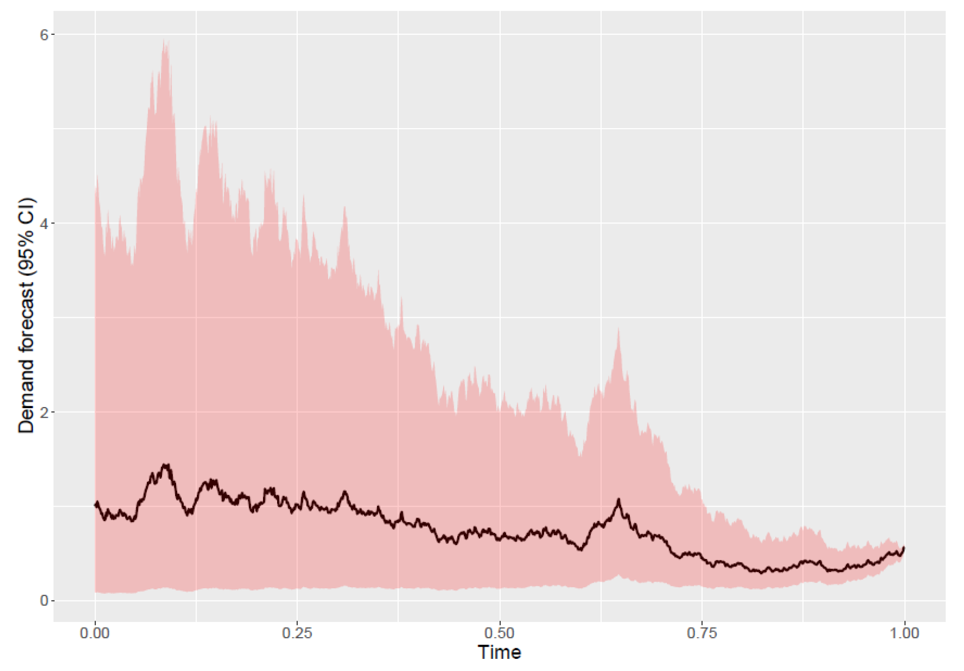
In
Figure 2, we present an example of the multiplicative demand model with a drift rate of zero and a volatility parameter of one. We normalize the initial demand forecast to one and scale the length of the forecast horizon to one. Thus,
,
, and
. We simulate a random path of the evolution of demand forecasts and calculate the 95% confidence interval over the forecast horizon. The black curve represents the demand forecasts, and the pink area shows the 95% confidence interval. For example, the demand forecast at
is equal to one, and the actual demand is expected to be between zero and four at
given by the limits of the pink area. As shown in the figure, the distance between the limits of the confidence interval decreases over time. This observation indicates that the accuracy of the demand forecasts improves over time as the time for the realization of the final demand approaches, which is consistent with practice. Therefore, the multiplicative model is very effective in capturing the dynamics of demand-updating mechanisms in practice [
12,
24].
We now apply the multiplicative demand model given by Equation (
3) to develop the expected profit, optimal order quantity, and expected excess inventory derivations. We consider the classical newsvendor model such that a buyer sells the products in a market with uncertain demand. We use
p to denote the selling price of a product per unit. The buyer incurs a purchasing cost of
c per unit. Unsold inventory is salvaged at a salvage value of
s per unit. The salvage value can be negative in some industries where companies pay to throw away the excess inventory. In the pharmaceutical industry, for example, unsold drugs must be destroyed after their shelf life because of strict regulations, making the salvage value negative for pharmaceutical companies. The critical-fractile solution was developed to determine the optimal order quantity in the classic paper of Arrow et al. [
25]:
where
is known as the critical fractile or the critical ratio. When the demand follows the lognormal distribution given by Equation (
3), the optimal order quantity is found by:
where
is the inverse of the standard normal distribution function
.
To find the expected profit, we first need to derive the standardized order quantity. When the buyer orders
Q units, the standardized order quantity becomes:
Then, the expected profit for an order quantity of
Q units is given by Bicer and Hagspiel [
10]:
The first term on the right-hand side of Equation (
7) gives the total profit when all the units ordered are sold in the market at the selling price. However, the demand is uncertain, and it can be less than
Q units. The second term on the right-hand side of the expression can be considered as the cost of an insurance policy that fully hedges the excess inventory risk. The term in brackets is the expected excess inventory:
The last expression indicates that the excess inventory (hence the waste) can be reduced using two different approaches. First, postponing the ordering decision leads to a reduction in the time window , which in turn helps decrease the expected excess inventory. Second, reducing the order quantity results in a decrease in the expected excess inventory.
These results provide useful insights regarding the use of operational flexibility to improve sustainability by reducing waste in the sourcing process. The lead-time reduction and quantity-flexibility practices make it possible for the buyer to postpone their ordering decision. Therefore, these two operational-flexibility strategies help decrease excess inventory. Utilizing multiple sources (one offshore supplier and one domestic supplier), the buyer can reduce the quantity ordered from an offshore supplier. Thus, multiple sourcing also helps reduce the excess inventory.
4. Analysis of the Impact of Operational Flexibility on Excess Inventory
We now look at the impact of the three operational-flexibility strategies (i.e., lead-time reduction, quantity flexibility, and multiple sourcing) on the excess inventory in order to quantify the environmental benefits of operational flexibility. The analytical derivations of the optimal policies for these strategies are given in detail in de Treville et al. [
8] for lead-time reduction, Bicer and Hagspiel [
10] for quantity-flexibility contracts, and Biçer [
9] for multiple sourcing. The following subsections first discuss the analytical derivations of the optimal policies for these strategies and then quantify the impact of operational flexibility on excess inventory.
4.1. Lead-Time Reduction
Suppose that a buyer purchases products from an offshore supplier and sells them in a market with uncertain demand. The buyer places the purchase order at time , and the products are delivered at time such that . The buyer sells the products in the market at time . This setting applies to fashion apparel brands that use contract manufacturers to make their clothes and sell them to retail stores at the beginning of each selling season. The length of is the decision lead time, which is the time elapsed between when the ordering decision is made and when the actual demand is observed. The demand is highly uncertain at time , which in turn exposes the buyer to excess inventory risk.
We assume that the selling price is
per unit, and the salvage value is
per unit. We use
to denote the cost of ordering from the offshore supplier per unit. Then, the optimal order quantity can be found by Equation (
5). When the buyer places the optimal order quantity, its expected profit and expected excess inventory can be found by Equations (
7) and (
8) conditional on the optimal order quantity.
We now consider the case that the buyer aims to reduce the lead time by switching to a local responsive supplier. This makes it possible for the buyer to place the order at time such that . However, the buyer incurs a higher purchasing cost when buying products from the local supplier. We use to denote the cost per unit of ordering from the local supplier such that . Therefore, the buyer is exposed to a trade-off between postponing the ordering decision and incurring a higher ordering cost. This trade-off has a significant impact on the buyer’s profits and the excess inventory.
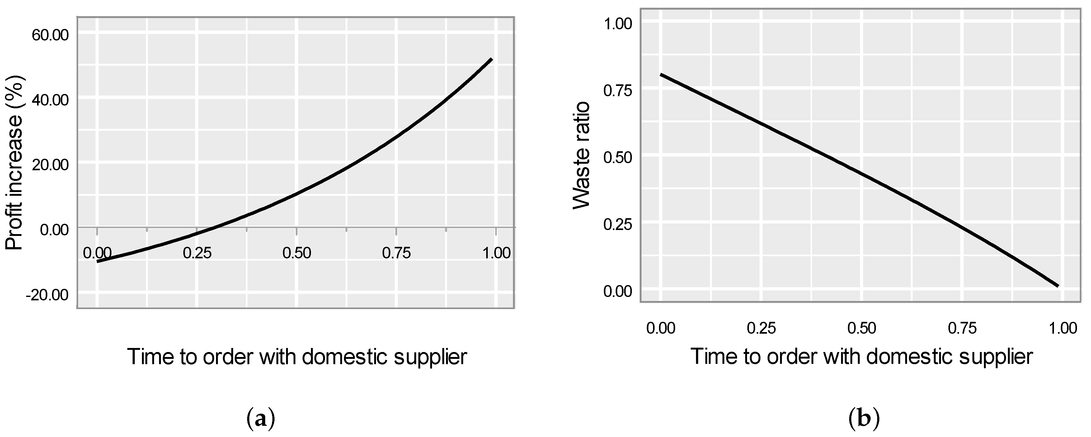
In
Figure 3, we present an example of a buyer who would like to decide whether to purchase products from an offshore or a domestic supplier. The selling price of the product is USD 300 per unit; the cost of purchasing from the offshore supplier is USD 40 per unit; the cost of purchasing from the domestic supplier is USD 50 per unit. Unsold inventory is thrown away, so the salvage value is set equal to zero. We normalize the initial demand forecast to one (
) and change the demand parameters accordingly. The drift rate of the multiplicative demand model is set equal to zero, and the volatility is equal to one. We also normalize the long lead time (i.e., when an order is placed with the offshore supplier) to one such that
by setting
and
.
We present the percentage change in profit in
Figure 3a when the buyer switches from the offshore supplier to the domestic supplier. The x-axis represents the time of ordering with the domestic supplier (i.e.,
), and the y-axis represents the percentage increase in profits. When the domestic supplier is not responsive enough, the benefits of local sourcing disappear, resulting in a loss of profit. As shown in the figure, the profit increase is negative when
. In this case, it is not advantageous for the buyer to order from the domestic supplier, so a buyer aiming to maximize profit would continue to source from the offshore supplier. If the domestic supplier is responsive enough to let the buyer postpone the ordering decision to later than
—that is,
—the buyer would increase their profit by switching from the offshore supplier to the domestic supplier. If the lead time is reduced by half (i.e.,
),
Figure 3a shows that ordering from the domestic supplier leads to a profit increase of around
. If the lead time is reduced by 90% so that
, the buyer can increase their profit by around
.
In addition to these economic benefits, the lead-time reduction helps the buyer reduce waste, thus having a positive environmental impact on the sourcing process.
Figure 3b shows the waste ratio, which is the ratio of excess inventory when the buyer orders from the domestic supplier to the excess inventory when they order from the offshore supplier. The x-axis represents the
value, and the y-axis represents the waste ratio. When
, the lead time for ordering from the offshore supplier is the same as the lead time for ordering from the domestic supplier. Even if the lead times are the same for both sourcing alternatives, the waste ratio is lower than one for
, meaning that local sourcing helps reduce waste even in the absence of a lead-time reduction. The waste ratio of
for
is a result of the difference in ordering costs between the domestic and offshore suppliers. The cost of ordering from the domestic supplier is more than ordering from the offshore supplier (
). This leads to lower ordering levels when the domestic supplier is used rather than the offshore supplier. Therefore, the 20% reduction in waste for
can only be attributed to the lower ordering levels, which is independent of the benefits of a lead-time reduction. However, this improvement is not attainable because
Figure 3a shows that the buyer prefers the offshore supplier over the domestic one when
.
When the
value increases,
Figure 3b shows that the waste ratio decreases. Therefore, the buyer can reduce waste during the sourcing process by cutting the lead time with the domestic supplier. When sourcing from the domestic supplier makes it possible to reduce the lead time substantially, the buyer reaches alignment between the economic and environmental incentives of local sourcing. On the one hand, the buyer can increase their profit due to better matching between supply and demand. On the other hand, they can also reduce the waste at source by minimizing the excess inventory. Apart from these direct benefits, promoting local production may also help improve the extent of remanufacturing and recycling because it increases product know-how in local markets.
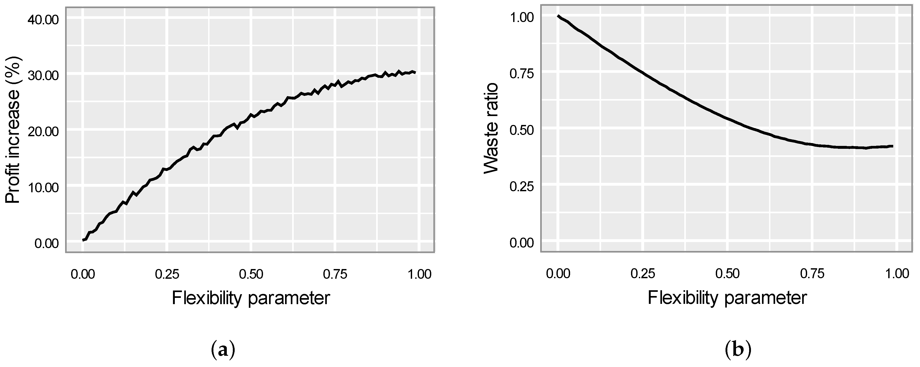
4.2. Quantity-Flexibility Contracts
When the buyer does not have the possibility of implementing local sourcing, a quantity-flexibility contract can be used to increase profits and reduce excess inventory. Under a quantity-flexibility agreement, the buyer determines the initial order quantity at time
and the flexibility percentage. We use
to denote the initial order quantity and following the terminology in [
10] we use
to denote the flexibility percentage. Then, the buyer determines the final order quantity
at time
within some limits:
If the demand forecasts are updated upward from
to
, the buyer would increase the order quantity up to
units. Otherwise, the buyer would decrease the order quantity down to
units. Thus, the final order quantity depends on the demand forecast at time
, the initial order quantity, and the flexibility percentage. It is given by [
10]:
where:
The
and
terms can be interpreted as the lower and upper critical values for the demand forecast at time
. If the demand forecast
turns out to be higher than
, the buyer should order the maximum allowable quantity based on the quantity-flexibility contract, which is equal to
units. If the demand forecast
turns out to be lower than
, the buyer should reduce the order quantity to the minimum allowable level, which is equal to
units. If the demand forecast
is between these limits, the buyer should set the order quantity to the profit-maximizing level. Based on the final order quantity, the expected profit and the expected excess inventory can be calculated by Equations (
7) and (
8), respectively.
In
Figure 4, we present an example of a buyer who orders products from an offshore supplier and has the flexibility to update the initial order quantity based on a quantity-flexibility contract. The cost parameters are the same as above: The selling price is USD 300 per unit, the cost of purchasing from the offshore supplier is USD 40 per unit, and there is no salvage value for unsold inventory. Likewise, the demand parameters are the same as above. The demand forecast at
is normalized to one. The drift rate and the volatility are equal to zero and one, respectively. The initial order quantity is determined at the very beginning such that
. The final order quantity is determined at
within the quantity-flexibility limits.
Figure 4a shows the impact of flexibility on the percentage profit increase. The x-axis represents the flexibility percentage
, and the y-axis represents the percentage increase in profits as a result of the order-adjustment flexibility. To calculate the values of the profit increase, we generate 100,000 random demand paths for each
value. We compare the demand realization at
along each sample path with
and
limits to determine the final order quantity. Then, the expected profit is calculated using Equation (
7).
Figure 4a demonstrates that the percentage change in profit increases with a decreasing rate as the flexibility increases. When
, the buyer can achieve around 20% profit increase compared with the no-flexibility case.
Figure 4b depicts the waste ratio as a function of the flexibility parameter. We calculate the waste ratio as the ratio of the expected excess inventory when the buyer has the flexibility to update the initial order quantity to the expected excess inventory when the buyer has no flexibility. Therefore, the waste ratio is close to one when the flexibility percentage is near zero. As the flexibility percentage increases, the waste ratio decreases with a decreasing rate. The curve becomes flatter for high
values such that the waste ratio cannot be reduced below 40%. These results indicate that quantity flexibility has positive economic and environmental impacts on the sourcing process of the buyer. However, its environmental impact is more limited than what can be achieved with lead-time reduction.
4.3. Multiple Sourcing
In the lead-time reduction and quantity-flexibility practices, the buyer can source products from only one supplier. In the former case, the buyer can source products from either an offshore supplier or a domestic supplier but not from both at the same time. In the latter case, the buyer can only order from an offshore supplier that provides the flexibility to adjust the initial order quantity in a later time epoch. We now consider an alternative strategy, whereby the buyer can source products from two different suppliers at the same time: One is the offshore supplier and the other the domestic.
The multiple sourcing strategy is very effective in mitigating the risk of supply–demand mismatches [
9]. By utilizing an offshore supplier, the buyer benefits from the cost advantages of offshore production. If the buyer orders lower quantities from the offshore supplier, the excess inventory risk can also be minimized. If the demand turns out to be unexpectedly high, the buyer then utilizes the domestic supplier to meet the surplus demand. Therefore, a multiple-sourcing strategy allows the buyer to benefit from the cost advantages of the offshore supplier and the responsiveness of the domestic supplier at the same time. However, one of the implementation challenges of this strategy is that the domestic supplier may not always be utilized at a high level. If the demand turns out to be low, the quantity ordered from the domestic supplier would not be high enough to fully utilize its available capacity. Therefore, domestic suppliers are exposed to the risk of capacity underutilization when a multiple-sourcing strategy is employed. To compensate for this risk, domestic suppliers often charge their buyers a capacity reservation fee.
To capture these dynamics, we consider a multiple-sourcing setting with one buyer, one offshore supplier, and one domestic supplier. The buyer determines the order quantity of
units from the offshore supplier and reserves a capacity of
K units with the domestic supplier at time
. We use
and
to denote the cost of ordering from the offshore supplier and the capacity reservation cost at the domestic supplier per unit, respectively. At time
, the buyer observes the final demand and determines the final order quantity of
units from the domestic supplier such that
. The domestic supplier is additionally paid
per each unit ordered. The formulation of
is given by Biçer [
9]:
where
is the final demand for the product, which is observed at time
. Following up from Biçer [
9], we first define two ratios to derive the optimal values of
and
K. They are:
Then, the optimal values are given by Biçer [
9]:
Then, the profit in the multiple-sourcing setting is formulated as follows:
Using this formula and simulating the demand paths, the expected inventory for the optimal
and
K levels can be found. The expected excess inventory can also be calculated by plugging
into Equation (
8).
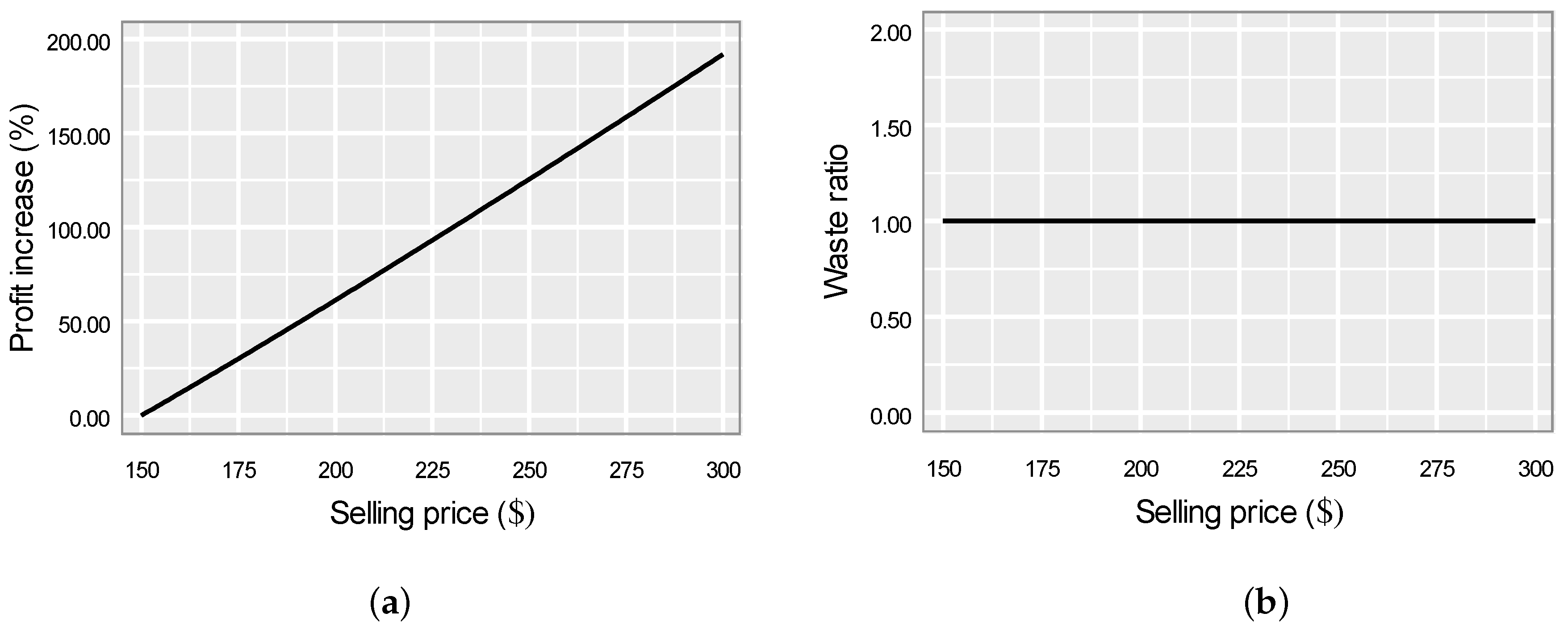
We now present an example to demonstrate the impact of multiple sourcing on the buyer’s profits and excess inventory. We assume the same demand parameters as the examples given above. The cost of purchasing from the offshore supplier is USD 40 per unit, and the cost of purchasing from the domestic supplier is USD 50 per unit. The domestic supplier also charges USD 15 for each unit of capacity reserved. Unlike the lead-time reduction and quantity-flexibility examples, we cannot vary the key decision parameter that determines the magnitude of operational flexibility in the multiple-sourcing setting. In the multiple-sourcing setting, operational flexibility is directly influenced by the reactive capacity K. However, the reactive capacity is not a control variable. It is a decision variable that has to be optimized depending on the cost and demand parameters. For that reason, we vary the selling price between USD 150 and USD 300 in our analysis because Equation (17) indicates that the optimal capacity level increases with the selling price. In other words, we can observe the impact of responsiveness on profits and the waste ratio by varying the selling price because the selling price is directly correlated with the capacity level.
Figure 5a shows the impact of the selling price on the percentage profit increase such that the profit increases with the selling price. Doubling the selling price from USD 150 to USD 300 increases the profit by almost 190%.
Figure 5b demonstrates that the waste ratio does not change depending on the selling price. This is because the optimal order quantity from the offshore supplier does not depend on the selling price but only on the cost parameters. For this reason, there is no environmental benefit to improving operational flexibility with the multiple-sourcing strategy. Both the profit increase and waste ratios in
Figure 5a,b are calculated with respect to the resulting profit and waste when the selling price is set at USD 150.
We summarize the results of the three operational-flexibility strategies in
Table 1 below. For each strategy, the profit increase and waste ratio reported are calculated by setting the parameter of the strategy in the table to the maximum value in comparison to setting the parameter to the minimum value within the given range. The results show that lead-time reduction has the highest potential in reducing waste while improving the profits of companies. In
Section 5, we further elaborate on and discuss the results of the three strategies.
5. Discussion
So far, we have shown the effect on the change in profit and the waste ratio of three supply chain flexibility strategies: (1) lead-time reduction, (2) quantity-flexibility contracts, and (3) multiple sourcing. The numerical analysis of lead-time reduction shows that when a firm reduces its lead-time by utilizing an onshore supplier instead of an offshore supplier, the firm can achieve both profit increase and waste reduction due to the decrease in demand uncertainty at the order time. When is greater than 0.29, the firm starts experiencing a positive change in profit, which exceeds 50% as increases to 1. As for the waste, even if , the firm still experiences waste reduction of 20% due to the increased cost, which lowers the newsvendor order quantity. The waste ratio decreases to zero as increases to one, since the actual demand is known at this point and the firm does not operate under demand uncertainty anymore.
If firms cannot order from an onshore supplier, they can still benefit from the flexibility of an offshore supplier with a quantity flexibility contract where, up to time , the firm can still adjust its order quantities by a factor of . For a fixed , our analysis shows that firms can achieve a 30% increase in profit, and waste reduction can reach more than 50% as the flexibility parameter increases to 1.
For multiple sourcing, the numerical analysis is performed based on the selling price of the product. It shows that doubling the selling price from USD 150 to USD 300 results in a profit increase of almost 190%. The waste, however, does not change with different pricing as it is calculated based on the offshore order quantity, which is independent of price.
The selection of a given flexibility strategy is also dependent on the risk associated with it. On the one hand, although single sourcing with lead-time reduction has the highest effect in reducing waste while still increasing a firm’s profits, it can amplify the exposure to risk in the presence of uncertainty. On the other hand, multiple sourcing can present higher costs, and this is not accounted for as a result of having to manage several suppliers [
26]. It is therefore critical for firms to assess all the benefits and risks arising from choosing a specific strategy in pursuit of improved sustainability and profits.
6. Conclusions
Improving sustainability in every aspect of our lives is vital to safeguard a durable future for the next generation. Manufacturers ought to pay special attention to sustainability because what they produce, how they produce, and where they produce has a substantial impact on the carbon footprint. The extant literature on sustainable operations management mainly focuses on the consumption side of product life cycles, with an intention to extend the product lifetime and reduce household waste. However, significant inefficiencies exist on the production side of product life cycles, whereby manufacturers overutilize the Earth’s limited resources and generate carbon emissions when producing products in excessive amounts. A significant number of these products may never reach consumers. Prominent examples reported in the media include Amazon destroying thousands of unsold TVs and laptops in one of its warehouses [
27].
In this research, we aim to fill the gap in the literature by demonstrating how operational flexibility can help organizations achieve sustainability at source. We focus on three different operational-flexibility strategies: (1) lead-time reduction, (2) quantity-flexibility contracts, and (3) multiple sourcing. Our results indicate that lead-time reduction has the highest potential to reduce waste while improving the profits of companies. Therefore, operational-flexibility strategies that promote local production are key to reducing waste and improving sustainability.
In particular, in our numerical analysis, where ordering time varies between 0 (start of planning horizon) and 1 (beginning of sales season), we show that lead-time reduction can result in a profit increase when orders are placed with onshore suppliers at a time greater than 0.29, compared with being placed with an offshore supplier at time . The profit increase can go up to around 40% when orders are placed at , even if ordering costs are higher. Waste in terms of excess unsold inventory also decreases, even when when the onshore supplier is used, and results in a 20% waste reduction compared with ordering from an offshore supplier as a result of the higher ordering costs, which result in lower order quantities. The waste decreases as increases and finally approaches zero when orders can be placed during the selling season, when .
The results of our research offer some useful insights regarding the development of effective environmental policies. Because lead-time reduction is the most effective strategy, environmental policies should target cutting lead times, not only for inbound but also for outbound logistics. Increasing the import and export tariffs and imposing trade barriers would force countries to promote local production, which in turn leads to shorter lead times and lower waste. Although such policies conflict with the free trade and economic development ideas, we envision that environmental concerns would be highly dominant in the near future and governments would incrementally pass some regulations to reduce the volume of imports and exports. One of the side benefits of local production would be to establish a close connection between local manufacturers and local authorities such that recycling and remanufacturing can be easily implemented near the market bases. Therefore, local production may also help increase the product life cycle along the stages of the closed loop supply chains (
Figure 1).
One of the limitations of our research is that we mainly focus on the dynamics on the production side of the product life cycle without connecting it with the consumption side. We mainly consider a newsvendor setting such that the buyer sells the products in the market at a certain price. The classical utility theory [
28] suggests that the life cycle of a product is positively associated with the price paid for it. We believe that there is a need for empirical research that investigates the relationship between price and the length of a product’s lifetime in the retail industry for different categories. We envision that this would be an interesting avenue for further research.
Another direction for future research is how digital transformation could contribute to lead-time reduction. Recent research focuses on lean manufacturing in the Industry 4.0 era [
29]. Studies on lean manufacturing show that lead-time reduction is an important factor that enhances reliability and flexibility while decreasing inventory carrying costs and that integrating lean management and collaboration in the supply chain has important social, environmental, and economic benefits [
30]. Therefore, we foresee that studies of the effect of Industry 4.0 on decreasing waste and increasing profit through lead-time reduction are a potential field for future work.


