Article

Analysis of Bus Fare Structure to Observe Modal Shift, Operator Profit, and Land-Use Choices through Combined Unified Transport Model

1
Division of Environmental Design, Graduate School of Natural Science and Technology, Kanazawa University, Kakuma-machi, Kanazawa 920-1192, Japan
2
Faculty of Transdisciplinary Sciences, Kanazawa University, Kakuma-machi, Kanazawa 920-1192, Japan
3
Faculty of Geosciences and Civil Engineering, Institute of Science and Engineering, Kanazawa University, Kakuma-machi, Kanazawa 920-1192, Japan
*
Author to whom correspondence should be addressed.
Sustainability 2022, 14(1), 139; https://doi.org/10.3390/su14010139
Submission received: 31 October 2021 / Revised: 2 December 2021 / Accepted: 18 December 2021 / Published: 23 December 2021
(This article belongs to the Special Issue Sustainable Urban Design: Urban Externalities and Land Use Planning)

Abstract

:
In order to design sustainable urban transport systems, the inclusion of the behaviors of different stakeholders is imperative. In this study, we formulated the interactions of behaviors between transport operator, landowner, workplace, residence, route and mode choices, and location of firms and businesses through a combined unified model of land-use and transport system. The commuters have two mode choices for traveling: private car and public bus. They are inclined to choose a transit mode with minimum traveling costs. We combined two models, maximization of operator profit constrained by bus frequency, while maintaining the formulation of other stakeholders through an assignment sub-model. The resulting formulation is bi-level, which is optimally solved for a small-sized instance containing two zones. The findings suggest that if the bus fare is reduced, the demand of public bus is increased. However, the operators’ profit is optimized within a certain range of fares and is lowered when the fare is too low or too high. It is determined that maximum bus frequency does not guarantee maximum profit to the service operator. The impacts of traveling costs on residence choice behavior suggest that if link fares are more, many of people opt not to travel between different zones. The analysis results presented in this paper are calculated for two types of link fares: a fixed fare (30 currency), and a range of link fare (5 to 100 currency). Different variants of the same formulation can be applied for real settings to better comprehend the nature of the model and its applications.

1. Introduction

In recent decades, the growing demand for transportation has threated the sustainability of the cities because of excessive dependence on personalized automobiles. The increase in the private automobiles cannot efficiently cover the increased demand for transportation because of the associated concerns of traffic congestion, environmental pollution, and other health and safety issues [1]. Many measures can be adopted to restrict the growing demand for cars in urban areas. Public transport is one of the most important measures to reduce the dependency on personalized automobiles. In comparison with the performance of private cars, public transit systems (public bus) can outperform them in an environmentally friendly, efficient, and more sustainable manner [2]. For example, the use of public transport can be encouraged by improving the level of service (LOS), reducing the travel costs of commuters, providing government subsidies, re-adjusting the bus fares, or providing ‘Park and Ride’ (P & R) facilities which are gaining considerable attention among public transport systems to alleviate traffic congestion—especially in city centers [3,4,5]. However, in most cases, the mode choices are made under the assumption based on the maximization of utility. While the transport system does not only include travelers, but public transport companies (service operators) and governments. However, in many cases, public transport operators/companies traditionally balance their revenues and expenses. These public transport operators try to maximize their revenues at the expense of increased fares, which eventually deteriorate the quality of the service and as a result, people prefer to use personalized vehicles for commuting [6]. In practice, the full advantage of these public transit systems is not taken because of the imbalanced trade-offs between the commuters and the public transport service operators. It is necessary to devise a strategy with a strong connection between different stakeholders and their conflict of interests should be taken into consideration very carefully. This can be accomplished by the effective use of the strategies which open new opportunities to further benefit users, as well as operators, while ensuring that each stakeholder does not exceed the desired costs of traveling and operating the service, respectively. The potential users are likely to find the use of public bus attractive if fares are low and level of service is high [7]. Alternatively, service operators will discontinue the service if operation costs exceed the revenue. Therefore, an optimal combination of fares and LOS (bus frequency) is needed to be determined for the optimization of the total benefits of the users and service operators.
The sustainability of urban transit systems also depends upon how well connected the connections between different stakeholders are in the system to better explain their behavior in decision making. It influences the dependence of different decision-makers and related equilibrium results. For example, in a public transport system, it is necessary to consider the interaction between users as well as service operator for finding a fare system which benefits both stakeholders [8]. A review of the literature reveals that whenever it comes to the design and improvement of the public transport systems in urban settings, it is complex and needs many factors to be considered [6,9]. For example, the efficiency of urban public transport depends upon the traveling costs and operating frequency (LOS). By adjusting the service frequency (LOS), the demand of the users can be accommodated and service revenues can be optimized, which depends upon the number of users using the public transport system [10]. The traveling costs can be saved significantly if the re-organization of bus fares and bus frequency is done to accommodate the actual demand [7,11]. However, the re-structuring of the bus fare and transit route frequencies is one of the main aspects in the design and sustainable operations of the transit network [2,9,11,12,13]. The optimization and design of urban transit fare structures has been studied by many researchers from the perspectives of transport economics [14] and network equilibrium [15]. Harris et al. [16] proposed a fare elasticity model for the prediction of ridership and revenue from fare changes. Cummings et al. [17] studied the change in the ridership in the city of Chicago before and after the implementation of a fare changes strategy in the transit system. Wang et al. [18] inferred that fare structure significantly affects the demand of the users in public transport systems, with low fares causing deficit and high fares affecting social welfare. Similarly, Jin et al. [19] confirmed that increasing the fare structure can suddenly reduce the demand, service frequency, and ridership of public transport systems if attractive competing transport modes are available to the users. Lam and Zhou [20] presented that optimal fare and service frequency significantly affect the demand and route choice behavior of the users in a transport system. Since fares are one of the important parameters which affect the operators’ profit and users’ travel choices; therefore, the implementation of fare differentiation is one of the important aspects for practical implementation.
However, most of the existing studies consider travel time and cost-related attributes as explanatory variable to determine the quality of the transit service for attracting users and maximizing the operators’ profit. Most of the research studies which investigated the travel pattern of the users tried to minimize the operators’ as well as users’ costs as a common objective function. The models which jointly optimized different objectives using combination of different variables are shown in Table 1.
As it is evident from the literature mentioned above, most of the researchers tried to model the relationships between service operators and commuters. However, in this study, the land-use choices based on link fare are also discussed. The method proposed in this research study recognizes the interactions between different stakeholders for the optimization of service operators’ profit with bus frequency as a decision variable. While the role of stakeholders is modeled in the sub-assignment nested logit model. This research study covers several objectives, such as (a) maximization of service operator profit, (b) minimization of users’ traveling costs, (c) interaction behavior between different stakeholders in the transport system, and (d) sensitivity of the model against important variable such as link (bus) fare. Additionally, the relationship between mode choice (private car and public bus) and land-use changes are also evaluated, which makes this study unique from the existing body of the literature. Therefore, it is necessary to choose a combination of bus fare to benefit the whole system to meet the needs of the relevant stakeholders and factors for its critical development as a sustainable transportation system. In this research paper, the profit of service operators and the travel costs of commuters are solved in bi-level optimization manner. This paper utilized bi-level optimization for the efficient design of urban bus transit system. In the upper level of optimization, the profit of the bus operator is maximized which is subject to the bus frequency. However, in the lower level of optimization, the users’ cost is minimized as a sub-assignment model. The other behaviors—such as workplace, residence, route and mode choice, and firms and landowners’ behavior—are also formulated.
The rest of the research paper is divided into following sections; after the introductory section and literature review, Section 2 presents the model formulation and the behavior of different stakeholders, Section 3 describes the simulation results of simple example problem. Finally, Section 4 summarizes the conclusions and future research directions are presented.

2. Model Assumptions and Behavioral Formulation

2.1. Modeling Assumptions and Hypothesis

For the sake of simplicity, a simple transit network is considered in this research study and some of the modeling assumptions which are adopted are presented as follows:
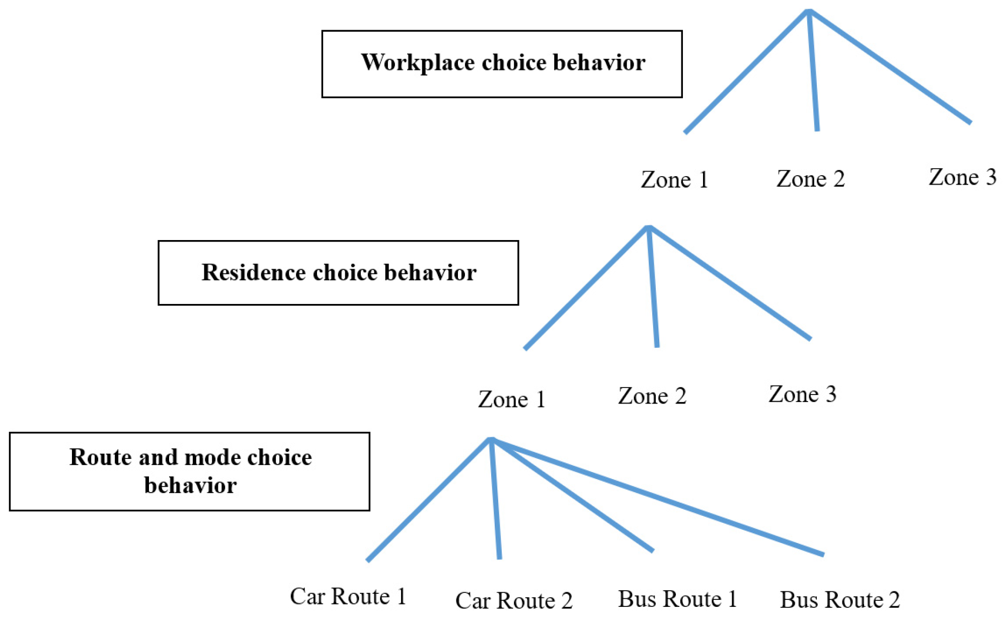
  • A1: Each user first chooses a workplace, then residence place and then route or mode choice is made. Before starting a journey, each user chooses a travel strategy (i.e., private car or public bus), depending upon minimum travel costs. Figure 1 shows the workers’ choice structure.
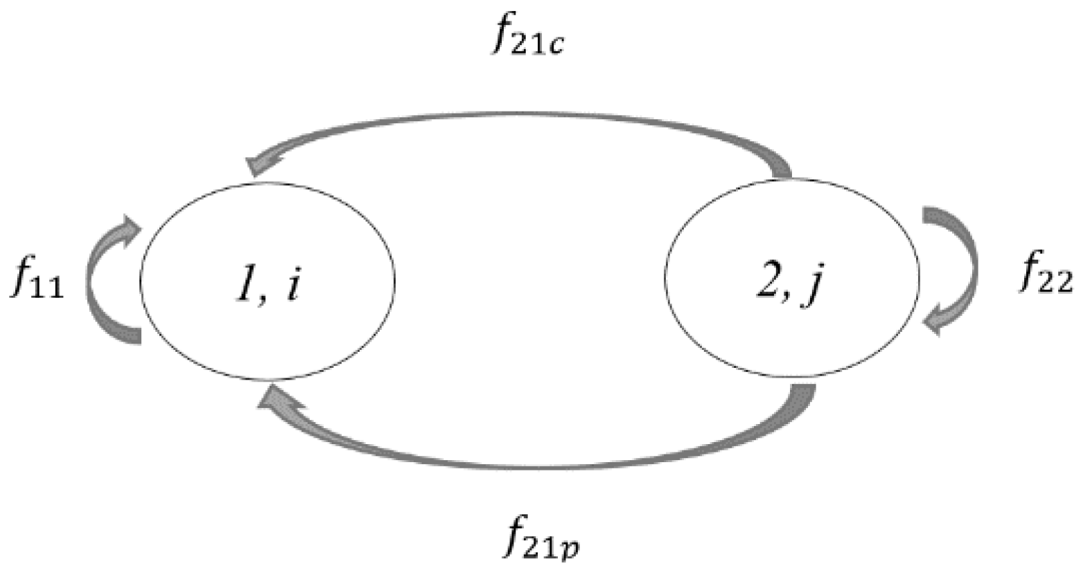
  • A2: Only commuting trips are considered in this modeling process in the peak time period for simplicity purposes. The overall traffic demand q i j is given between any Zones i and j.
  • A3: In this modeling process, firms, households, and landlords are considered homogenous. Each of the decision maker is considered homogenous for the sake of simplicity and their behavior is modeled as multinomial (or nested) logit structure. From each household, a single worker makes a commuting round trip daily.
  • A4: A firm chooses its location based on random profit, V i λ w i γ r i + ε i , where V i is the production of the firm in Zone i, λ is the number of workers in each firm, W i is wage in Zone i, γ is the area of land used by each firm, r i   is the rent for commercial lot in Zone i, and ε i is an error term.
  • A5: The profit of public bus operator is measured as a function of number of passengers, route length, fare rate (currency/km), operation cost, and number of vehicles.
  • A6: The transport service revenue is proportionate to passenger-km (bus passenger flow) traveled but operations costs depend upon vehicle-km traveled.
The proposed model has quite a good number of variables. However, in this research study, a simple transit network case is solved in order to understand the behavior of the model (Figure 2). Solving a simple case example is important to know the behavior of the model for a larger transport network. Because of the implications of a simple network can help in determining the transit policy for a larger and real-case network. It is pertinent to mention here that extending this model to a larger transport network is possible; however, because of the computational costs, it can be a challenging task. Additionally, the exact estimation of the input parameters is inevitable for concrete policy suggestions. The proposed model can be applied to evaluate the total benefit of the transport system which have different stakeholders by reducing users’ minimum travel costs and optimizing the benefit (revenue) of the public transport operator. This model can be applied to modify the service frequency on the public transport routes to optimize the transport system performance. Different variants of the same formulation can be applied for real settings to better comprehend the nature of the model and its applications.

2.2. Behavioral Formulation

2.2.1. Work Choice Behavior of Employees

The work choice location behavior of the employee depends upon the maximum wage and minimum expected cost of travel between different zones. It is important to consider that the minimum expected cost, σ i , is estimated based on the rent in Zone i and commuting costs between pair ij.
y i = N exp { θ 3 ( σ i w i ) } l Z exp { θ 3 ( σ l w l ) }       i Z
where, y i is the number of employees commuting in zone i, N is the total number of employees in all zones, σ i is expected minimum cost in Zone i (log-sum value of residence choice behavior), w i is the wage rate, θ 3 is the logit parameter, and Z is a set of Zones.

2.2.2. Residence Choice Behavior of Employees

The residence choice shows the number of workers who reside in Zone j but work in Zone i and it depends upon the rent and commuting cost between ij.
q i j = y i exp { θ 2 ( r j + σ i j ) } l Z exp { θ 2 ( r l + σ i l ) }       ( i , j ) Z × Z
σ i = 1 θ 2 ln l Z exp { θ 2 ( r l + σ i l ) }       i Z
where, q i j is the demand of the residents traveling between Zone i and j, r j is the rent in Zone j, σ i j is the expected commuting cost between Zone i and j (log-sum value of route and mode choice behavior), and θ 2 is the logit parameter.

2.2.3. Route and Mode Choice Behavior of Employees

The users always try to choose the mode (private car or public bus), which minimizes traveling costs. The route flow of path k can be formulated as
f i j k = q i j exp { θ 1 c i j k } k K i j exp { θ 1 c i j k }     k K i j     ( i , j ) Z × Z
σ i j = 1 θ 1 ln k K i j exp { θ 1 c i j k }
where, f i j k is the flow of commuting from zone j to zone i in route k .   c i j k is the measured travel cost of route k , K i j is the path set between Zone pair ( i , j ) and θ 1 is a logit parameter. If private car is chosen as a preferred mode, the route set is defined as, K i j , car and K i j , bus otherwise in the case of public bus. The costs of traveling by using private car and public bus are given as
c i j k = { a A i j , k t a ( x a ) + P k if   k K i j , car a A i j , k t a ( x a ) + X k + 30 v k if   k K i j , bus
where, t a ( x a ) is the travel time of link a and A i j , k is the link set of path k = c, p . This travel times are the function of link travel volume x a for considering the road congestion. P k is the driving and traveling costs for private car including the fuel cost, car parking cost (currency), and maintenance cost. X k is the bus fare, and v k is the frequency of bus service. K i j , car and K i j , bus are the path set of private car and public bus, respectively. The link travel time (BPR) functions t a ( x a ) can be formulated as follows:
Free flow time,
t a ( x a ) = t 0 , a { 1 + α a ( x a C a ) β a }
where, t 0 , a is free flow travel times, C a is the capacity of link a , and α a ,   β a are the parameters related to congestion effects.
x a = i Z j Z k K i j δ i j k , a f i j k
In Equation (8), δ i j k , a is a link-route incidence indicator, which is 1 if link a belongs to route k between OD pair ij, and 0 otherwise.

2.2.4. Firms’ Behavior

For modeling firms’ behavior, we consider that they select the land-use with highest profit, (higher productivity, lower rent, and lower wage rate). In reality, there exist different types of firms which are engaging in diverse businesses, but we consider them homogenous. In other words, we can say that as our prime objective is to observe the land-use so only firm’s activity is focused. The profit of the firm is measured by Equation (10). Therefore, the number of firms in Zone i can be calculated
m i = N λ exp { κ π i } i Z exp { κ π i }       i Z
π i = V i λ w i γ r i         i Z
where, m i is the number of firms in Zone i, π i is firms’ profit in Zone i, V i is the production volume in Zone i, λ is the number of employees in one firm, γ is the land required by one firm, r i represents the business rent of firm in Zone i, and κ is a logit parameter.

2.2.5. Landowners’ Behavior

It was formulated that the landowner uses land for the purpose of residence or business. It was supposed that the area used for residential purpose is one unit. The landowner can decide the rents and land use assignment for maximizing their random utility. Therefore, the area of each zone used for different purposes can be determined by the following equations
l i = D i e μ r i e μ r i + e μ r i       i Z
where, l i and l i are the areas of residential and businesses lots in Zone i,  D i is the total area of Zone i, r i   ( or   r i ) is the rent of the residential (or business) area, and μ is the logit parameter for this choice behavior.

2.2.6. Total Quantity Conditions

As assumed earlier, each zone contains homogeneous type of firms, indicating that each firm has same number of employees λ . Based on the assumption, the number of employees can be equilibrated with the urban area, meaning that total number of employees divided by the total number of firms is equal to the number of employees in each firm. This assumption equilibrated the supply and demand in each zone.
i I q i j = l j       j Z
γ m i = l i       i Z
λ m i = y i       i Z
D i = l i + l i       j Z
k K i j f i j k = q i j       ( i , j ) Z × Z
j Z q i j = y i       i Z
i Z y i = N
f , q , y , m , l , l 0
In Equation (20), f , q , y , m , l , l represent the vectors of flow, demand, number of employees, number of firms, residential area, and business area, respectively. It is indicated that the total number of employees working in Zone i are equal to the number of employees in one firm in Zone i times number of firms in Zone i. It is pertinent to mention that Zone i ( Z ) and Zone j ( I ) .

2.2.7. The Unified Equilibrium Model Formulation of Three Players

Assuming that the conditions for public transportation ( v k , X k ) are given; where v k represent the bus frequency (number of vehicles on route) and X k represents the bus fare. The unified equilibrium model (including transportation network, firm location, residential/workplace location decision, and land/labor market) can be formulated as the following optimization problem.
min f , q , y , m , l , l S ( f , q , y , m , l , l | v , X )
s.t. Equations (13)–(20)
S ( f , q , y , m , l , l | v , X ) = a A 0 x a t a ( u ) d u + 1 θ 3 i Z j Z k K i j f i j k ln f i j k q i j + 1 θ 2 i Z j Z q i j ln q i j y i + 1 θ 1   i I y i ln y i N i Z m i V i + 1 κ   i Z m i ln λ m i N + 1 μ   i I ( l i ln l i D i + l ' i ln l ' i D i   )
Note that we have not dealt with rent ( r i , r i ) and wage ( w i ) in this optimization model. These variables can be derived by solving the dual problem of this problem for satisfying the Equations (1)–(20). However, in this research study, the authors mainly focused on the workplace, residence, and commuting (route and mode choice) behaviors of the users. The behavior of the service operator is also formulated to check the sustainability of the public transport system. Therefore, the duality problem for the calculation of rent ( r i , r i ) and wage ( w i ) is not discussed in this research study.

2.2.8. Bus Operator Behavior
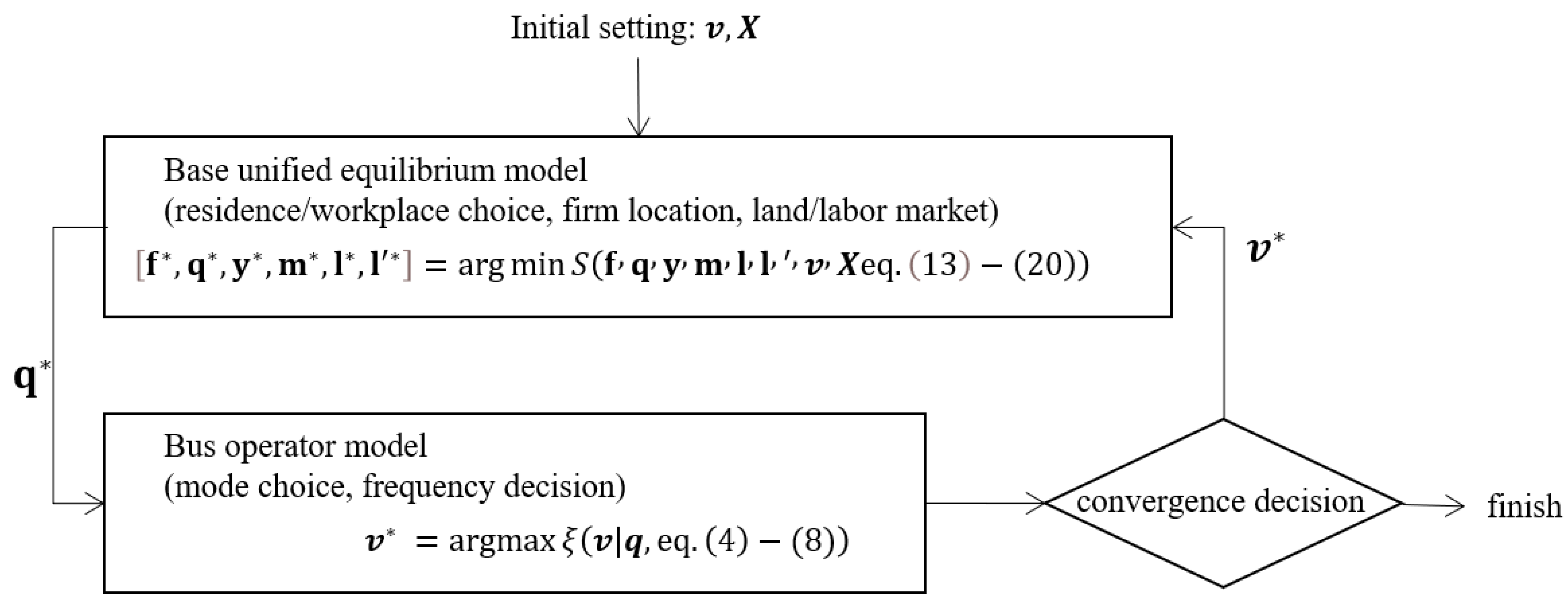
The bus frequency v k is controlled by the bus operator which want to maximize the profit. We assume that the bus operator cannot determine the fare. Therefore, bus operators will always try to maximize the revenue which is directly related with demand of bus. Here, the bus frequency affects the travel demands as the waiting time (30/ v k at Equation (6)).
The profit function of bus operator can be formulated as
ξ ( v k ) = i Z j Z k K i j , bus f i j k ( v k ) X k C k v k
where, C k is the bus operation cost per one frequency at route k . Then, the bus operator behavior (profit maximization) can be formulated as
max v ξ ( v k | q )
s.t. Equations (4)–(8)
v k f i j k C bus     if   k K i j , bus
Here, residence and place of work q , which do not change in the short run, are formulated as given. Equation (25) means the bus capacity constraints, C bus indicates the capacity of one bus service.

2.3. Algorithm

In this paper, we deal with a unified equilibrium that includes public transport operators by solving two types of optimization problems alternately. Hence, the equilibrium conditions for an arbitrary set of fares X k will be derived by the algorithm shown in Figure 3. It should be noted that this calculation does not guarantee the uniqueness of the solution and may depend on the initial values. This paper discusses one of the calculated equilibrium solutions. The solution algorithm of the combined model of unified equilibrium and bus operator is shown in Figure 3.

2.4. Sample Transit Network

The model has quite a good number of variables. However, in this study we tried to explain the model with the help of a simple example for the sake of improving the understanding. In this study, two transport modes (private car and public bus) are considered in the transit network between two Zones i and j, as traffic assignment model. It is considered that people choose to live in Zone j and they work in Zone i. Zone i is a Central Business District (CBD) and Zone j is a suburb. The travelers have two options for traveling—i.e., private car and public bus—they will always choose an option with minimum traveling costs. The traffic flow by private car is represented as f 21 c , while the traffic flow by public bus is represented as f 21 p (Figure 2). In addition to this, the cost of traveling by private car includes the travel time (traveling costs and maintenance cost), fuel cost, and the parking cost. The travel cost by public bus includes the travel cost, waiting time cost, and fare. The waiting time in the formulation of travel cost by public bus is done to increase the realism of the transit network. The simulation results are coded in MATLAB version 2018a and run-on personal computer Intel(R) Core™ i5-4590 CPU 3.30 GHz, 16 GB RAM, and Windows 10 Education with 64-bit Operating System. A simple example of the sample transit network to explain the model is shown in Figure 2.

2.5. Parameter Setting

This simple transit network is defined as shown in Figure 2 and other parameters required for the sake of simulation were set (Table 2). The length of the route between Zone 1 and 2 is same for both car and bus. Bus operation cost is added as 400 which is fixed and covers the overhead charges, maintenance cost, and the fuel cost of service operation. The waiting time of bus is set as 30/ v k (Equation (6)) and the fare is set between 5 to 100 currencies to check the simulation results between zones for the sake of understanding the behavior of the model. The total number of households and total number of firms in both Zones 1 and 2 are set as 20,000 and 1000, respectively. The residents are free to choose the mode for commuting between Zone 2 and 1. However, it is assumed that they will choose the mode which minimizes their traveling cost. In other words, the cheapest mode of transport is always preferred mode of choice between both zones. The car fuel cost is set as 10 currencies and it do not include any waiting time, while contrary to that waiting time cost has been included in the case of bus travel cost to increase the realization of the transportation network. In each mode, the travel cost basically has three components, the congestion cost (BPR function), the travel cost (fuel or fare cost or maintenance cost), and the waiting time cost. It is important to mention that the setting of the parameters is not exact estimation, therefore, concrete policy recommendations based on these results are not possible. It is assumed that all the firms have similar numbers of workers, and the firm sizes are also the same. In this study, we only intend to check the basic behavior of the model. In order to give concrete policy recommendations, accurate estimation of the parameters is required. In the upper level of this bi-level optimization, operator profit is maximized, which is the revenue minus the operation cost of the fleet. In the lower level of optimization, traffic sub-assignment model is formulated which include the behavior of all stakeholders. The parameters set for the modeling are shown in Table 2 as follows:

3. Results and Discussions

3.1. Simulations with Fixed Fare ( X k = 30)

As it has been mentioned earlier that the model has quite a good number of variables. Therefore, in order to improve the understanding of the model, a simple network example of including two zones has been solved. The simulations are carried out for (a) fixed fare of 30 (currency) and (b) variable fare for a range from 5 to 100 (currency), which is discussed in the next sub-section. Zone 1 is considered as the CBD while Zone 2 is mainly a suburban area. The total areas of Zone 1 and Zone 2 are 1000 m2 and 2000 m2, respectively. Both of these zones are connected via two links, private car and public bus. f21c and f21p represent the flow of private car and public bus between Zone 2 and Zone 1, respectively. The link flow times between zones are calculated, which are 53.314 and 20 by private car and public bus, respectively.
The optimization of the model yields the number of variable outputs as listed in Table 3. It is important to mention here that each firm has uniform number of workers ( λ ) and uniform area ( γ ). Solving the model yields that the total demand of travelers who commute from Zone 2 to Zone 1, is q21 = 332.766, where the number of people who opt to use private car and public bus for commuting are 149.352 and 183.414, respectively. It is apparent from Table 3 that as the travel cost for commuting between Zone 2 and Zone 1 is less in case of public bus; therefore, a greater number of people choose to travel by public bus. Table 3 also shows other variables which are calculated from the model such as residential and business areas, residential and business rent, and number of households and number of employees in Zone 1 and Zone 2. As Zone 1 is treated as a CBD, the business rent and wage in Zone 1 are higher as compared with Zone 2. Contrary to that, Zone 2 is treated as suburban; therefore, the residential rent and business rent in Zone 2 are less as compared with Zone 1. As business rent in Zone 1 is higher, which affects the profit of the firms (Equation (10)), therefore in order to maximize the profit, many of the firms opt to choose Zone 2. As the business rent and wage rate in Zone 2 is less, which attracts many of the firms to choose Zone 2. On the other hand, as the residential rent in Zone 2 is lower, approximately 56% of the households choose to live in Zone 2. It is pertinent to mention that wage and rent in both of the zones are calculated endogenously. It can be seen from Table 3 that both residential and business rent in Zone 1 is higher as compared to Zone 2, which leads to the fact that many of the households and firms choose Zone 2. The detailed results of the model output parameters are shown in the following Table 3. This confirms the fact that this unified model has the ability to model the transportation network and land use equilibrium problem.

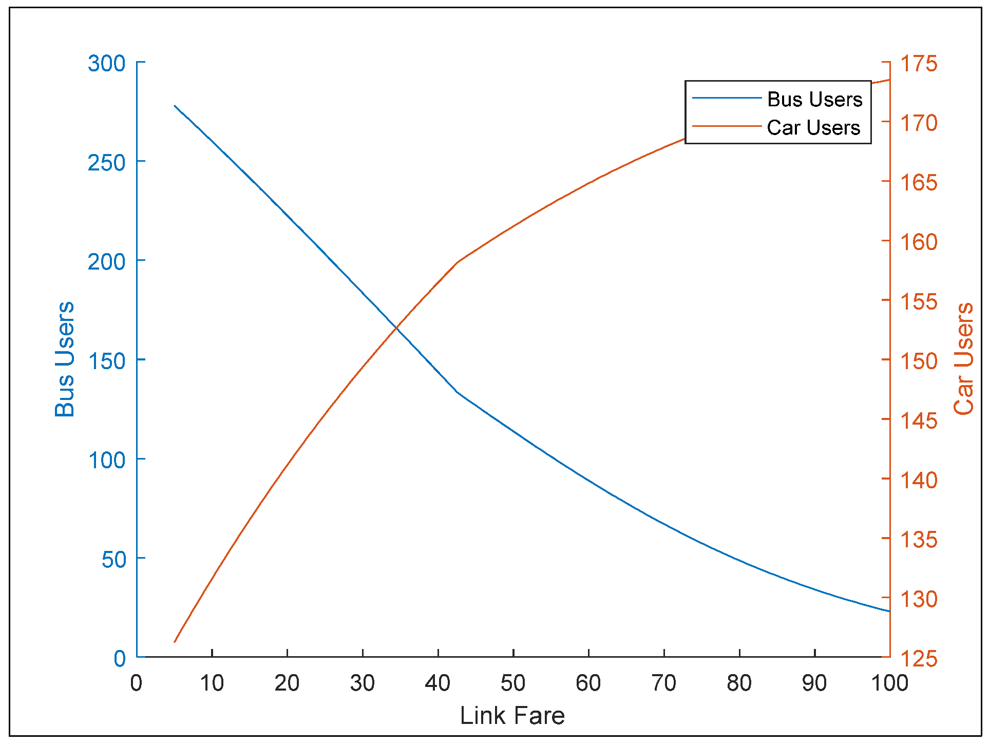
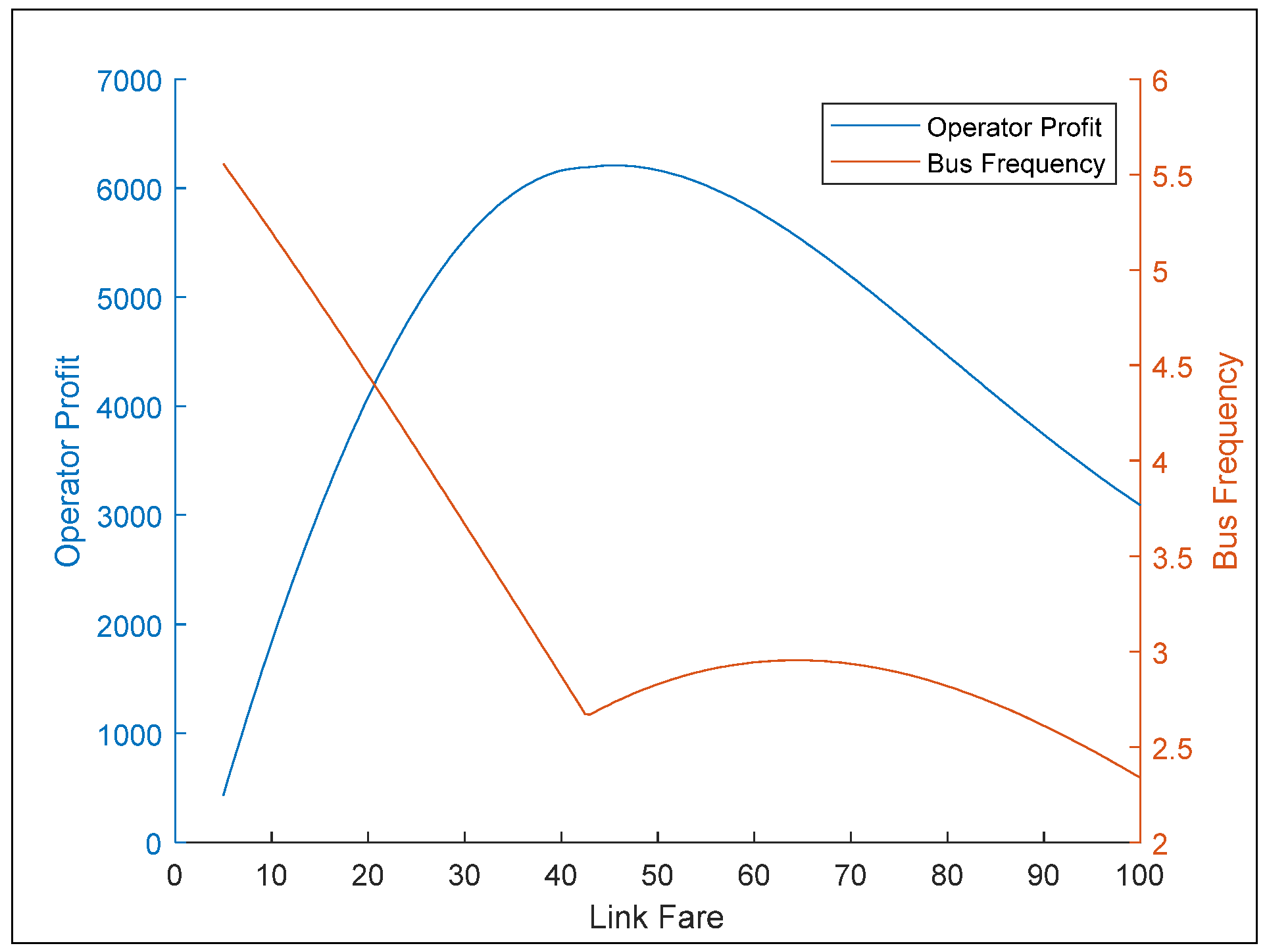
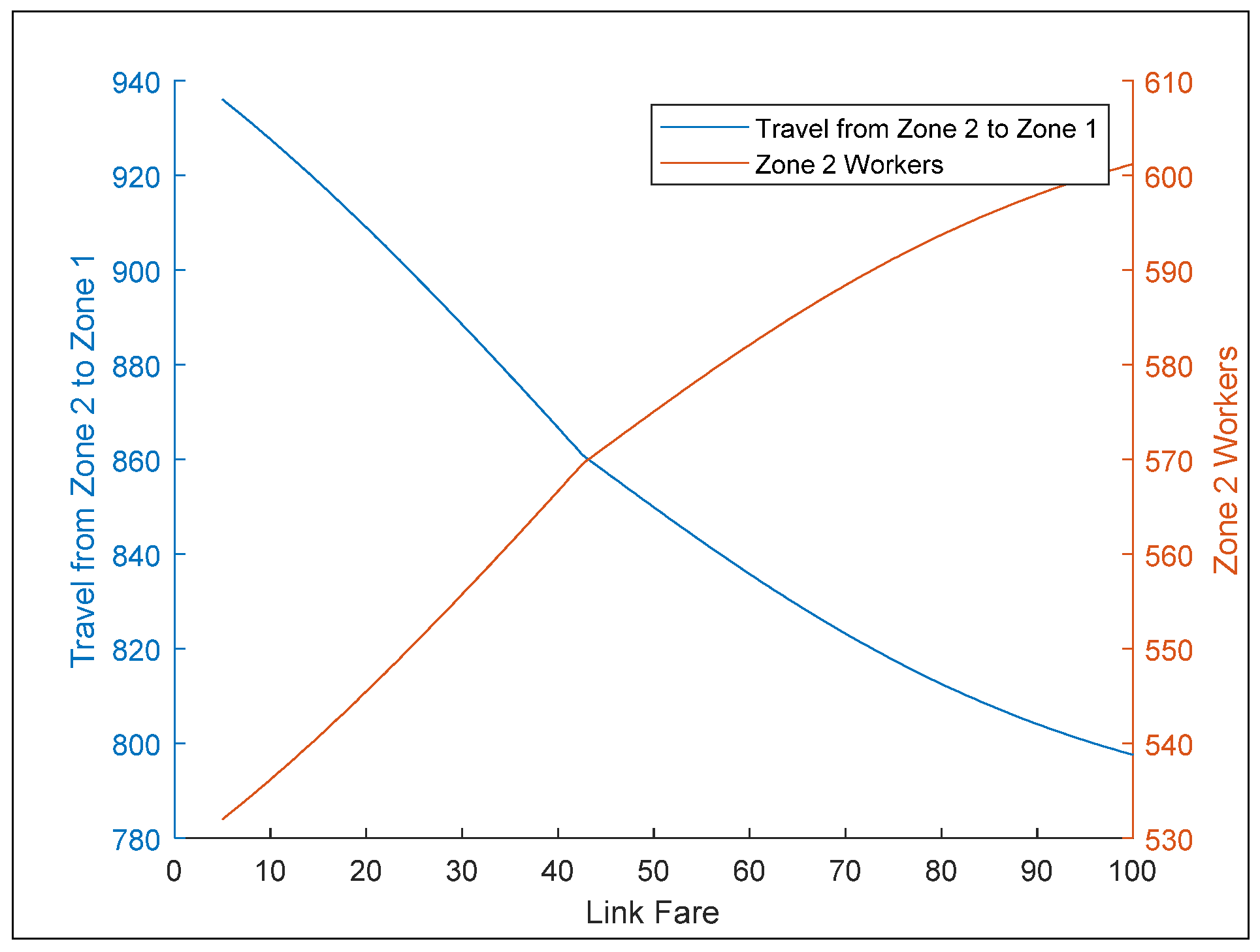
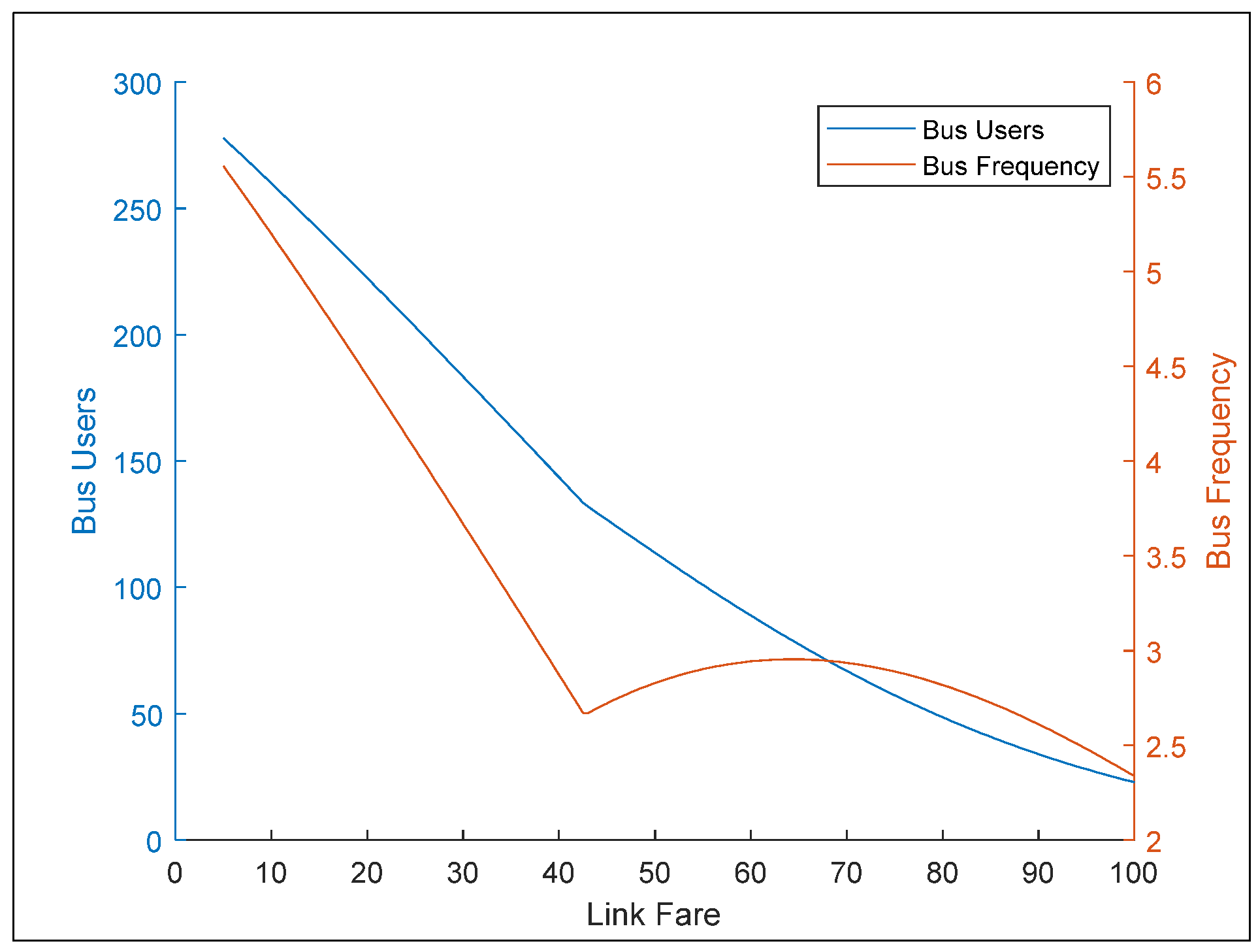
3.2. Simulations with Fare Range

In Figure 3, the solution algorithm of the unified equilibrium problem is shown. The residence choice behavior depends upon the selection of the work choice place (Figure 1). However, the choice of mode and route depends upon the generalized travel cost of private care and public bus as demonstrated in Equations (4)–(8). The generalized cost can be determined by using Equation (6). However, the cost of travel by public bus depends upon the number of vehicles (frequency) on the route, which is dependent upon waiting time. In Figure 4, the difference in the ridership between private car and public bus is observed against link fare. The link fare is one of the most important factors which impact the choice of mode [16]. Jin et al. [19] also confirms that the optimal fare structure exist above the minimum fare which is required to run a public transport structure. The change in modal shift is observed against link fare from 5 to 100 currencies. As it can be seen, when the bus fare is minimal, a greater number of users tend to use public transport for commuting. As the bus fare increases, there is a modal shift from public bus towards private car. When the link fare is further increased, the ridership of public bus is decreased while it is proportional to private car use. These simulated results are exactly in alignment with our assumption/objective of the study to find out if decreasing bus fare has a positive impact on public bus ridership and negative impact on private car use. These results also confirm that commuters always try to use the mode choice which minimizes traveling cost. In other words, it can be inferred that there is strong influence of link fare on the mode choice behavior of the commuters, who prefer to use the mode choice which minimizes traveling cost. The relationship of link fare, private car users, and public bus users is shown in Figure 4.
The relationship between link fare, bus users, and bus frequency are formulated in Figure 5. The change in bus frequency and bus users was observed against a range of link fare from 5 to 100 currencies. The bus frequency is formulated endogenously for achieving the strategic targets of attracting more commuters towards public bus while maximizing the profit of the bus operator. This bus frequency calculated from the bus operator model is incorporated into the unified equilibrium model to determine the costs of travel using specific mode (public bus or private car) on specific route. The user’s profit is calculated in terms of their traveling costs (measured in monetary units) between Zone 2 and 1. It can be seen from Figure 5 that increasing link fare increases the travel cost, which results in a decrease of public bus users. However, on the other hand, when link fare is lower, a greater number of commuters tend to use public bus because of lower traveling costs while using public bus; therefore, the bus frequency is more to accommodate the demand of traveling. In this situation where the link fare is small, the frequency is mostly determined by the constraint Equation (25). In other words, the bus company operates only the minimum number of buses necessary for its capacity. Figure 5 shows that when the link fare is 42.5 currencies, the bus frequency is 2.671, which shows that—for the range of fare between 30 to 55—the bus operator tries to operate at a lower frequency than in the case where a higher or lower fare is set. However, when the link fare is 65, then the bus frequency is locally maximum to accommodate the corresponding demand of traveling from Zone 2 to Zone 1. These findings also confirm similar results reported by [19]. However, if the link fare is further increased, the bus frequency keeps on decreasing which confirms that there is less demand of traveling between Zone 2 to Zone 1. In other words, the use of public bus would be further decreased if bus fare is increased. These results indicated that if the fares for bus services are not set appropriately, the service frequency may become extremely low, deteriorating the service quality of public transport.
The relationship between the profit of the public transport operator, link fare, and bus frequency are very interesting. When the link fare is very low, the bus frequency is more to accommodate the demand of the travelers. As can be seen from Figure 6, when the link fare is 5 (currency), the corresponding bus frequency is 5.557. In other words, lower fares attract more commuters; thus, bus frequency is higher to accommodate that demand. However, the service operator profit is less which may make the service operations unsustainable. When the link fare is 42.5, the bus frequency is 2.671, yet the service operator profit is 6189 (currencies). The operator profit is maximal at a fare rate of 45.5, making it 6208 (currencies) with a corresponding bus frequency of 2.734 vehicles. It is very interesting to note that when the operator profit is maximum, the bus frequency is not maximum. In other words, maximum profit does not mean maximum demand because frequency is determined based on demand in the network. Therefore, finding a good combination of operator profit and optimum frequency is important for sustainable operations of public bus. Additionally, it should be noted that demand varies with respect to travel cost which has link fare as one of the most important components. Therefore, determining a range of fares is also important for the feasibility of the transportation system in the network. As previous studies also suggested that users tend to use public transport if travel costs are lower, and level of service (bus frequency) is greater [33]. Further increasing the link fare from 45.5 (currencies) results in decrease in the operator profit, which ultimately leads to a decrease in bus frequency because of lower demand for transportation (Figure 6). This distinctive relationship might be explained in such a way that much lower or much higher fare makes the operations of the bus service unsustainable because of exceeding operations and traveling costs, respectively. Therefore, finding the correct combination of fares which optimizes the service operator profit, accommodates the demand for traveling between transportation network, and adjusts the service frequency as per demand is imperative for sustainable operations of the service. With the exact estimation of parameters, this model has the ability to optimize the overall performance of the transportation network. Therefore, the model proposed in this paper may be useful to search for more appropriate fare conditions while also dealing with land use markets.
Figure 7 shows the relationship between link fare, travel demand from Zone 2 to Zone 1 and workers in Zone 2. It is interesting to note that when the link fare increases, the travel demand between Zone 2 to Zone 1 decreases. In other words, it can be said that increase in link fare compels many of the residents to opt not to travel between Zones. In a similar pattern, increase in link fare urges the residents to seek work in Zone 2 to avoid traveling costs. Therefore, it can be seen that the number of Zone 2 residents increases as link fare increases. Contrary to that, the travel demand from Zone 2 to Zone 1 decreases with increase of link fare. These results are in agreement with the fact that travelers choose not to travel if traveling costs are higher between different zones. Again, the results confirm that this unified transport model has the ability to explain the strong relationship between land-use choices and transport systems.

4. Conclusions and Future Work

In this research study, we propose a unified model as a bi-level optimization problem. In the upper level, the fare of the bus operator is optimized which is constrained with bus frequency. In the lower level, the travel costs of commuters are minimized as a sub-assignment traffic model. The simulations are carried out for fixed fare (30 currencies) and a range of link fare (bus fare) to determine the trade-offs in which the benefits of the users as well as the public transport company are attained in such a way that users do not need to incur higher costs for traveling, as well as the bus operators’ operating costs are not exceeding their revenues. A simulation of the proposed model for a simple transit network was done to determine a win-win solution for both users and bus operator company. It is inferred from the simulation results that an optimal combination of fare and level of service (bus frequency) is required to maintain a good trade-off between the benefits of the users and service operators. The results imply that if there is an increase in link fare, the number of bus users will decrease, and more users will intend to use private cars. Previous research studies [18,19,20] also inferred similar findings which suggested that low fares increase the demand of users while high fares affect the mode and route choice behavior of the users. It is reported by Lam and Zhou [20] that users’ behavior can be influenced by adopting different fare policies, which leads to a change in link flows. Conversely, if link fare is decreased, more people adopt to use the public bus for traveling. The bus frequency is evaluated endogenously to accommodate the needs of the users (traveling demand) and it has been determined that it is not necessarily that maximum frequency guarantee the maximum profit of the service operator. However, it has been confirmed that at optimal link fare, a greater number of users would like to use public transport instead of private car. These findings are in agreement with the inferences made by Jin et al. [19]. It suggests that a reasonable fare is required to be set which maximizes the bus frequency which implies that a greater number of users are attracted towards the public bus. The results of the simple network case give a clear understanding that it is very necessary to adjust the link fare to attract more users and making a sustainable trade-off between conflicting objectives of users and service operator company. An increase in fare structure above or below a critical fare point can suddenly and significantly result in the drop of demand and service quality (frequency) [19]. An optimal fare is necessary for the determination of operators’ benefit and optimal service frequency [20]. The applications of this model to a real-world example can yield competing results for exact determination of link fare and bus frequency (LOS) when stakeholders have conflicting objectives in the transportation system. Moreover, the impacts of the link fare on land-use changes are also observed. It has been determined that an increase in travel costs impacts the land-use choices among the residents. The results also infer that there is a strong relationship between workplace, residence place, firms’, and landlords’ behavior with respect to the traveling costs.
The main contributions of this study can be summarized in these four conclusions: (a) land-use and transport systems are studied with combined modeling of route and mode choice along with residence choice behaviors; (b) the profit of the bus operator is optimized in a bi-level problem with minimization of users’ cost as a sub-assignment traffic model; (c) the equilibrium of travel behavior of users both with car and bus are analyzed to reveal their mode choices and relevant profit of operator at system equilibrium; (d) the dynamic interactions between users, bus operator, firms, workplace, and residence choices are studied to output the numerical analysis results at equilibrium under the influence of link fare. The academic contribution of this study is confirmed with the fact that land-use behavior is modeled along with the transport system (service operator and user behavior). As most of the studies do not explicitly model the behavior of land-use with the stakeholders in the transport system such as service operator and users. This study can be extended in the future for a larger network to study different variants of the model to better comprehend the nature of the model and its applications in the transportation system. However, it is pertinent to mention that extending this model to a larger transportation network would be a challenging task due to the high computational cost. Besides, different aims of system optimization can be set to obtain more realistic scenarios and different policies in the transport system can be analyzed. It would better help in explaining the mechanisms of how employing a policy can influence the transportation system dynamics in the next step.

Author Contributions

Conceptualization, N.A. and S.N.; Methodology, N.A.; Software, N.A. and H.Y.; Validation, N.A., S.N. and H.Y.; Formal analysis, N.A. and H.Y.; Investigation, N.A.; Resources, S.N.; Data curation, N.A.; Writing—original draft preparation, N.A.; Writing—review and editing, H.Y.; Visualization, N.A.; Supervision, S.N.; Project administration, N.A.; Funding acquisition, S.N. All authors have read and agreed to the published version of the manuscript.

Funding

JSPS KAKENHI grant number 21H01451.

Institutional Review Board Statement

Not applicable.

Informed Consent Statement

Not applicable.

Data Availability Statement

Not applicable.

Acknowledgments

This research work is part of the research fund, JSPS KAKENHI, grant number 21H01451.

Conflicts of Interest

The authors declare no conflict of interest.

References

  1. Xiao, L.-L.; Liu, T.-L.; Huang, H.-J. On the morning commute problem with carpooling behavior under parking space constraint. Transp. Res. Part B Methodol. 2016, 91, 383–407. [Google Scholar] [CrossRef]
  2. Guarda, P.; Galilea, P.; Paget-Seekins, L.; Ortúzar, J.D.D. What is behind fare evasion in urban bus systems? An econometric approach. Transp. Res. Part A Policy Pract. 2016, 84, 55–71. [Google Scholar] [CrossRef]
  3. Macioszek, E.; Kurek, A. The Use of a Park and Ride System—A Case Study Based on the City of Cracow (Poland). Energies 2020, 13, 3473. [Google Scholar] [CrossRef]
  4. Kitthamkesorn, S.; Chen, A.; Opasanon, S.; Jaita, S. A P-Hub Location Problem for Determining Park-and-Ride Facility Locations with the Weibit-Based Choice Model. Sustainability 2021, 13, 7928. [Google Scholar] [CrossRef]
  5. Macioszek, E.; Kurek, A. The Analysis of the Factors Determining the Choice of Park and Ride Facility Using a Multinomial Logit Model. Energies 2021, 14, 203. [Google Scholar] [CrossRef]
  6. LeBlanc, L.J. Transit system network design. Transp. Res. Part B Methodol. 1988, 22, 383–390. [Google Scholar] [CrossRef]
  7. Tirachini, A. Estimation of travel time and the benefits of upgrading the fare payment technology in urban bus services. Transp. Res. Part C Emerg. Technol. 2013, 30, 239–256. [Google Scholar] [CrossRef]
  8. Yang, Y.; Deng, L.; Wang, Q.; Zhou, W. Zone Fare System Design in a Rail Transit Line. J. Adv. Transp. 2020, 2020, 2470579. [Google Scholar] [CrossRef]
  9. Tom, V.M.; Mohan, S. Transit Route Network Design Using Frequency Coded Genetic Algorithm. J. Transp. Eng. 2003, 129, 186–195. [Google Scholar] [CrossRef]
  10. Canca, D.; De-Los-Santos, A.; Laporte, G.; Mesa, J.A. Integrated Railway Rapid Transit Network Design and Line Planning problem with maximum profit. Transp. Res. Part E Logist. Transp. Rev. 2019, 127, 1–30. [Google Scholar] [CrossRef]
  11. Uchida, K.; Sumalee, A.; Watling, D.; Connors, R. Study on optimal frequency design problem for multimodal network using probit-based user equilibrium assignment. Transp. Res. Rec. 2002, 236–245. [Google Scholar] [CrossRef]
  12. Constantin, I.; Florian, M. Optimizing frequencies in a transit network: A nonlinear bi-level programming approach. Int. Trans. Oper. Res. 1995, 2, 149–164. [Google Scholar] [CrossRef]
  13. Zhu, W.; Chen, M.; Wang, D.; Ma, D. Policy-Combination Oriented Optimization for Public Transportation Based on the Game Theory. Math. Probl. Eng. 2018, 2018, 7510279. [Google Scholar] [CrossRef]
  14. Yu, B.; Yang, Z.; Yao, J. Genetic Algorithm for Bus Frequency Optimization. J. Transp. Eng. 2010, 136, 576–583. [Google Scholar] [CrossRef]
  15. Zhou, J.; Lam, W.H.; Heydecker, B.G. The generalized Nash equilibrium model for oligopolistic transit market with elastic demand. Transp. Res. Part B Methodol. 2005, 39, 519–544. [Google Scholar] [CrossRef]
  16. Harris, A.E.; Thomas, R.; Boyle, D. Metropolitan Atlanta Rapid Transit Authority Fare Elasticity Model. Transp. Res. Rec. J. Transp. Res. Board 1999, 1669, 123–128. [Google Scholar] [CrossRef]
  17. Cummings, C.P.; Fairhurst, M.; Labelle, S.; Stuart, D. Market Segmentation of Transit Fare Elasticities. Transp. Q. 1989, 43, 407–420. [Google Scholar]
  18. Wang, Q.; Schonfeld, P.; Deng, L. Profit Maximization Model with Fare Structures and Subsidy Constraints for Urban Rail Transit. J. Adv. Transp. 2021, 2021, 6659384. [Google Scholar] [CrossRef]
  19. Jin, Z.; Schmöcker, J.-D.; Maadi, S. On the interaction between public transport demand, service quality and fare for social welfare optimisation. Res. Transp. Econ. 2019, 76, 100732. [Google Scholar] [CrossRef]
  20. Lam, W.H.K.; Zhou, J. Optimal Fare Structure for Transit Networks with Elastic Demand. Transp. Res. Rec. J. Transp. Res. Board 2000, 1733, 8–14. [Google Scholar] [CrossRef]
  21. Spasovic, L.N.; Schonfeld, P.M. Method for optimizing transit service coverage. Transp. Res. Rec. 1993, 1402, 28–39. [Google Scholar]
  22. Wirasinghe, S. Nearly optimal parameters for a rail/feeder-bus system on a rectangular grid. Transp. Res. Part A Gen. 1980, 14, 33–40. [Google Scholar] [CrossRef]
  23. Chang, S.K.; Schonfeld, P.M. Optimal Dimensions of Bus Service Zones. J. Transp. Eng. 1993, 119, 567–585. [Google Scholar] [CrossRef]
  24. Byrne, B.F. Cost minimizing positions, lengths and headways for parallel public transit lines having different speeds. Transp. Res. 1976, 10, 209–214. [Google Scholar] [CrossRef]
  25. Holroyd, E.M. The Optimum Bus Service: A Theoretical Model for a Large Uniform Urban Area. 1967. Available online: https://trid.trb.org/view/693339 (accessed on 30 October 2021).
  26. Byrne, B.F. Public transportation line positions and headways for minimum user and system cost in a radial case. Transp. Res. 1975, 9, 97–102. [Google Scholar] [CrossRef]
  27. Hurdle, V.F. Minimum Cost Locations for Parallel Public Transit Lines. Transp. Sci. 1973, 7, 340–350. [Google Scholar] [CrossRef]
  28. Kocur, G.; Hendrickson, C. Design of Local Bus Service with Demand Equilibration. Transp. Sci. 1982, 16, 149–170. [Google Scholar] [CrossRef]
  29. Kuah, G.K.; Perl, J. Optimization of Feeder Bus Routes and Bus-Stop Spacing. J. Transp. Eng. 1988, 114, 341–354. [Google Scholar] [CrossRef]
  30. Chang, S.K.; Schonfeld, P.M. Multiple period optimization of bus transit systems. Transp. Res. Part B Methodol. 1991, 25, 453–478. [Google Scholar] [CrossRef]
  31. Spasovic, L.; Boile, M.; Bladikas, A. Bus transit service coverage for maximum profit and social welfare. Transp. Res. Board. 1994, 1451, 12–22. [Google Scholar]
  32. Li, Z.-C.; Lam, W.H.K.; Wong, S.C. The Optimal Transit Fare Structure under Different Market Regimes with Uncertainty in the Network. Networks Spat. Econ. 2009, 9, 191–216. [Google Scholar] [CrossRef]
  33. Chien, S.I.-J.Y.; Tsai, C.F.M. Optimization of Fare Structure and Service Frequency for Maximum Profitability of Transit Systems. Transp. Plan. Technol. 2007, 30, 477–500. [Google Scholar] [CrossRef]
  34. Van Nes, R. Multilevel Network Optimization for Public Transport Networks. Transp. Res. Board. 2002, 2, 50–57. [Google Scholar] [CrossRef]
Figure 1. Worker’s choice structure.
Sustainability 14 00139 g001
Figure 2. A simple transit network.
Sustainability 14 00139 g002
Figure 3. The algorithm for solving the unified equilibrium. The asterisk “*” shows the estimated value of v.
Sustainability 14 00139 g003
Figure 4. Relationship between link fare, bus users, and car users.
Sustainability 14 00139 g004
Figure 5. Relationship between link fare, bus users, and bus frequency.
Sustainability 14 00139 g005
Figure 6. Relationship between link fare, operator profit, and bus frequency.
Sustainability 14 00139 g006
Figure 7. Relationship between link fare and land-use change.
Sustainability 14 00139 g007
Table 1. Pertinent Models for the Design of Transit Network.
AuthorsObjective FunctionTransit ModeDecision VariablesPassenger Demand
Spasovic and Schonfled (1993) [21]Min. of operator and user costBusRoute length, headway, spacing, stop spacingUniform and linear
Wirasinghe and Seneviratne (1986) [22]Min. of operator and user costRailRoute lengthGeneral, inelastic
Chang and Schonfeld (1993) [23]Min. of operator and user costBusRoute spacing, zone length, headwayUniform, inelastic
Byrne (1976) [24]Min. of operator and user costBus and railRoute spacing, headway, and lengthsUniform, inelastic
Holroyd (1976) [25] Min. of operator and user costBusRoute spacingUniform, inelastic
Byrne and Vuchic (1972) [26]Min. of operator and user costBusRoute spacing and headwayUniform, inelastic
Hurdle (1973) [27]Min. of operator and user costBusRoute density and frequencyGeneral linear, inelastic
Kocur and Hendrickson (1982) [28]Max. operator profit, Max. user profit, etc. BusRoute spacing, fare and headwayUniform elastic
Kuah and Perl (1988) [29]Min. of operator and user costFeeder bus to railRoute spacing, stop spacing, and headwayGeneral inelastic
Chang and Schonfeld (1989) [30]Max. operator profit, Min. user profit, etc.BusRoute spacing, fare and headwayIrregular elastic
Spasovic et al. (1994) [31]Max. operator profit, Max. social welfareBusRoute length, route spacing, fare and headwayUniform elastic
Li et al., (2009) [32]Max. operator profit, Min. user profit, etc.Bus and railRoute length, fareUniform elastic
Chien and Tsai (2007) [33]Max. operator profit, Min. user profit, etc.RailRoute length, fare, and headwayUniform elastic
Rob Van Nes (2002) [34]Max. operator profit, Max. social welfareBus and carRoute length, route spacing, Uniform and linear
Wang et al. (2021) [18]Max. operator profit, Max. social welfareBusRoute length, headway, and fare Uniform elastic
Table 2. Settings of Parameters.
(a) General parameters
ParameterValue
Total Population_N1000
Logit   parameter _ θ 1 0.04
Logit   parameter _ θ 2 0.03
Logit   parameter _ θ 3 0.02
Logit   parameter _ κ 0.05
Logit   parameter _ μ 0.2
Firm   space _ γ 20
Firm   labor _ λ 10
(b) Zone parameters
Zone Code
i
Zone Size
D i
Zone Production
V i
110002000
220000
( c )   Path   settings ,   δ i j k , a
Path NoResidenceFirmCar LinkBus Link
11100
22110
32101
42200
(d) Link parameters
Link Code
a
Link Free Flow Time
t 0 , a
Capacity
C a
BPR Alpha
α a
BPR Beta
β a
1201000.53
2205000
Table 3. Model output results for fixed fare.
Passenger FlowResidence Choice Behavior
Zone 1 flow, f11111.489 Zone   1   residential   rent ,   r 1 0
Zone 2 to 1 car flow, f21c149.352 Zone   1   business   rent ,   r 1 10.378
Zone 2 to 1 bus flow, f21p183.414 Zone   2   residential   rent ,   r 2 −79.736
Zone 2 flow, f22555.745 Zone   2   business   rent ,   r 2 −78.617
Land Use Choice BehaviorZone 1 households5020
Zone   1   residential   area ,   l 1 111Zone 2 households14,980
Zone   1   business   area ,   l 1 889Workplace Choice Behavior
Zone   2   residential   area ,   l 2 888 Zone   1   wage ,   w 1 22.458
Zone   2   business   area ,   l 2 1112 Zone   2   wage ,   w 2 0
Mode Choice Behavior Zone   1   employees ,   y 1 8880
Car   travel   cos t ,   c 21 c 63.314 Zone   2   employees ,   y 2 11,120
Bus   travel   cos t ,   c 21 p 58.178Firm Choice Behavior
Car   use   probability ,   p / 21 c 0.449 Zone   1   firms ,   m 1 444
Bus   use   probability ,   p / 21 p 0.551 Zone   2   firms ,   m 2 556
Bus Operator Model
Optimum   frequency ,   v k 3.668 Operator   profit ,   ξ ( v k ) 4035.1
Publisher’s Note: MDPI stays neutral with regard to jurisdictional claims in published maps and institutional affiliations.

