
Improving Energy Efficiency in Buildings Using an Interactive Mathematical Programming Approach


Abstract
1. Introduction
2. Materials and Methods
2.1. Overview
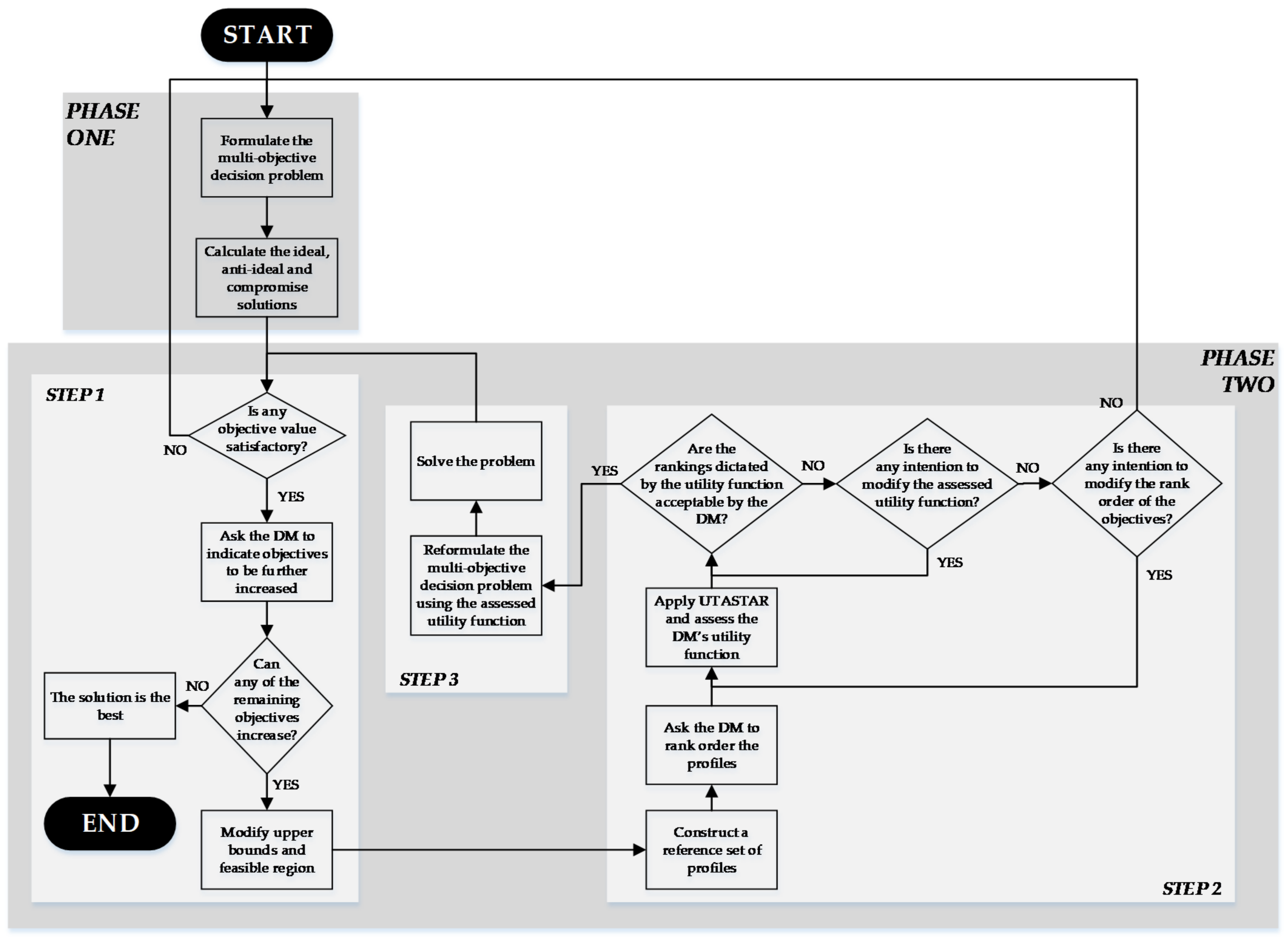
- In the first phase, each individual objective of (1) is first minimized and then maximized over the set of the feasible solutions, thus providing lower and upper bounds for the objectives. Given that are minimized in (1), the lower bounds represent the ideal values of the objectives, and remain the same throughout the whole process, while the upper bounds represent the anti-ideal ones, and are refined during the second phase of the procedure. In addition, an initial efficient solution, i.e., a solution, which is not dominated by any other acceptable solution in the decision space is estimated that is closest to the ideal one with respect to the weighted Tchebycheff norm [15].
- In the second phase, an iterative process is followed, which comprises three successive steps. The first step can be viewed as a learning process of the trade-offs among the objectives for the DM. Through questions and answers, this step refines the upper bounds, thus gradually reducing the feasible region of the decision problem. The second step can be viewed as a learning process of the DM’s preferences. During this step, the DM is asked to rank, according to his/her preferences, a reference set of fictitious non-dominated decision profiles. This subjective ranking is then used by a UTASTAR model to generate the DM’s utility function u, over the intervals created by the lower and upper limits of the objectives’ values, and use them in transforming the decision problem (1) in the following:where, is the vector of the values of the objectives of the initial Problem (1). The decision Problem (2) is solved in the third step of the process, the solution is presented to the DM, and the iterations restart until a solution is reached that will be sufficiently satisfactory for the DM, so that he/she will not wish to further improve it.
2.2. The Interactive Mathematical Programming Approach
2.2.1. Phase One
2.2.2. Phase Two
- The upper bound values are equal to the solutions of the corresponding problems (4), obtained in phase one;
- The optimal values of the objectives are equal to the values obtained via the solution of the multi-objective Problem (5) in phase one.
Step 1
- : the subset of G, which comprises the objectives that the DM insists to decrease;
- : the complement of in G.
Step 2
Step 3
3. Application Example
3.1. Overview of the Decision Problem
- the addition or not, in the building’s walls, ceiling, and floor, of an insulation layer of maximum permissible thickness 0.10 m and material chosen among the alternatives of Table 6;
- the space cooling system among the alternatives of Table 8;
- the addition or not of a solar collector system among the alternatives of Table 11.
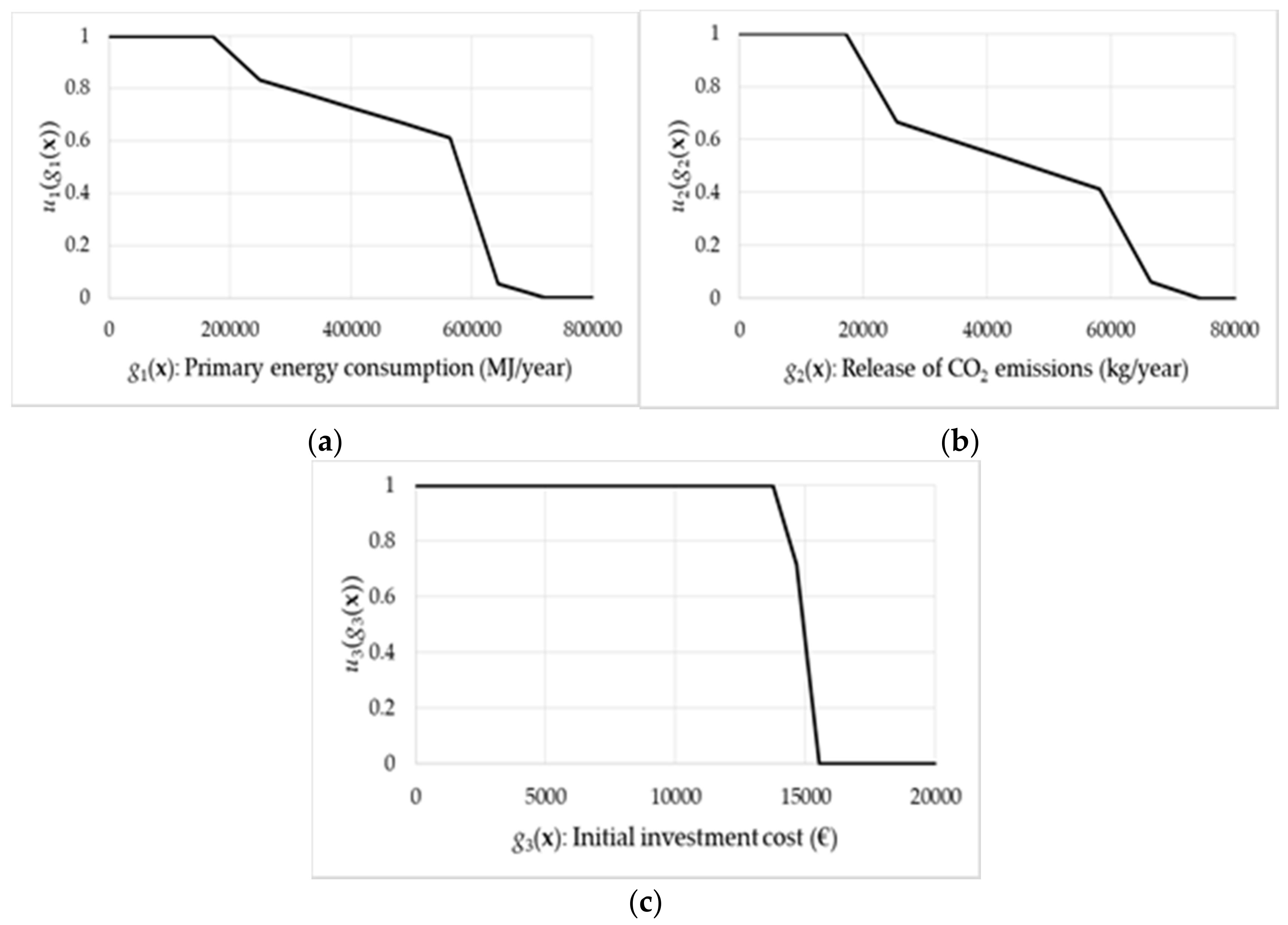
- The primary energy consumption ;
- the release of CO2 emissions ; and
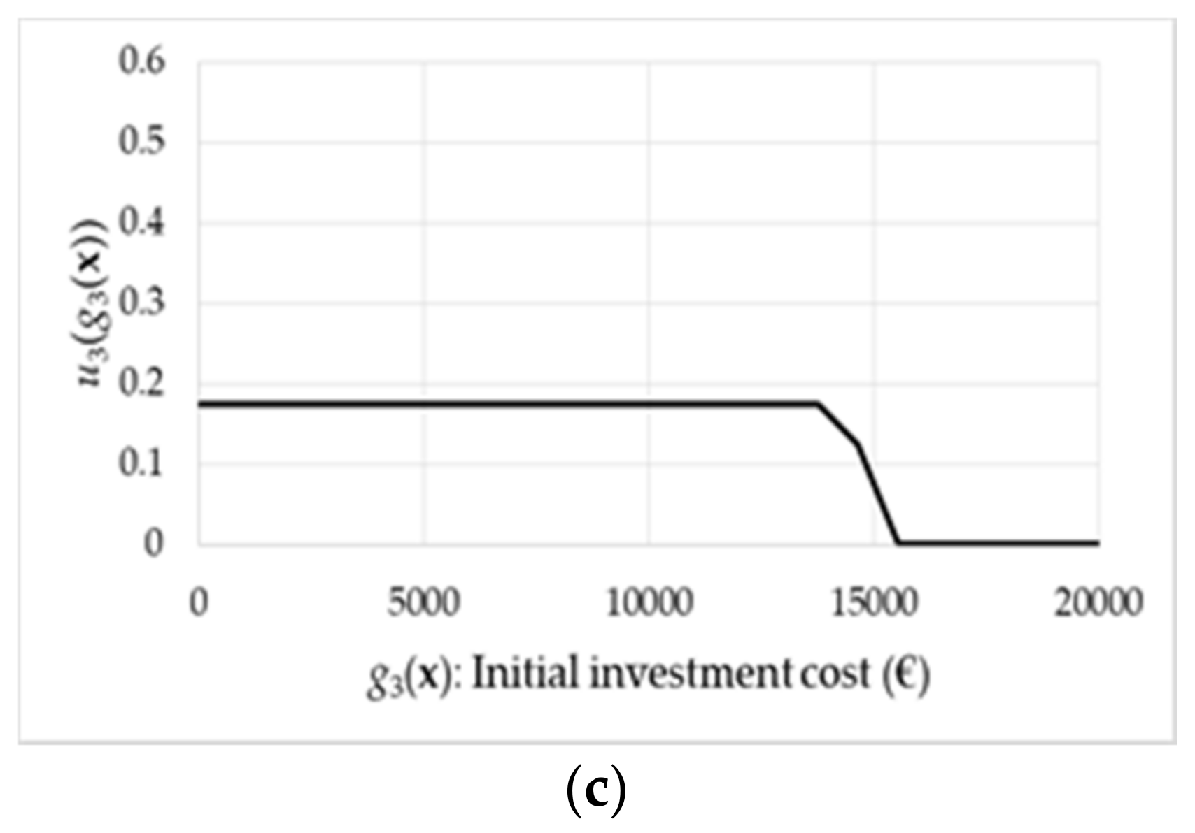
- the initial investment cost .
3.2. Application of the Interactive Mathematical Programming Approach
3.2.1. Phase One
3.2.2. Phase Two-Iteration 1-Step 1
- ;
- ;
- ;
3.2.3. Phase Two-Iteration 1-Step 2
3.2.4. Phase Two-Iteration 1-Step 3
3.2.5. Phase Two-Iteration 2-Step 1
4. Discussion
5. Conclusions
Author Contributions
Funding
Institutional Review Board Statement
Informed Consent Statement
Data Availability Statement
Conflicts of Interest
Appendix A. The UTASTAR Method
- The global value of all reference actions , , is first expressed in terms of the marginal values , and then in terms of the variables , according to (A8), through the following relationships:
- For each pair of actions, which are consecutive in the given ranking, error terms are introduced using the following relationship:
- The following linear programming problem is solved:
- The existence of multiple or near optimal solutions of the Problem (A11) is examined (stability analysis), and the mean additive value function of those (near) optimal solutions is found, which maximize the objective functions:on the polyhedron of the constraints of the Problem (A11), bounded by the following additional constraint:where is the optimal value of Problem (A11) and is a very small positive number.
Appendix B. The Multi-Objective Decision Model of the Application Example
Appendix B.1. Parameters and Decision Variables

| Parameters | Description |
|---|---|
| DR | Number of building’s doors; here |
| dr | Index to DR; |
| Area of door dr (m2); here | |
| Temperature correction factor of construction part dr; here | |
| V | Number of available door types |
| v | Index to V; |
| Thermal transmittance of door type (W/m2 K) | |
| Cost of door type v (€/m2) |
| Parameters | Description |
|---|---|
| WN | Number of building’s windows; here |
| wn | Index to WN; |
| Area of window wn (m2); here | |
| Temperature correction factor of construction part wn; here | |
| Frame factor of window wn (%); here | |
| Correction factor for shading of window wn (%); here | |
| Correction factor for movable devices of window wn (%); here | |
| S | Number of available window types |
| s | Index to S; |
| Number of available sub-types of window type s | |
| t | Index to ; |
| Effective total solar energy transmittance of window sub-type t (%) | |
| Thermal transmittance of window sub-type t (W/m2K) | |
| Cost of window sub-type (€/m2) |
| Parameters | Description |
|---|---|
| WL | Number of walls; here |
| wl | Index to WL; |
| Area of wall wl (m2); here and | |
| Temperature correction factor of construction part wl; here | |
| W | Number of available wall structures |
| w | Index to W; |
| Number of known layers of structure w, regarding material and thickness | |
| kwl | Index to ; |
| Thickness of known layer kwl of wall structure w (m) | |
| Thermal conductivity of material of known layer kwl of wall structure w (W/mK) | |
| Cost of material of known layer kwl of wall structure w (€/m3) | |
| Number of unknown layers of structure w; here (insulation layer) | |
| y | Index to ; |
| Maximum permissible thickness of layer y of structure w (m); here | |
| Number of available materials for layer y of structure w | |
| c | Index to ; |
| Thermal conductivity of material c of unknown layer y of structure w (W/mK) | |
| Cost of material c of unknown layer y of structure w (€/m3) |
| Parameters | Description |
|---|---|
| CE | Number of ceilings; here |
| ce | Index to CE; |
| Area of ceiling ce (m2); here | |
| Temperature correction factor of construction part ce; here | |
| D | Number of available ceiling structures |
| d | Index to D; |
| Number of known layers of structure d, regarding material and thickness | |
| kcl | Index to ; |
| Thickness of known layer kcl of structure d (m) | |
| Thermal conductivity of material of known layer kcl of structure d (W/mK) | |
| Cost of material of known layer kcl of structure d (€/m3) | |
| Number of unknown layers of structure d; here (insulation layer) | |
| f | Index to ; |
| Maximum permissible thickness of layer f of structure d (m); here | |
| Number of available materials for layer f of structure d | |
| a | Index to ; |
| Thermal conductivity of material a of unknown layer f of structure d (W/mK) | |
| Cost of material a of unknown layer f of structure d (€/m3) |
| Parameters | Description |
|---|---|
| FL | Number of floors; here |
| fl | Index to FL; |
| Area of floor fl (m2); here | |
| Temperature correction factor of construction part fl; here | |
| H | Number of available floor structures |
| h | Index to H; |
| Number of known layers of structure h, regarding material and thickness | |
| kfl | Index to ; |
| Thickness of known layer kfl of structure h (m) | |
| Thermal conductivity of material of known layer kfl of structure h (W/mK) | |
| Cost of material of known layer kfl of structure h (€/m3) | |
| Number of unknown layers of structure h; here (insulation layer) | |
| e | Index to ; |
| Maximum permissible thickness of layer e of structure h (m); here | |
| Number of available materials for layer e of structure h | |
| g | Index to ; |
| Thermal conductivity of material g of unknown layer e of structure h (W/mK) | |
| Cost of material g of unknown layer e of structure h (€/m3) |
| Parameters | Description |
|---|---|
| EHI | Number of available electrical heating systems’ categories |
| ehi | Index to EHI; |
| Number of available systems of category ehi | |
| ehj | Index to ; |
| Generation efficiency of system ehj of category ehi (%) | |
| Installation cost of system ehj of category ehi (€) | |
| NEHI | Number of available non-electrical heating systems’ categories |
| nehi | Index to NEHI; |
| Number of available systems of category nehi | |
| nehj | Index to ; |
| Generation efficiency of system nehj of category nehi (%) | |
| Installation cost of system nehj of category nehi (€) | |
| Parameter; equals 1, if system nehj of category nehi uses fuel fuel, else equals 0 |
| Parameters | Description |
|---|---|
| ECI | Number of available electrical cooling systems categories |
| eci | Index to ECI; |
| Number of available systems of category eci | |
| ecj | Index to ; |
| Generation efficiency of system ecj of category eci (%) | |
| Installation cost of system ecj of category eci (€) |
| Parameters | Description |
|---|---|
| EWI | Number of available electrical DHW systems’ categories |
| ewi | Index to EWI; |
| Number of available systems of category ewi | |
| ewj | Index to ; |
| Generation efficiency of system ewj of category ewi (%) | |
| Installation cost of system ewj of category ewi (€) | |
| NEWI | Number of available non-electrical DHW systems’ categories |
| newi | Index to NEWI; |
| Number of available systems of category newi | |
| newj | Index to ; |
| Generation efficiency of system newj of category newi (%) | |
| Installation cost of system newj of category newi (€) | |
| Parameter; equals 1, if system newj of category newi uses fuel fuel, else equals 0 |
| Parameters | Description |
|---|---|
| EHCI | Number of available combined electrical heating-cooling systems’ categories |
| ehci | Index to EhCI; |
| Number of available systems of category ejci | |
| ehcj | Index to ; |
| Generation efficiency of system ehcj of category ehci (%) | |
| Installation cost of system ecj of category eci (€) |
| Parameters | Description |
|---|---|
| EHWI | Number of available combined electrical heating-DHW systems’ categories |
| ehwi | Index to EHWI; |
| Number of available systems of category ehwi | |
| ehwj | Index to ; |
| Generation efficiency of system ehwj of category ehwi (%) | |
| Installation cost of system ehwj of category ehwi (€) | |
| NEHWI | Number of available non-electrical combined heating-DHW systems’ categories |
| nehwi | Index to NEHWI; |
| Number of available systems of category nehwi | |
| nehwj | Index to ; |
| Generation efficiency of system nehwj of category nehwi (%) | |
| Installation cost of system nehwj of category nehwi (€) | |
| Parameter; equals 1, if system nehwj of category nehwi uses fuel fuel, else equals 0 |
| Parameters | Description |
|---|---|
| Area of solar collector (m2); here | |
| Correction factor for shading of solar collector (%); here | |
| U | Number of available solar collectors systems’ categories |
| u | Index to U; |
| Number of available solar collectors systems of category u | |
| b | Index to ; |
| Generation efficiency of system b of category u (%) | |
| Installation cost of system b of category u (€/m2) |
| Parameters | Description |
|---|---|
| FUEL | Number of fuels available for heating and DHW; here |
| fuel | Index to FUEL; ; here is oil and is gas |
| Conversion factor of fuel fuel to CO2 emissions (kg of CO2/kg of fuel); here and | |
| Conversion factor of fuel fuel to energy (MJ/kg of fuel); here and | |
| Emissions factor of electricity producing station (kg of CO2/MJ); here | |
| Return rate of electricity producing stations; here |
| Parameters | Description |
|---|---|
| n | Month index; ; 1 corresponds to January, 2 to February, etc. |
| Duration of month n (s) | |
| Average external temperature at building’s location in month n (°C) | |
| Solar radiation on window wn in month n (MJ/m2/month) | |
| Solar radiation on solar collector in month n (MJ/m2/month) | |
| Air density at building’s location (kg/m3) | |
| Air heat at building’s location (J/kg°C) | |
| Air volume (m3) |
| Parameters | Description |
|---|---|
| Internal design temperature during heating season (°C); here | |
| Internal design temperature during cooling season (°C); here | |
| Parameter; equals 1, if heating is required for month n, else equals 0; here and | |
| Parameter; equals 1, if cooling is required for month n, else equals 0; here and | |
| Parameter; equals 1, if hot water supply is required for month n, else equals 0; here | |
| Average monthly heat gains (W); here 1 | |
| Average energy requirements for hot water use (MJ/month); here 1 |
| Variable | Description |
|---|---|
| Doors choice; equals 1, if type v is selected, else equals 0 | |
| Windows choice; equals 1, if subtype t of type s is selected, else equals 0 | |
| Wall structure choice; equals 1, if structure w is selected, else equals 0 | |
| Wall material choice; equals 1, if material c is selected for layer y of wall structure w, else equals 0 | |
| Thickness of material added in layer y of wall structure w (m) | |
| Ceiling structure choice; equals 1, if structure d is selected, else equals 0 | |
| Ceiling material choice; equals 1, if material a is selected for layer f of ceiling structure d, else equals 0 | |
| Thickness of material added in layer f of ceiling structure d (m) | |
| Floor structure choice; equals 1, if structure h is selected, else equals 0 | |
| Floor material choice; equals 1, if material g is selected for layer e of floor structure h, else equals 0 | |
| Thickness of material added in layer e of floor structure h (m) | |
| Electrical heating system choice; equals 1, if system ehj of category ehi is selected, else equals 0 | |
| Non-electrical heating system choice; equals 1, if system nehj of category nehi is selected, else equals 0 | |
| Electrical cooling system choice; equals 1, if system ecj of category eci is selected, else equals 0 | |
| Electrical DHW system choice; equals 1, if system ewj of category ewi is selected, else equals 0 | |
| Non-electrical DHW system choice; equals 1, if system newj of category newi is selected, else equals 0 | |
| Electrical heating–cooling system choice; equals 1, if system ehcj of category ehci is selected, else equals 0 | |
| Electrical heating–DHW system choice; equals 1, if system ehwj of category ehwi is selected, else equals 0 | |
| Non-electrical heating–DHW system choice; equals 1, if system nehwj of category nehwi is selected, else equals 0 | |
| Solar collector choice; equals 1 if system b of category u is selected, else equals 0 | |
| x | Vector of all decision variables x |
Appendix B.2. Multi-Objective Decision Model
References
- Costa-Carrapiço, I.; Raslan, R.; González, J.N. A systematic review of genetic algorithm-based multi-objective optimisation for building retrofitting strategies towards energy efficiency. Energy Build. 2020, 210, 109690. [Google Scholar] [CrossRef]
- Hashempour, N.; Taherkhani, R.; Mahdikhani, M. Energy performance optimization of existing buildings: A literature review. Sustain. Cities Soc. 2020, 54, 101967. [Google Scholar] [CrossRef]
- Wulfinghoff, D.R. Energy Efficiency Manual; Energy Institute Press: Wheaton, MD, USA, 1999. [Google Scholar]
- Diakaki, C.; Grigoroudis, E.; Kolokotsa, D. Towards a multi-objective optimization approach for improving energy efficiency in buildings. Energy Build. 2008, 40, 1747–1754. [Google Scholar] [CrossRef]
- Diakaki, C.; Grigoroudis, E.; Kabelis, N.; Kolokotsa, D.; Kalaitzakis, K.; Stavrakakis, G. A multi-objective decision model for the improvement of energy efficiency in buildings. Energy 2010, 35, 5483–5496. [Google Scholar] [CrossRef]
- Diakaki, C.; Grigoroudis, E. Applying genetic algorithms to optimise energy efficiency in buildings. In Multicriteria Decision Aid and Artificial Intelligence: Links, Theory and Applications; Doumpos, M., Grigoroudis, E., Eds.; John Wiley & Sons Ltd: Hoboken, NJ, USA, 2013; pp. 309–333. [Google Scholar] [CrossRef]
- Diakaki, C.; Grigoroudis, E.; Kolokotsa, D. Performance study of a multi-objective mathematical programming modelling approach for energy decision-making in buildings. Energy 2013, 59, 534–542. [Google Scholar] [CrossRef]
- Ren, H.; Zhou, W.; Gao, W.; Wu, Q. A mixed-integer linear optimization model for local energy system planning based on simplex and branch-and-bound algorithms. In Life System Modeling and Intelligent Computing; Li, K., Fei, M., Jia, L., Irwin, G.W., Eds.; Springer: Berlin/Heidelberg, Germany, 2010; Volume 6328, pp. 361–371. [Google Scholar] [CrossRef]
- Asadi, E.; Da Silva, M.G.; Antunes, C.H.; Dias, L. Multi-objective optimization for building retrofit strategies: A model and an application. Energy Build. 2012, 44, 81–87. [Google Scholar] [CrossRef]
- Üçtug, F.G.; Yukseltan, E. A linear programming approach to household energy conservation: Efficient allocation of budget. Energy Build. 2013, 49, 200–208. [Google Scholar] [CrossRef]
- Karmellos, M.; Kiprakis, A.; Mavrotas, G. A multi-objective approach for optimal prioritization of energy efficiency measures in buildings: Model, software and case studies. Appl. Energy 2015, 139, 131–150. [Google Scholar] [CrossRef]
- Bayata, O.; Temiz, I. Developing a model and software for energy efficiency optimization in the building design process: A case study in Turkey. Turk. J. Electr. Eng. Comput. Sci. 2017, 25, 4172–4186. [Google Scholar] [CrossRef]
- Shakouri, G.H.; Rahmani, M.; Hosseinzadeh, M.; Kazemi, A. Multi-objective optimization-simulation model to improve the buildings’ design specification in different climate zones of Iran. Sustain. Cities Soc. 2018, 40, 394–415. [Google Scholar] [CrossRef]
- Nielsen, A.N.; Jensen, R.L.; Larsen, T.S.; Nissen, S.B. Early stage decision support for sustainable building renovation—A review. Build. Environ. 2016, 103, 165–181. [Google Scholar] [CrossRef]
- Siskos, J.; Despotis, D.K. A DSS oriented method for multiobjective linear programming problems. Decis. Support. Syst. 1989, 5, 47–55. [Google Scholar] [CrossRef]
- Siskos, Y.; Yannacopoulos, D. UTASTAR: An ordinal regression method for building additive value functions. Investig. Oper. 1985, 5, 39–53. [Google Scholar]
- Kreider, J.F.; Curtiss, P.; Rabl, A. Heating and Cooling for Buildings, Design for Efficiency; McGraw-Hill: New York, NY, USA, 2002. [Google Scholar]
- Zopounidis, C.; Despotis, D.K.; Kamaratou, I. Portfolio selection using the ADELAIS multiobjective linear programming System. Comput. Econ. 1998, 11, 189–204. [Google Scholar] [CrossRef]
- Lee, S.H.; Hong, T.; Piette, M.A.; Taylor-Lange, S.C. Energy retrofit analysis toolkits for commercial buildings: A review. Energy 2015, 89, 1087–1100. [Google Scholar] [CrossRef]


| Type | Thermal Transmittance (W/m2 °C) | Cost (€/m2) |
|---|---|---|
| 1. Hollow-core flush door | 2.7 | 800 |
| 2. Solid-core flush door with single glazing (17% glass) | 2.1 | 1000 |
| Type | Subtype | Thermal Transmittance (W/m2 °C) | Effective Total Solar Energy Transmittance (%) | Cost (€/m2) |
|---|---|---|---|---|
| 1. Single glazing | 1. Typical glazing | 5.0 | 80 | 40 |
| 2. Double glazing | 1. 4-20-4, uncoated, air filled | 2.6 | 72 | 55 |
| 2. 4-12-4, coated, argon filled | 1.6 | 76 | 65 |
| Structure | Layer | Material | Thickness (m) | Thermal Conductivity (W/m °C) | Cost (€/m3) |
|---|---|---|---|---|---|
| 1 | 1 | Plaster | 0.025 | 0.87 | 10 |
| 2 | Brick (complex) | 0.150 | 0.72 | 23 | |
| 3 | Plaster | 0.025 | 0.87 | 10 | |
| 2 | 1 | Plaster | 0.025 | 0.87 | 10 |
| 2 | Brick (complex) | 0.060 | 0.72 | 6.2 | |
| 3 | Brick (complex) | 0.060 | 0.72 | 6.2 | |
| 4 | Plaster | 0.025 | 0.87 | 10 |
| Structure | Layer | Material | Thickness (m) | Thermal Conductivity (W/m °C) | Cost (€/m3) |
|---|---|---|---|---|---|
| 1 | 1 | Tiles | 0.02 | 1.00 | 55 |
| 2 | Concrete | 0.15 | 0.72 | 55 | |
| 2 | 1 | Tiles | 0.02 | 1.00 | 55 |
| 2 | Wood | 0.03 | 0.17 | 70 |
| Structure | Layer | Material | Thickness (m) | Thermal Conductivity (W/m °C) | Cost (€/m3) |
|---|---|---|---|---|---|
| 1 | 1 | Tiles | 0.01 | 1.00 | 55 |
| 2 | Concrete | 0.15 | 0.72 | 55 | |
| 2 | 1 | Wood | 0.02 | 0.17 | 85 |
| 2 | Concrete | 0.15 | 0.72 | 55 |
| Material | Thermal Conductivity (W/m °C) | Cost (€/m3) |
|---|---|---|
| 1. Polystyrene | 0.036 | 200 |
| 2. Mineral fiber | 0.042 | 180 |
| 3. Plastic fiber | 0.020 | 300 |
| Category | Type | Generation Efficiency (%) | Cost (€) |
|---|---|---|---|
| Electrical systems | |||
| 1. Resistance-based | 1. Dry core storage boiler type 1 | 100 | 5000 |
| 2. Dry core storage boiler type 2 | 85 | 4200 | |
| Non-electrical systems | |||
| 1. Oil-based | 1. Condensing | 83 | 5300 |
| 2. Standard oil boiler | 62 | 4700 | |
| 2. Natural-gas based | 1. Condensing | 85 | 5800 |
| 2. Floor mounted boiler | 55 | 4500 |
| Category | Type | Generation Efficiency (%) | Cost (€) |
|---|---|---|---|
| 1. Water cooled electric | 1. <12,000 BTU | 200 | 500 |
| 2. <18,000 BTU | 230 | 800 | |
| 3. <24,000 BTU | 250 | 1200 |
| Category | Type | Generation Efficiency (%) | Cost (€) |
|---|---|---|---|
| Electrical systems | |||
| 1. Resistance-based | 1. Electric CPSU | 100 | 7200 |
| 2. Water storage boiler | 85 | 5800 | |
| Non-electrical systems | |||
| 1. Oil-based | 1. Condensing combi | 81 | 6200 |
| 2. Combi | 70 | 5800 | |
| 2. Natural-gas based | 1. Condensing combi | 84 | 7200 |
| 2. Combi | 65 | 5700 |
| Category | Type | Generation Efficiency (%) | Cost (€) |
|---|---|---|---|
| Electrical systems | |||
| 1. Resistance-based | 1. Electric immersion | 100 | 1200 |
| 2. Electric instantaneous at point of use | 85 | 1000 | |
| Non-electrical systems | |||
| 1. Oil-based | 1. Oil boiler/circulator | 80 | 1000 |
| 2. Oil single burner | 60 | 800 | |
| 2. Natural-gas based | 1. Circulator built into a gas warm air system type 1 | 73 | 850 |
| 2. Circulator built into a gas warm air system type 2 | 60 | 650 |
| Category | Type | Generation Efficiency (%) | Cost (€) |
|---|---|---|---|
| 1. Flat collector | 1. Type 1 | 90 | 900 |
| 2. Type 2 | 80 | 600 | |
| 2. Vacuum hear pipe CPC collector | 1. Type 1 | 72 | 780 |
| 2. Type 2 | 67 | 500 |
| Decisions and Criteria | Type of Solution | ||||||
|---|---|---|---|---|---|---|---|
| Minimize | Maximize | Compromise | |||||
| Door type | 2 | 2 | 1 | 1 | 1 | 2 | 1 |
| Window type/subtype | 2/2 | 2/2 | 1/1 | 1/1 | 1/1 | 2/2 | 2/2 |
| Wall structure | 1 | 1 | 2 | 2 | 2 | 1 | 2 |
| Wall insulation thickness (m) | 0.10 | 0.10 | 0.00 | 0.00 | 0.00 | 0.10 | 0.07 |
| Wall insulation material | 3 | 3 | - | - | - | 3 | 3 |
| Ceiling structure | 1 | 1 | 2 | 2 | 2 | 1 | 2 |
| Ceiling insulation thickness (m) | 0.10 | 0.10 | 0.00 | 0.00 | 0.00 | 0.10 | 0.07 |
| Ceiling insulation material | 3 | 3 | - | - | - | 3 | 3 |
| Floor structure | 2 | 2 | 1 | 1 | 1 | 2 | 1 |
| Floor insulation thickness (m) | 0.10 | 0.10 | 0.00 | 0.00 | 0.00 | 0.10 | 0.07 |
| Floor insulation material | 3 | 3 | - | - | - | 3 | 3 |
| Heating system type | EHC | NEH | EHC | EHW | EHW | EHW | EHC |
| Heating system category/type | 1/3 | 2/1 | 1/1 | 1/2 | 1/2 | 1/1 | 1/3 |
| Cooling system type | - | EC | - | EC | EC | EC | - |
| Cooling system category/type | - | 1/3 | - | 1/1 | 1/1 | 1/3 | - |
| Hot water supply system type | NEW | NEW | NEW | - | - | - | NEW |
| Hot water supply system category/type | 1/1 | 2/1 | 2/2 | - | 1/2 | - | 2/2 |
| Solar collector category/type | 1/1 | 1/1 | - | - | - | 1/1 | 2/2 |
| : Primary energy consumption (MJ/year) | 13,593 | 13,970 | 321,276 | 722,123 | 722,123 | 32,475 | 19,582 |
| : Release of CO2 emissions (kg CO2/year) | 1400 | 810 | 32,758 | 74,559 | 74,559 | 3353 | 1986 |
| : Initial investment cost (€) | 21,987 | 27,637 | 7524 | 12,674 | 12,674 | 28,187 | 15,540 |
| Information | Primary Energy Consumption (MJ/Year) i = 1 | Release of CO2 Emissions (kg CO2/Year i = 2 | Initial Investment Cost (€) i = 3 |
|---|---|---|---|
| Ideal solution (lower bound) | 13,593 | 810 | 7524 |
| Initial compromise solution | 19,582 | 1986 | 15,540 |
| Anti-ideal solution | 722,123 | 74,559 | 28,187 |
| Initial upper bound | 722,123 | 74,559 | 28,187 |
| Rate of closeness to the ideal solution | 0.85% | 1.59% | 38.80% |
| Profile | Primary Energy Consumption (MJ/Year) | Release of CO2 Emissions (kg CO2/Year) | Initial Investment Cost (€) | DM’s Ranking |
|---|---|---|---|---|
| 13,593 | 810 | 15,540 | 3 | |
| 92,319 | 9004 | 14,650 | 2 | |
| 171,044 | 17,199 | 13,759 | 1 | |
| 249,770 | 25,393 | 12,868 | 4 | |
| 328,495 | 33,587 | 11,978 | 5 | |
| 407,221 | 41,782 | 11,087 | 6 | |
| 485,947 | 49,976 | 10,196 | 7 | |
| 564,672 | 58,171 | 9306 | 8 | |
| 643,398 | 66,365 | 8415 | 9 | |
| 722,123 | 74,559 | 7524 | 10 |
| Information | Primary Energy Consumption (MJ/Year) i = 1 | Release of CO2 Emissions (kg CO2/Year) i = 2 | Initial Investment Cost (€) i = 3 |
|---|---|---|---|
| Ideal solution (lower limit) | 13,593 | 810 | 7524 |
| New compromise solution | 166,640 | 17,199 | 11,147 |
| Anti-ideal solution | 722,123 | 74,559 | 28187 |
| New upper bound | 722,123 | 74,559 | 15,540 |
| Rate of closeness to the ideal solution | 21.60% | 22.22% | 17.53% |
| Decisions and Criteria | Initial Compromise Solution | Final Compromise Solution |
|---|---|---|
| Door type | 1 | 1 |
| Window type/subtype | 2/2 | 2/1 |
| Wall structure | 2 | 1 |
| Wall insulation thickness (m) | 0.07 | 0 |
| Wall insulation material | 3 | - |
| Ceiling structure | 2 | 2 |
| Ceiling insulation thickness (m) | 0.07 | 0.01 |
| Ceiling insulation material | 3 | 1 |
| Floor structure | 1 | 1 |
| Floor insulation thickness (m) | 0.07 | 0.07 |
| Floor insulation material | 3 | 1 |
| Heating system type | EHC | EHC |
| Heating system category/type | 1/3 | 1/1 |
| Cooling system type | - | - |
| Cooling system category/type | - | - |
| Hot water supply system type | NEW | NEW |
| Hot water supply system category/type | 2/2 | 2/2 |
| Solar collector category/type | 2/2 | 1/1 |
| : Primary energy consumption (MJ/year) | 19,582 | 166,640 |
| : Release of CO2 emissions (kg CO2/year) | 1986 | 17,199 |
| : Initial investment cost (€) | 15,540 | 11,147 |
Publisher’s Note: MDPI stays neutral with regard to jurisdictional claims in published maps and institutional affiliations. |
© 2021 by the authors. Licensee MDPI, Basel, Switzerland. This article is an open access article distributed under the terms and conditions of the Creative Commons Attribution (CC BY) license (https://creativecommons.org/licenses/by/4.0/).
Share and Cite
Diakaki, C.; Grigoroudis, E. Improving Energy Efficiency in Buildings Using an Interactive Mathematical Programming Approach. Sustainability 2021, 13, 4436. https://doi.org/10.3390/su13084436
Diakaki C, Grigoroudis E. Improving Energy Efficiency in Buildings Using an Interactive Mathematical Programming Approach. Sustainability. 2021; 13(8):4436. https://doi.org/10.3390/su13084436
Chicago/Turabian StyleDiakaki, Christina, and Evangelos Grigoroudis. 2021. "Improving Energy Efficiency in Buildings Using an Interactive Mathematical Programming Approach" Sustainability 13, no. 8: 4436. https://doi.org/10.3390/su13084436
APA StyleDiakaki, C., & Grigoroudis, E. (2021). Improving Energy Efficiency in Buildings Using an Interactive Mathematical Programming Approach. Sustainability, 13(8), 4436. https://doi.org/10.3390/su13084436